| Issue |
A&A
Volume 700, August 2025
|
|
|---|---|---|
| Article Number | L2 | |
| Number of page(s) | 8 | |
| Section | Letters to the Editor | |
| DOI | https://doi.org/10.1051/0004-6361/202555557 | |
| Published online | 25 July 2025 | |
Letter to the Editor
A gravitational acceleration model to explain the double-peaked narrow emission lines shifted in the same direction
School of Physical Science and Technology, Guangxi University, No. 100, Daxue East Road, Nanning 530004, PR China
⋆ Corresponding author: This email address is being protected from spambots. You need JavaScript enabled to view it.
Received:
17
May
2025
Accepted:
5
July
2025
Abstract
In this Letter, we propose a new, oversimplified, but potentially effective gravitational acceleration model to interpret the double-peaked narrow emission lines (DPNELs) shifted in the same direction. We adopted the framework of a merging kpc-scale dual-core system in an elliptical orbit, which includes an emission-line galaxy (ELG) with clear narrow line regions (NLRs) merging with a companion galaxy that clearly lacks emission line features. Due to gravitational forces induced by both galaxies on the NLRs, the accelerations of the far-side and near-side NLR components may share the same vector direction when projected along the line of sight (LoS), leading the velocities of the observed DPNELs to shift in the same direction. Our simulations indicate that the probability of producing double-peaked features shifted in the same direction reaches 5.81% in merging kiloparsec-scale (kpc-scale) dual-core systems containing ELGs. In addition to the expected results from our proposed model, we also identified a unique galaxy, SDSS J001050.52−103246.6, whose apparent DPNELs, shifted in the same direction, could plausibly be explained by the gravitational acceleration model. This proposed model provides a new path to explain DPNELs shifted in the same direction in a scenario where the two galaxies would align along LoS in kpc-scale dual-core systems.
Key words: galaxies: active / galaxies: individual: SDSS J0010–1032 / galaxies: nuclei / quasars: emission lines
© The Authors 2025
 Open Access article, published by EDP Sciences, under the terms of the Creative Commons Attribution License (https://creativecommons.org/licenses/by/4.0), which permits unrestricted use, distribution, and reproduction in any medium, provided the original work is properly cited.
This article is published in open access under the Subscribe to Open model. This email address is being protected from spambots. You need JavaScript enabled to view it. to support open access publication.
1. Introduction
Double-peaked narrow emission lines (DPNELs) have been investigated since the 1980s, especially in active galactic nuclei (AGNs), as discussed in Heckman et al. (1981, 1984), Keel (1985), and Veilleux (1991). These features in the spectra are commonly attributed to two kinematically distinct emission components with different velocities, as discussed in Gerke et al. (2007), Wang et al. (2009), and Liu et al. (2010). Since DPNEL galaxies play a critical role in studying the dynamics of AGN narrow line regions (NLRs) and merging galaxies, they have motivated the establishment of large and homogeneous samples to investigate their properties through statistical analyses given their unclear physical origins (Smith et al. 2010; Ge et al. 2012; Wang & Zhou 2012; Müller-Sánchez et al. 2015; Comerford et al. 2018; Wang et al. 2019; Zheng et al. 2025).
At the current stage, the physical origins of DPNELs can be categorized into three primary scenarios. Firstly, DPNELs can arise from biconical geometry and disturbed gas kinematics in the NLR, driven by AGN radiation pressure, as discussed in Fischer et al. (2011), Shen et al. (2011), Fu et al. (2012), and Barrows et al. (2013). Secondly, rotating disk-like NLR structures in AGNs can produce DPNELs due to the orbital motion of ionized gas, as proposed in Müller-Sánchez et al. (2011), Kharb et al. (2015), and Maschmann et al. (2023). Thirdly, DPNELs can stem from the orbital motion of kiloparsec-scale (kpc-scale) dual-core systems containing independent NLRs, as discussed in Zhou et al. (2004), Xu & Komossa (2009), and Fu et al. (2011).
In conventional DPNELs, the two emission components arising from either NLRs kinematics or dual-core systems exhibit similar shifted emission line features, one of the peaks is redshifted and the other peak is blueshifted relative to the redshift of the host galaxy. However, a peculiar subclass of DPNELs displays both emission components shifted in the same direction, a phenomenon unexplained by existing scenarios. We propose a gravitational acceleration model to elucidate its physical origin for the first time. However, this subclass of DPNELs may arise from inaccurate determinations of the host galaxy redshift, indicating the need for reliable redshift measurements.
In Section 2, we present our main hypotheses of the gravitational acceleration model. In Section 3, we perform our main simulations and offer a discussion on SDSS J001050.52−103246.6, whose DPNELs are shifted in the same direction. Our summary and conclusion are presented in Section 4. Throughout this Letter, we adopt the cosmological parameters H0 = 70 km s−1 Mpc−1, ΩM = 0.3, and ΩΛ = 0.7.
2. Main hypothesis
2.1. Gravitational acceleration model
The first proposed gravitational acceleration model is based on a kpc-scale dual-core system, where the two galaxies orbit each other in an elliptical trajectory at kpc-scale separations. The emission-line galaxy (ELG) containing the far-side and near-side NLR components is designated as the main galaxy, while the orbiting non-ELG is designated as the companion galaxy. We assume that the two galaxies are initially located at the apocenter of the elliptical orbit and are aligned along the line of sight (LoS). Adopting the ionized cone model of NLRs from Liu et al. (2013), we assume the NLRs are symmetric mass distributions positioned on opposite sides of the main galaxy. Figure 1 illustrates the model configuration.
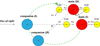 |
Fig. 1. Diagram of the gravitational acceleration model with the two galaxies initially located at the apocenter of the elliptical orbit. The circles filled in red and blue represent the main and companion galaxies, respectively. The circles filled in yellow represent the NLRs of the main galaxy. The black arrows represent the gravitational force vectors. The green dashed line represents the clockwise elliptical orbit, with θ marking the rotation angle. System I indicates the initial positions of the galaxies in the simulation, aligned along LoS, while system II indicates their final positions. The arrow in the left region marks LoS. |
Based on the law of universal gravitation and Newton’s laws of motion, the near-side (NLR1) and far-side (NLR2) of NLRs, under the gravitational forces of both main and companion galaxies, yield individual accelerations, which can be described as:
 (1)
(1)
where Mc and Mm are the total stellar masses of the main and companion galaxies; dc1, dc2, dm1, and dm2 denote the distances from the companion/main galaxy to NLR1/NLR2. The gravitational forces between NLRs are not considered in the acceleration computations, nor is there any consideration of the gas mass of the companion galaxy in estimating its total mass. Detailed discussions can be found in Appendices A.1 and A.2. Here, the leftward direction is defined as positive. Both accelerations can thus attain positive values (indicating the same vector direction) with different magnitudes after projecting along LoS. Consequently, a period of acceleration (hereafter acceleration duration) causes both NLRs to obtain velocities shifted in the same direction. The acceleration process always requires that the distances between NLRs and galaxies exceed 0.05 kpc.
2.2. Simulation parameters
To determine the parameters required for performing simulations based on the gravitational acceleration model, we adopted the following methods to derive reasonable parameters.
We utilize the Structured Query Language (SQL) search tool provided by Sloan Digital Sky Survey (SDSS) to collect galaxy samples for the main (main sample) and companion (companion sample) galaxies to determine their total stellar masses.
For the main sample, the emission line fluxes of Hα, Hβ, [O III]λ5007 Å, [N II]λ6584 Å, and [S II]λ6717, 6731 Å doublet, along with the corresponding uncertainties, were selected from the SDSS GalSpecLine database, while the total stellar masses (the parameter mstellar_median and corresponding uncertainty mstellar_err) were selected from the stellarMassPCAWiscM11 database. The selection criteria for the main-sample are provided in Appendix A.3, yielding 159 911 galaxies in the main sample.
For the companion sample, the selected parameters and the first three criteria are the same as those for the main sample. An additional requirement imposes flux < 3*flux_err for the same emission lines, ensuring negligible emission line features. This results in 8916 galaxies being collected in the companion sample. The distributions of the logarithmic total stellar masses of both samples are shown in the top-left region of panel a in Figure 2.
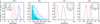 |
Fig. 2. Simulation results for the model adopting an elliptical orbit with an eccentricity of 0.2 and with galaxies initially at apocenter. Panel (a): Histograms filled in red and blue show the logarithmic total stellar mass distributions of the main and companion galaxies in the 10 000 satisfied simulations with DPNELs shifted in the same direction. Here, the top left inset displays the mass distributions for the galaxies in the collected main-sample (histogram in purple) and companion-sample (histogram in green). Panel (b): Histograms filled in red, blue, and cyan show the distributions of the smaller blueshifted velocity, larger blueshifted velocity, and velocity separation of DPNELs shifted in the same direction; the arrows in red, blue, and black mark the smaller blueshifted velocity, larger blueshifted velocity, and velocity separation of SDSS J001050.52−103246.6. Panel (c): Histograms in red and blue show the distributions of RNLRs and galaxy separation; the distribution of RNLRs/D is shown in the top right region. Panel (d): Histograms filled in red and blue show the distributions of the acceleration duration and orbital period; the distribution of the acceleration duration/orbital period (t/T) is shown in the top right region. All the histograms are normalized to the peak value. |
Given that the total stellar mass of the main galaxy can be determined from the main sample, the size of the NLRs (the distance between NLRs and central black hole, hereafter RNLRs) should also be reasonably determined. Therefore, we combine the known empirical RNLRs − L[O III] correlation in AGNs from Liu et al. (2013) (L[O III] as the [O III] 5007 Å luminosity) with the L[O III] − M∗ correlation derived from our main sample (M* as the logarithmic total stellar mass) to determine RNLRs via total stellar mass. The RNLRs − L[O III] correlation in the literature is expressed as
![Mathematical equation: $$ \begin{aligned} \log \left(\frac{R_{\rm NLRs}}{\mathrm{pc}}\right) = (0.25 \pm 0.02) \times \log \left(\frac{L_{[\mathrm{O}\,iii ]}}{10^{42}\,\mathrm{erg/s}}\right) + (3.75 \pm 0.03). \end{aligned} $$](/articles/aa/full_html/2025/08/aa55557-25/aa55557-25-eq2.gif) (2)
(2)
Using the collected main-sample, we can estimate the L[O III] − M∗ correlation:
![Mathematical equation: $$ \begin{aligned} \log \left(L_{[\mathrm{O}\,iii ]}/\mathrm{erg/s}\right) = \alpha \times M_{*} + \beta . \end{aligned} $$](/articles/aa/full_html/2025/08/aa55557-25/aa55557-25-eq3.gif) (3)
(3)
Using the least-trimmed-squares regression technique, the best-fit parameters were measured: α = 0.44 ± 0.01 and β = 35.52 ± 0.06 (the 1σ uncertainties are determined through this technique), with a rank correlation coefficient of 0.34. Figure 3 plots the best-fitting results. Although our main sample comprises ELGs (rather than AGNs), we retained this approach to minimize the number of free parameters in simulations. Therefore, with the help of the two correlations, an accepted dependence of RNLRs on the total stellar mass is established.
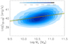 |
Fig. 3. Information on the correlation between L[O III] and logarithmic total stellar mass for the galaxies in the main sample. The green solid line indicates the best-fitting results and the red dashed lines indicate the corresponding 5σ confidence bands. Contour levels in different colors are related to number densities shown in color bar in the top region. |
The separation between the main and companion galaxies (hereafter, the galaxy separation) is assumed to be between three and ten times RNLRs, leading to a maximum value of ∼35 kpc. Detailed descriptions of the determination of galaxy separation are provided in Appendix A.4. To neglect the orbit decay, the acceleration duration is constrained to be less than 10% of the orbital period of the kpc-scale dual-core system, limiting the maximum rotation angle to θ < 36°. The orbital period of the elliptical orbital motion is calculated via Kepler’s third law:
 (4)
(4)
where r is the semi-major axis, measured as D/(1 + e); then, D is the galaxy separation and e is the eccentricity of the elliptical orbit; Mm and Mc are the total stellar masses of the main and companion galaxies, respectively; and T is the orbital period. Additionally, we imposed a minimum projected velocity separation of 100 km/s between DPNELs peaks to ensure resolvable double-peaked profiles. Detailed descriptions are provided in Appendix A.5.
Moreover, to possibly recreate the realistic galaxy merging process, we enforced two NLR displacement constraints to prevent mergers between galaxies and NLRs. The distance between the far-side NLR (NLR2) and the center of the main galaxy is at least 0.05 kpc (dm2 > 0.05 kpc), and the near-side NLR (NLR1) is confined to half the galaxy separation (dm1 < D/2).
3. Main results
3.1. Simulation results
Building on the hypotheses outlined in Section 2, we introduce the workflow and key parameters of our oversimplified simulations, based on the gravitational acceleration model, adopting an elliptical orbit with an eccentricity of 0.2 (as an example), and with the two galaxies initially located at the apocenter of the elliptical orbital path. In each simulation, the total stellar masses of the main and companion galaxies are randomly drawn from the main-sample and companion-sample, respectively. The RNLRs of the main galaxy is then calculated via the RNLRs − L[O III] and L[O III] − M∗ correlations (Section 2.2). The corresponding uncertainties of both correlations are also incorporated in the computational process. The effects of adopting the uncertainties on the simulation results are discussed in Appendix A.6. The galaxy separation is determined by multiplying RNLRs by a random factor between 3 and 10. The acceleration duration is randomly assigned between 0% and 10% of the orbital period, which was computed using Equation (4) with the selected total stellar masses and the semi-major axis determined by the galaxy separation. During the acceleration phase, the duration is divided into 50 time segments, with the shifted velocities and spatial extensions of the NLRs calculated in each segment. We retained the simulations where the velocity separation exceeds 100 km/s and NLR extensions satisfy the NLR displacement constraints.
Through 172 000 simulation trials, 10 000 runs satisfy our selection criteria, indicating that approximately 5.81% of kpc-scale dual-core systems with ELGs may exhibit DPNELs shifted in the same direction. Figure 2 presents the simulation results related to the galaxies with DPNELs shifted in the same direction. The logarithmic total stellar mass distributions of the main and companion galaxies differ significantly, with mean values of 10.35 and 11.69, respectively. The velocity separation has a mean value of 321 km/s, slightly higher than the mean velocity separation of common DPNELs of 300 km/s reported in Ge et al. (2012). The RNLRs span from 1.04 kpc to 3.12 kpc, while galaxy separations extend from 3.75 kpc to 22.07 kpc. The acceleration duration varies from 0.53 Myr to 22.53 Myr, while the orbital period is in the range of 22.43−462.12 Myr.
3.2. An instance with DPNELs shifted in the same direction
To identify galaxies exhibiting DPNELs shifted in the same direction as a case study, we searched SDSS DR16 and identified one object SDSS J001050.52−103246.6 (hereafter, SDSS J0010). We analyzed its spectroscopic data using methodologies similar to our prior work in Chen et al. (2025). The detailed spectroscopic handling procedure of SDSS J0010 is provided in Appendix B.
The spectroscopic results of SDSS J0100 are shown in Figure 4. Consequently, we obtained the velocity parameters of DPNELs of SDSS J0100, with blueshifted velocities of −343.32 ± 17.27 km/s and −41.51 ± 36.71 km/s, and a velocity separation of  km/s. These values are annotated in panel b of Figure 2 with colored arrows. However, as its blueshifted velocity offsets and velocity separation fully align with our simulated parameter space, its DPNELs shifted in the same direction can be interpreted by our model from a purely numerical simulation perspective. Detailed discussions of DPNELs shifted in the same direction of SDSS J0010 are provided in Appendix B. Furthermore, we are preparing a sample consisting of galaxies similar to SDSS J0010 with such peculiar DPNELs features.
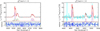 |
Fig. 4. Spectroscopic results of SDSS J001050.52−103246.6. Left and right panels present the best-fitting results to the emission lines around Hα and Hβ, respectively. In both panels, the cyan components indicate the spectrum after subtracting the host galaxy starlight; the thick red components indicate the best-fitting results; and the solid lines in the bottom region of each panel indicate residuals. In the left panel, the thin red and thin blue Gaussian components from left to right indicate the double-peaked features of narrow [N II]λ6550 Å, Hα, [N II]λ6585 Å, [S II]λ6718 Å, and [S II]λ6732 Å; the green Gaussian components indicate the extended emission components in [N II]λ6550 Å, Hα, and [N II]λ6585 Å. In the right panel, the thin red and thin blue Gaussian components from left to right indicate the double-peaked features of narrow Hβ, [O III]λ4959 Å, and [O III]λ5007 Å. In each panel, the corresponding χ2/d.o.f. related to the best-fitting results is marked in the title. |
3.3. Discussions of stated assumptions
Figure 1 depicts the projection-aligned scenario. In reality, an inclination exists between the galaxy pair and between the galaxies and NLRs. Considering that only gravity and velocity components perpendicular to LoS contribute to the final results, we assume the NLRs and galaxies are initially aligned along the line-of-sight. Additionally, the discussions of the model configuration reality are provided in Appendix A.7.
Galaxy mergers inherently involve orbital velocities. In our framework, the NLRs and the main galaxy share identical orbital velocities, resulting in equal contributions to the shifted velocities of the near-side and far-side NLRs. While this affects the magnitude of blueshifted velocities, but not the velocity separation, the orbital velocity was not included in the computational procedure.
Our model assumes an elliptical orbit for the merging galaxy pair. The simulation results presented in Figure 2 are simulated by the model in an elliptical orbit with an eccentricity of 0.2 and with galaxies initially at the apocenter. We also explore the effects of different eccentricities of the elliptical orbital path and the initial positions where the galaxies are located on the final simulation results. The detailed discussions are provided in Appendix C.
If both galaxies have emission line features, their mutual gravitational interactions in a kpc-scale dual-core system could theoretically produce four-peaked narrow emission lines. It will be an interesting challenge to detect the galaxies with four-peaked narrow emission lines in the future.
4. Conclusion
We propose a brand new gravitational acceleration model to explain a special subclass of DPNELs exhibiting velocities shifted in the same direction. Through an oversimplified simulation of 17 2000 trials, we found 10 000 cases meeting the criteria for generating such features, implying a 5.81% probability of arising DPNELs shifted in the same direction in merging kpc-scale dual-core systems containing ELGs. Meanwhile, our model plausibly explains the DPNELs shifted in the same direction of SDSS J001050.52−103246.6, as its blueshifted velocity offsets and velocity separation are fully aligned with our simulated parameter space. In the near future, one of our main objectives is to detect and investigate a sample of such DPNELs collected from SDSS.
Acknowledgments
The authors gratefully acknowledge the anonymous referee for giving us constructive comments and suggestions to greatly improve the paper. Zhang gratefully acknowledges the kind financial support from GuangXi University, and the grant support from NSFC-12173020 and NSFC-12373014. Chen gratefully acknowledges the kind grant support from Innovation Project of Guangxi Graduate Education YCSW2024006. This manuscript has made use of the data from SDSS projects. The SDSS-III website is http://www.sdss3.org/. The SDSS DR16 website is http://skyserver.sdss.org/dr16/en/home.aspx
References
- Barrows, R. S., Sandberg Lacy, C. H., Kennefick, J., et al. 2013, ApJ, 769, 95 [NASA ADS] [CrossRef] [Google Scholar]
- Cappellari, M. 2017, MNRAS, 466, 798 [Google Scholar]
- Chen, X., Cheng, P., Gu, Y., et al. 2025, MNRAS, 539, L24 [Google Scholar]
- Comerford, J. M., Nevin, R., Stemo, A., et al. 2018, ApJ, 867, 66 [NASA ADS] [CrossRef] [Google Scholar]
- Ellison, S. L., Patton, D. R., Simard, L., et al. 2010, MNRAS, 407, 1514 [NASA ADS] [CrossRef] [Google Scholar]
- Fischer, T. C., Crenshaw, D. M., Kraemer, S. B., et al. 2011, ApJ, 727, 71 [NASA ADS] [CrossRef] [Google Scholar]
- Foreman, G., Volonteri, M., & Dotti, M. 2009, ApJ, 693, 1554 [Google Scholar]
- Fu, H., Zhang, Z.-Y., Assef, R. J., et al. 2011, ApJ, 740, L44 [Google Scholar]
- Fu, H., Yan, L., Myers, A. D., et al. 2012, ApJ, 745, 67 [Google Scholar]
- Ge, J.-Q., Hu, C., Wang, J.-M., Bai, J.-M., & Zhang, S. 2012, ApJS, 201, 31 [Google Scholar]
- Gerke, B. F., Newman, J. A., Lotz, J., et al. 2007, ApJ, 660, L23 [NASA ADS] [CrossRef] [Google Scholar]
- Greene, J. E., & Ho, L. C. 2005, ApJ, 627, 721 [NASA ADS] [CrossRef] [Google Scholar]
- Heckman, T. M., Miley, G. K., van Breugel, W. J. M., & Butcher, H. R. 1981, ApJ, 247, 403 [NASA ADS] [CrossRef] [Google Scholar]
- Heckman, T. M., Miley, G. K., & Green, R. F. 1984, ApJ, 281, 525 [Google Scholar]
- Keel, W. C. 1985, Nature, 318, 43 [Google Scholar]
- Kharb, P., Das, M., Paragi, Z., Subramanian, S., & Chitta, L. P. 2015, ApJ, 799, 161 [Google Scholar]
- Liu, X., Shen, Y., Strauss, M. A., & Greene, J. E. 2010, ApJ, 708, 427 [Google Scholar]
- Liu, G., Zakamska, N. L., Greene, J. E., Nesvadba, N. P. H., & Liu, X. 2013, MNRAS, 430, 2327 [NASA ADS] [CrossRef] [Google Scholar]
- Maschmann, D., Halle, A., Melchior, A.-L., Combes, F., & Chilingarian, I. V. 2023, A&A, 670, A46 [NASA ADS] [CrossRef] [EDP Sciences] [Google Scholar]
- Müller-Sánchez, F., Prieto, M. A., Hicks, E. K. S., et al. 2011, ApJ, 739, 69 [Google Scholar]
- Müller-Sánchez, F., Comerford, J. M., Nevin, R., et al. 2015, ApJ, 813, 103 [Google Scholar]
- Osterbrock, D. E. 1989, Astrophysics of Gaseous Nebulae and Active Galactic Nuclei (Mill Valley: University Science Books) [Google Scholar]
- Parkash, V., Brown, M. J. I., Jarrett, T. H., & Bonne, N. J. 2018, ApJ, 864, 40 [NASA ADS] [CrossRef] [Google Scholar]
- Shen, Y., Liu, X., Greene, J. E., & Strauss, M. A. 2011, ApJ, 735, 48 [Google Scholar]
- Smith, K. L., Shields, G. A., Bonning, E. W., et al. 2010, ApJ, 716, 866 [Google Scholar]
- Veilleux, S. 1991, ApJS, 75, 357 [Google Scholar]
- Wang, X.-W., & Zhou, H.-Y. 2012, ApJ, 757, 124 [Google Scholar]
- Wang, J.-M., Chen, Y.-M., Hu, C., et al. 2009, ApJ, 705, L76 [Google Scholar]
- Wang, M.-X., Luo, A.-L., Song, Y.-H., et al. 2019, MNRAS, 482, 1889 [Google Scholar]
- Xu, D., & Komossa, S. 2009, ApJ, 705, L20 [Google Scholar]
- Zheng, Q., Ma, Y., Zhang, X., Yuan, Q., & Bian, W. 2025, ApJS, 277, 49 [Google Scholar]
- Zhou, H., Wang, T., Zhang, X., Dong, X., & Li, C. 2004, ApJ, 604, L33 [NASA ADS] [CrossRef] [Google Scholar]
Appendix A: Extra explanations
A.1. Why we do not consider the gravitational forces between NLRs
In calculating the gravitational accelerations of the two NLRs of the main galaxy, we mainly consider the gravitational forces generated by the two galaxies. According to the classical textbook of Osterbrock (1989), the NLR masses are approximately 105 ∼ 6M⊙, which are negligible compared to the galaxy masses (nearly 108 ∼ 1013M⊙) in our galaxy samples. Thus, the gravitational forces between NLRs are substantially weaker than those induced by the galaxies, the forces between NLRs are therefore excluded in the acceleration computations.
A.2. Why the gas mass of the companion galaxy is not considered
In our model, the gas of the companion galaxy is not considered in estimating the total mass of the companion galaxy. According to Parkash et al. (2018), the correlation between stellar mass and H I mass is given by:
 (A.1)
(A.1)
where log MH I represents logarithmic H I mass and logM* represents logarithmic stellar mass. Based on the assumption that the gas mass equals H I mass, we performed simulations incorporating the gas mass of the companion galaxy, determined by its stellar mass. The results show a mean velocity separation of ∼325 km/s, slightly higher than the value (321 km/s) from simulations neglecting the gas mass of the companion galaxy.
A.3. Selection criteria for the main-sample
The following selection criteria are applied to collect a reasonable sample for the main galaxy: i) class=’galaxy’, to guarantee the SDSS spectral classification; ii) z < 0.3 and z.warning = 0, to ensure spectral coverage of the [S II] doublet and reliable redshift determination; iii) mstellar_err > 0 and mstellar_median > 5*mstellar_err to ensure reliable stellar mass estimates; iv) flux_err > 0 and flux > 5*flux_err (flux_err as the corresponding uncertainty) for all specified emission lines to attain robust emission line features; v) veldisp > 5*veldisp_err (veldisp as the velocity dispersion of the stellar component and veldisp_err as the corresponding uncertainty) and veldisp between 80 and 400 km/s to ensure reliable velocity dispersion.
Here, we explain the reason why we select galaxies with velocity dispersions between 80 and 400 km/s. Based on SDSS documentation1, the instrumental resolution of the SDSS spectrograph is approximately 70 km/s (Greene & Ho 2005). The velocity dispersion measurements distributed with SDSS spectra use template spectra convolved to a maximum sigma of 420 km/s. Therefore, velocity dispersion values > 420 km/s are not reliable and must not be used. We then apply a selection criterion of velocity dispersion between 80 km/s and 400 km/s to obtain reliable values. Meanwhile, since the velocity dispersion is estimated through the absorption lines included by the host galaxy features, galaxies with reliable velocity dispersions indicate reliable host galaxy features.
A.4. Why we assume galaxy separation to be 3∼10 times RNLRs
As demonstrated in Foreman et al. (2009), Ellison et al. (2010), galaxy merging typically occurs at projected separations under 30 kpc. In our simulations, RNLRs – estimated using the total stellar mass and the two correlations from Section 2.2 in the manuscript – ranges from 1.04 kpc to 3.53 kpc. Assuming galaxy separations of 3∼10 times RNLRs results in this separation varying between 3.12 kpc and 35.30 kpc, similar to the expected value from the literature.
A.5. Why we impose a 100 km/s threshold to obtain resolvable velocity separations
As demonstrated in Greene & Ho (2005), the SDSS spectral resolution corresponds to a resolvable velocity separation of ∼70 km/s, indicating that a velocity separation larger than 70 km/s can be detected in the SDSS spectroscopic observations. Therefore, we choose 100 km/s to be the minimum resolvable velocity separation in our simulations to obtain more specific results.
A.6. Effects of considering the uncertainties of the two correlations
To explore the effects of adopting the uncertainties of the two correlations on the final results, we performed simulations with and without considering the uncertainties. The simulation results are shown in Figure A.1. The results indicate that the parameter distributions of simulations that consider uncertainties become more dispersive than those of simulations that do not consider uncertainties, especially for RNLRs, galaxy separation, acceleration duration, and orbital period. The mean velocity separations of the two kinds of simulations are similar, the former has a value of 321 km/s while the latter has a value of 316 km/s. Therefore, considering the uncertainties of both correlations or not has few effects on the final simulation results. However, omitting the two correlations when determining RNLRs of the main galaxy would cause numerous invalid simulations.
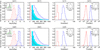 |
Fig. A.1. Same as Figure 2, but for simulation results with and without considering the uncertainties of the two correlations. The panels in the first row are for the simulation results with considering the uncertainties. The panels in the second row are for the simulation results without considering the uncertainties. |
A.7. Reality of the configuration of the gravitational acceleration model
In fact, we must state that we cannot determine the configuration reality of the model, at least at the current stage. Meanwhile, it is difficult to estimate the probability of detecting a merging galaxy pair consisting of an ELG with two NLRs and a non-ELG. Defining this probability would theoretically reduce the likelihood of generating DPNELs shifted in the same direction, since the probability proposed in the manuscript is estimated based on such a dual-core system model.
Appendix B: Spectroscopic analysis of SDSS J0010
To subtract the host galaxy contributions in the spectrum, which would affect the determinations of emission line features, we adopt the penalized pixel fitting (pPXF) code (Cappellari 2017) to determine the host galaxy features. The pPXF code is an improved simple stellar population (SSP) method that uses stellar population spectra while employing a regularization measurement. We have used the older version of the pPXF code to determine the host galaxy features, all emission lines are masked out during the pPXF-fitting. Figure B.1 shows the SDSS provided spectrum of SDSS J0010 and the best-fitting results of pPXF-determined host galaxy features.
After subtracting the host galaxy contributions, the narrow emission lines around Hα and Hβ, where the Balmer emission lines, [N II], [S II], and [O III] are mainly considered. Two Gaussian functions are applied to describe each emission line, except for Hα and [N II] doublet, which require three Gaussian functions for each of these emission lines due to the possible extended components covered in the spectrum. Through fitting the emission lines simultaneously with the MPFIT package, a Levenberg-Marquardt least-squares minimization technique, we determine the best-fitting results to the emission lines, shown in Figure 4, and then obtain the parameters of the Gaussian components. Therefore, we obtain the measured velocity parameters of DPNELs of SDSS J0010 based on the central wavelengths and corresponding uncertainties of the core components, with blueshifted velocities of -343.32±17.27 km/s and -41.51±36.71 km/s, and a velocity separation of  km/s. Here, the uncertainties are determined by the 1σ errors of the central wavelengths related to the core components. It is worth noting that after carefully checking the reported DPNELs galaxies, SDSS J0010 is covered in Ge et al. (2012) and exhibits DPNELs shifted in the same direction with blueshifted velocities of 44.9±8.4 km/s and 316.3±2.8 km/s, and a velocity separation of 271.4±11.2 km/s in their analysis. Our derived velocity parameters are similar to these literature values.
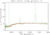 |
Fig. B.1. The rest-frame spectrum of SDSS J0100. The dark green components indicate the SDSS spectrum, while the red components indicate the best-fitting results of the pPXF-determined host galaxy contributions. The mjd-plate-fiberid number of this object and the corresponding χ2/dof related to the best-fitting results are marked in the title. |
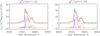 |
Fig. B.2. The best-fitting results to Hα and [N II] emission lines using three Gaussian functions (model B, left panel) to fit each narrow emission line and two Gaussian functions (model A, right panel) to fit each narrow emission line. In both panels, the cyan components represent the spectrum after subtracting the host galaxy features; the thick red components represent the best-fitting results for emission lines; the thin red and thin blue Gaussian components from left to right indicate the double-peaked features of narrow [N II]λ 6550Å, Hα, and [N II]λ 6585Å. In the left panel, the green Gaussian components indicate the extended components of [N II]λ 6550Å, Hα, and [N II]λ 6585Å. In each panel, the corresponding χ2/dof related to the best-fitting results is marked in the title. |
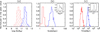 |
Fig. B.3. The parameter distributions for the 218 satisfied runs whose velocity parameters are consistent with SDSS J0010. Panel (a): the histograms filled in red and blue show the logarithmic total stellar mass distributions of the main and companion galaxies. Panel (b): the histograms in red and blue show the distributions of RNLRs and galaxy separation; the distribution of RNLRs/D is shown in the top right region. Panel (c): the histograms filled in red and blue show the distributions of the acceleration duration and orbital period; the distribution of the acceleration duration/orbital period is shown in the top right region. |
We also test whether the model with three Gaussian functions is preferred in fitting Hα and [N II] doublet through the F-test statistical technique. Two models are used to fit Hα and [N II] doublet: model A adopts two Gaussian functions to fit each narrow emission line, and model B adopts three Gaussian functions to fit each narrow emission line. Through the MPFIT package, the best-fitting results of the two models for Hα and [N II] are shown in Figure B.2. Based on the different χ2/dof values for model A and model B (χA2 ∼ 108.5, χB2 ∼ 94.9, dofA ∼ 136, and dofB ∼ 130), the calculated Fp value is about
 (B.1)
(B.1)
where χA2 and χB2 are the sums of squared residuals, and dofA and dofB are the degrees of freedom for model A and model B, respectively. Based on dofA - dofB and dofB as the number of dofs of the F-distribution numerator and denominator, the expected value from the statistical F-test is about 2.94 with a 99% probability. Since Fp = 3.11 > 2.94, it is clarified that the probability is higher than 99% to support the extended components covered in the Hα and [N II] doublet.
Additionally, we also discuss the DPNELs shifted in the same direction of SDSS J0010 by combining our simulation results. Through matching the velocity parameters (± uncertainties) of SDSS J0010 to the satisfied 10,000 simulation trials, we identified 218 runs. The parameter distributions of these 218 simulations are shown in Figure B.3. Since the parameter distributions (masses, galaxy separation, RNLRs, acceleration duration, and orbital period) are dispersive rather than concentrated, it is hard to find a realistically unique set of parameters to interpret the observed DPNELs shifted in the same direction of SDSS J0010 in our simulation results.
Appendix C: Effects of different orbital trajectories
To explore the effects of adopting different orbital trajectories of the two galaxies in the gravitational acceleration model on the simulation results, we performed simulations adopting an elliptical orbital path, with the two galaxies initially positioned at both the apocenter and pericenter, and meanwhile in varying eccentricities. Figure C.1 presents the results for both circular orbits and elliptical orbits with an eccentricity of 0.2. The simulations show small differences between these two cases in the distributions of masses, RNLRs, galaxy separation, acceleration duration, and orbital period. The relationship between eccentricity and mean peak separation of DPNELs shifted in the same direction is shown in Figure C.2. For elliptical orbits with galaxies initially at apocenter, the mean velocity separation decreases with increasing eccentricity, while the opposite relationship occurs for elliptical orbits with galaxies initially at pericenter. Here, the simulations of galaxies initially at apocenter and pericenter with an identical eccentricity share the same semi-major axis. Therefore, since simulations with larger eccentricity result in smaller periapsis distances, the scenario with galaxies initially at pericenter yields no satisfied runs when eccentricity exceeds 0.6.
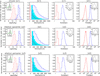 |
Fig. C.1. Same as Figure 2. The panels in the first row display simulation results for a circular orbit. The panels in the second row show simulation results for an elliptical orbit (eccentricity = 0.2) with galaxies initially at apocenter. The panels in the third row present simulation results for an elliptical orbit (eccentricity = 0.2) with galaxies initially at pericenter. |
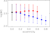 |
Fig. C.2. On the correlation between the eccentricity of an elliptical orbit and the logarithmic mean velocity separation of DPNELs. The solid points in red/blue with corresponding error bars represent the results with galaxies initially at the pericenter/apocenter of the elliptical orbital path. The black point represents the result with a circular orbit (eccentricity = 0). The error bars are calculated using the standard deviation of the corresponding velocity separations. |
All Figures
|
Fig. 1. Diagram of the gravitational acceleration model with the two galaxies initially located at the apocenter of the elliptical orbit. The circles filled in red and blue represent the main and companion galaxies, respectively. The circles filled in yellow represent the NLRs of the main galaxy. The black arrows represent the gravitational force vectors. The green dashed line represents the clockwise elliptical orbit, with θ marking the rotation angle. System I indicates the initial positions of the galaxies in the simulation, aligned along LoS, while system II indicates their final positions. The arrow in the left region marks LoS. |
| In the text | |
|
Fig. 2. Simulation results for the model adopting an elliptical orbit with an eccentricity of 0.2 and with galaxies initially at apocenter. Panel (a): Histograms filled in red and blue show the logarithmic total stellar mass distributions of the main and companion galaxies in the 10 000 satisfied simulations with DPNELs shifted in the same direction. Here, the top left inset displays the mass distributions for the galaxies in the collected main-sample (histogram in purple) and companion-sample (histogram in green). Panel (b): Histograms filled in red, blue, and cyan show the distributions of the smaller blueshifted velocity, larger blueshifted velocity, and velocity separation of DPNELs shifted in the same direction; the arrows in red, blue, and black mark the smaller blueshifted velocity, larger blueshifted velocity, and velocity separation of SDSS J001050.52−103246.6. Panel (c): Histograms in red and blue show the distributions of RNLRs and galaxy separation; the distribution of RNLRs/D is shown in the top right region. Panel (d): Histograms filled in red and blue show the distributions of the acceleration duration and orbital period; the distribution of the acceleration duration/orbital period (t/T) is shown in the top right region. All the histograms are normalized to the peak value. |
| In the text | |
|
Fig. 3. Information on the correlation between L[O III] and logarithmic total stellar mass for the galaxies in the main sample. The green solid line indicates the best-fitting results and the red dashed lines indicate the corresponding 5σ confidence bands. Contour levels in different colors are related to number densities shown in color bar in the top region. |
| In the text | |
|
Fig. 4. Spectroscopic results of SDSS J001050.52−103246.6. Left and right panels present the best-fitting results to the emission lines around Hα and Hβ, respectively. In both panels, the cyan components indicate the spectrum after subtracting the host galaxy starlight; the thick red components indicate the best-fitting results; and the solid lines in the bottom region of each panel indicate residuals. In the left panel, the thin red and thin blue Gaussian components from left to right indicate the double-peaked features of narrow [N II]λ6550 Å, Hα, [N II]λ6585 Å, [S II]λ6718 Å, and [S II]λ6732 Å; the green Gaussian components indicate the extended emission components in [N II]λ6550 Å, Hα, and [N II]λ6585 Å. In the right panel, the thin red and thin blue Gaussian components from left to right indicate the double-peaked features of narrow Hβ, [O III]λ4959 Å, and [O III]λ5007 Å. In each panel, the corresponding χ2/d.o.f. related to the best-fitting results is marked in the title. |
| In the text | |
|
Fig. A.1. Same as Figure 2, but for simulation results with and without considering the uncertainties of the two correlations. The panels in the first row are for the simulation results with considering the uncertainties. The panels in the second row are for the simulation results without considering the uncertainties. |
| In the text | |
|
Fig. B.1. The rest-frame spectrum of SDSS J0100. The dark green components indicate the SDSS spectrum, while the red components indicate the best-fitting results of the pPXF-determined host galaxy contributions. The mjd-plate-fiberid number of this object and the corresponding χ2/dof related to the best-fitting results are marked in the title. |
| In the text | |
|
Fig. B.2. The best-fitting results to Hα and [N II] emission lines using three Gaussian functions (model B, left panel) to fit each narrow emission line and two Gaussian functions (model A, right panel) to fit each narrow emission line. In both panels, the cyan components represent the spectrum after subtracting the host galaxy features; the thick red components represent the best-fitting results for emission lines; the thin red and thin blue Gaussian components from left to right indicate the double-peaked features of narrow [N II]λ 6550Å, Hα, and [N II]λ 6585Å. In the left panel, the green Gaussian components indicate the extended components of [N II]λ 6550Å, Hα, and [N II]λ 6585Å. In each panel, the corresponding χ2/dof related to the best-fitting results is marked in the title. |
| In the text | |
|
Fig. B.3. The parameter distributions for the 218 satisfied runs whose velocity parameters are consistent with SDSS J0010. Panel (a): the histograms filled in red and blue show the logarithmic total stellar mass distributions of the main and companion galaxies. Panel (b): the histograms in red and blue show the distributions of RNLRs and galaxy separation; the distribution of RNLRs/D is shown in the top right region. Panel (c): the histograms filled in red and blue show the distributions of the acceleration duration and orbital period; the distribution of the acceleration duration/orbital period is shown in the top right region. |
| In the text | |
|
Fig. C.1. Same as Figure 2. The panels in the first row display simulation results for a circular orbit. The panels in the second row show simulation results for an elliptical orbit (eccentricity = 0.2) with galaxies initially at apocenter. The panels in the third row present simulation results for an elliptical orbit (eccentricity = 0.2) with galaxies initially at pericenter. |
| In the text | |
|
Fig. C.2. On the correlation between the eccentricity of an elliptical orbit and the logarithmic mean velocity separation of DPNELs. The solid points in red/blue with corresponding error bars represent the results with galaxies initially at the pericenter/apocenter of the elliptical orbital path. The black point represents the result with a circular orbit (eccentricity = 0). The error bars are calculated using the standard deviation of the corresponding velocity separations. |
| In the text | |
Current usage metrics show cumulative count of Article Views (full-text article views including HTML views, PDF and ePub downloads, according to the available data) and Abstracts Views on Vision4Press platform.
Data correspond to usage on the plateform after 2015. The current usage metrics is available 48-96 hours after online publication and is updated daily on week days.
Initial download of the metrics may take a while.