| Issue |
A&A
Volume 699, July 2025
|
|
|---|---|---|
| Article Number | A247 | |
| Number of page(s) | 15 | |
| Section | Planets, planetary systems, and small bodies | |
| DOI | https://doi.org/10.1051/0004-6361/202555289 | |
| Published online | 18 July 2025 | |
Is ozone a reliable proxy for molecular oxygen?
II. The impact of N2O on the O2-O3 relationship for Earth-like atmospheres
1 National Space Institute, Technical University of Denmark,
Elektrovej,
2800
Kgs. Lyngby,
Denmark
2 Instituto de Astrofísica de Andalucía – CSIC,
Glorieta de la Astronomía s/n,
18008
Granada,
Spain
3 School of Physics and Astronomy, University of Southampton,
Highfield,
Southampton
SO17 1BJ,
UK
4 School of Ocean and Earth Science, University of Southampton,
Southampton
SO14 3ZH,
UK
★ Corresponding author.
Received:
24
April
2025
Accepted:
27
May
2025
Abstract
Molecular oxygen (O2) will be an important molecule in the search for biosignatures in terrestrial planetary atmospheres in the coming decades. In particular, O2 combined with a reducing gas (e.g., methane) is considered strong evidence for disequilibrium caused by surface life. However, there are circumstances where it would be very difficult or impossible to detect O2, in which case it has been suggested that ozone (O3), the photochemical product of O2, could be used instead. Unfortunately, the O2-O3 relationship is highly nonlinear and dependent on the host star, as shown in detail in the first paper of this series. This paper further explores the O2-O3 relationship around G0V-M5V host stars, using climate and photochemistry modeling to simulate atmospheres while varying abundances of O2 and nitrous oxide (N2O). Nitrous oxide is of particular importance to the O2-O3 relationship not only because it is produced biologically, but because it is the primary source of nitrogen oxides (NOx), which fuel the NOx catalytic cycle, which destroys O3 and the smog mechanism that produces O3. In our models we varied the O2 mixing ratio from 0.01–150% of the present atmospheric level (PAL) and N2O abundances of 10% and 1000% PAL. We find that varying N2O impacts the O2-O3 relationship differently depending strongly on both the host star and the amount of atmospheric O2. Planets orbiting hotter hosts with strong UV fluxes efficiently convert N2O into NOx, often depleting a significant amount of O3 via faster NOx catalytic cycles. However, for cooler hosts and low O2 levels we find that increasing N2O can lead to an increase in overall O3 due to the smog mechanism producing O3 in the lower atmosphere. Variations in O3 result in significant changes in the amount of harmful UV reaching the surfaces of the model planets as well as the strength of the 9.6 µm O3 emission spectral feature, demonstrating potential impacts on habitability and future observations.
Key words: astrobiology / planets and satellites: atmospheres / planets and satellites: terrestrial planets / planetary systems
© The Authors 2025
 Open Access article, published by EDP Sciences, under the terms of the Creative Commons Attribution License (https://creativecommons.org/licenses/by/4.0), which permits unrestricted use, distribution, and reproduction in any medium, provided the original work is properly cited.
This article is published in open access under the Subscribe to Open model. This email address is being protected from spambots. You need JavaScript enabled to view it. to support open access publication.
1 Introduction
Numerous studies have suggested the use of ozone (O3) as a proxy for molecular oxygen (O2) in recent decades (e.g., Léger et al. 1993; Des Marais et al. 2002; Segura et al. 2003; Léger et al. 2011; Meadows et al. 2018b). This is largely because O2 when combined with a reducing species such as methane (CH4), is considered a strong disequilibrium biosignature. Observing both in a terrestrial planetary atmosphere indicates that strong replenishing fluxes of O2 and CH4 must be present. Currently, life is the only known mechanism capable of providing these replenishing fluxes (e.g., Lovelock 1965; Lederberg 1965; Lippincott et al. 1967; Meadows 2017). Ozone comes into the picture because there are scenarios in which O2 would be very difficult or impossible to detect in a planetary atmosphere when O3 is readily detectable. For example, the mid-IR is an excellent wavelength range for atmospheric characterization, due to the strong spectral features of potential biosignatures (e.g., Quanz et al. 2022; Angerhausen et al. 2024) along with the lessened impact of clouds in planetary emission spectra (e.g., Kitzmann et al. 2011). However, there are no strong O2 features in the mid-IR – only a collisionally induced absorption feature, which is sensitive only to large amounts of abiotically produced O2, not to the smaller amounts indicative of life (Fauchez et al. 2020). Another example considers a planetary atmosphere resembling the low O2 environment of early Earth, rather than the oxygen-rich atmosphere of modern Earth (O2 comprising 21% of the atmosphere). Observing a planet with O2 abundances expected from the Proterozoic era on Earth (2.4–0.54 Gyr ago) O2 would be difficult to detect, while O3 may be detected at trace amounts (e.g., Kasting et al. 1985; Léger et al. 1993; Des Marais et al. 2002; Segura et al. 2003; Léger et al. 2011). For these reasons O3 has been seen as a good alternative to O2.
However, although O3 is the photochemical product of O2, it has also been known for decades that the O2-O3 relationship is highly nonlinear, due to both the pressure and temperature dependency of O3 formation and the requirement of UV for O2 photolysis. To study this further, in the previous paper of this series, Kozakis et al. (2022), we performed atmospheric modeling of Earth-like planets for a range of O2 abundances and a variety of host stars. Here, we use the term “Earth-like” to refer to a terrestrial planet that is the same size and density as Earth, possesses a similar atmospheric composition, and orbits at a distance where it receives the same total flux from its host star as modern Earth. In our first study, we varied the atmospheric abundance of O2 from 0.01–150% PAL (present atmospheric level) around G0V-M5V host stars. We found that the O2-O3 relationship was extremely influenced by the host star, with planets around hotter stars (G0V-K2V) following different trends to those around cooler stars (K5V-M5V). Planets around hotter stars reached their peak O3 abundance at O2 levels of just 25– 55% PAL, with the Earth-Sun system having a similar amount of O3 at both 10% and 100% PAL O2. This was due to the pressure dependency of O3 formation, an effect first discussed in Ratner & Walker (1972), although our previous study was the first to replicate it using modern atmospheric models and host stars other than the Sun. Cooler stars, on the other hand, were shown to host planets on which O3 decreased along with O2. Additionally, we found that the amount of UV reaching the planetary surface varied nonlinearly with both incoming UV and O3, and that O3 features in simulated emission spectra depended more strongly on atmospheric temperature profiles than on the actual amount of O3 (or O2) in the atmosphere. Already from that study, we determined that using O3 as a proxy for O2 would require knowledge of the host star spectrum, climate and photochemistry modeling, and general atmospheric context. For planets around hotter hosts, another layer of complexity exists, due to the fact that similar O3 abundances can occur at very different O2 values, making it impossible to glean the total O2 abundance from a measurement of only total O3 abundance. However, O3 measurements could still provide useful information on the atmosphere and potentially give insight into whether life could exist on the planetary surface. This paper is a continuation of that study, specifically focusing on how O2-O3 relationships could vary with different atmospheric compositions.
In this current study, we expand upon the models from Kozakis et al. (2022) by varying not only O2 but also nitrous oxide (N2O). Nitrous oxide is particularly interesting in this context, not only because it is biologically produced and considered a promising biosignature (e.g., Schwieterman et al. 2018; Angerhausen et al. 2024), but also because it is the “parent species” of nitrogen oxides (NOx). These nitrogen oxides play a crucial role in the two catalytic cycles that destroy O3 as well as the smog mechanism that produces O3.
Since the rate at which N2O is converted into NOx is dependent on photolysis rates, the degree to which varying N2O impacts the O2-O3 relationship depends on both the overall spectrum of the host star as well as the UV spectral slope. This paper includes all of the models from Kozakis et al. (2022), rerun with different amounts of N2O. Section 2 reviews the relevant chemistry of O3 and N2O, and Sect. 3 describes the atmospheric models, the input stellar spectra, and the radiative transfer model. Section 4 analyzes how varying N2O alters atmospheric chemistry, surface UV flux, and simulated planetary emission spectra. Section 5 compares this to similar studies and discusses atmospheric parameters, which affect N2O abundances in Earth-like planetary atmospheres. A summary of the study and conclusions are available in Sect. 6.
2 Relevant chemistry
2.1 Ozone formation and destruction
The majority of O3 on Earth is formed via the Chapman mechanism (Chapman 1930), beginning with O2 photolysis creating atomic O, which then combines with another O2 molecule with the help of a background molecule, M, to carry away the excess energy:
![Mathematical equation: \[\frame{\frame{\text{O}}_\frame{\text{2}}}\frame{\text{~ + ~h}}\nu \, \to \,\frame{\text{O~ + ~O~(175~ < ~}}\lambda \,\frame{\text{ < ~242~nm),}}\]](/articles/aa/full_html/2025/07/aa55289-25/aa55289-25-eq1.png) (1)
(1)
![Mathematical equation: \[\frame{\text{O}}\, + \,\frame{\frame{\text{O}}_\frame{\text{2}}}\frame{\text{~ + ~}}M\, \to \,\frame{\frame{\text{O}}_\frame{\text{3}}}\frame{\text{~ + ~}}M.\]](/articles/aa/full_html/2025/07/aa55289-25/aa55289-25-eq2.png) (2)
(2)
Since Reaction (2) is a three-body reaction, it proceeds faster at higher atmospheric densities, with this reaction in particular having a strong temperature dependence, favoring cooling temperatures. While Reaction (1) creates ground state O atoms (also written as O(3P)), the O2 photolysis initiated by photons with wavelengths less than 175 nm creates the O(1D) radical,
![Mathematical equation: \[\frame{O_2}~ + ~\frame{\text{h}}v\, \to \,O~ + ~O\frame{(^1}D)~(~\lambda \, < ~175~nm),\]](/articles/aa/full_html/2025/07/aa55289-25/aa55289-25-eq3.png) (3)
(3)
which can then be quenched back to the ground state via collisions with a background molecule,
![Mathematical equation: \[\frame{\text{O}}\frame{(^1}\frame{\text{D)}}\, + \,M\, \to \,\frame{\text{O}}\, + \,M,\]](/articles/aa/full_html/2025/07/aa55289-25/aa55289-25-eq4.png) (4)
(4)
or react with other molecules. Similarly O3 photolysis creates O2 and either a ground O atom or an excited O(1D) radical depending on the energy level of the photon:
![Mathematical equation: \[\frame{\frame{\text{O}}_3}\, + \,\frame{\text{h}}\nu \, \to \,\frame{\frame{\text{O}}_2}\, + \,\frame{\text{O}}\frame{\frame{\text{(}}^\frame{\text{1}}}\frame{\text{D)(}}\lambda \,\frame{\text{ < }}\,\frame{\text{310}}\,\frame{\text{nm),}}\]](/articles/aa/full_html/2025/07/aa55289-25/aa55289-25-eq5.png) (5)
(5)
![Mathematical equation: \[\frame{\frame{\text{O}}_3}\, + \,\frame{\text{h}}\nu \, \to \,\frame{\frame{\text{O}}_2}\, + \,\frame{\text{O}}\,\frame{\text{(310}}\,\frame{\text{ < }}\,\lambda \,\frame{\text{ < }}\,\frame{\text{1140}}\,\frame{\text{nm)}}\frame{\text{.}}\]](/articles/aa/full_html/2025/07/aa55289-25/aa55289-25-eq6.png) (6)
(6)
After photolysis the resulting O atom often recombines with O2 via Reaction (2), so the photolysis of O3 is not seen as a loss of O3. Due to the constant cycling between O3 and O, it is often useful to keep track of O + O3, termed “odd oxygen”, rather than tracking both individually. Odd oxygen can be lost when converted to O2 molecules, as seen in,
![Mathematical equation: \[\frame{\frame{\text{O}}_3}\, + \,\frame{\text{O}} \to \,2\frame{\frame{\text{O}}_2}\frame{\text{.}}\]](/articles/aa/full_html/2025/07/aa55289-25/aa55289-25-eq7.png) (7)
(7)
The conversion of odd oxygen back into O2 requires the Chapman mechanism to restart with O2 photolysis, which is the slowest and limiting reaction of O3 formation. However, Reaction (7) is significantly slower, so O from O3 photolysis tends to preferentially combine with O2 back into O3 (Reaction (2)). On Earth the majority of O3 is created via the Chapman mechanism, with formation rates highest in the stratosphere. This region is high enough in the atmosphere that O2 is quickly photolyzed, yet still has sufficient atmospheric density for the three-body reaction that creates O3 (Reaction (2)) to be efficient.
Lower in the atmosphere, primarily in the troposphere, there is another mechanism for O3 formation, which is referred to as “smog formation” (Haagen-Smit 1952), expressed as,
![Mathematical equation: \[\frame{\text{OH}}\, + \,\frame{\text{CO}} \to \,\frame{\text{H~ + ~C}}\frame{\frame{\text{O}}_\frame{\text{2}}},\]](/articles/aa/full_html/2025/07/aa55289-25/aa55289-25-eq8.png) (8)
(8)
![Mathematical equation: \[\frame{\text{H~ + ~}}\frame{\frame{\text{O}}_\frame{\text{2}}}\frame{\text{~ + ~}}M\, \to \,\frame{\text{H}}\frame{\frame{\text{O}}_\frame{\text{2}}}\frame{\text{~ + ~}}M\frame{\text{,}}\]](/articles/aa/full_html/2025/07/aa55289-25/aa55289-25-eq9.png) (9)
(9)
![Mathematical equation: \[\frame{\text{H}}\frame{\frame{\text{O}}_\frame{\text{2}}}\frame{\text{~ + ~NO}}\, \to \,\frame{\text{OH~ + ~N}}\frame{\frame{\text{O}}_\frame{\text{2}}}\frame{\text{,}}\]](/articles/aa/full_html/2025/07/aa55289-25/aa55289-25-eq10.png) (10)
(10)
![Mathematical equation: \[\frame{\text{N}}\frame{\frame{\text{O}}_\frame{\text{2}}}\frame{\text{~ + ~h}}\nu \, \to \,\frame{\text{NO~ + ~O,}}\]](/articles/aa/full_html/2025/07/aa55289-25/aa55289-25-eq11.png) (11)
(11)
![Mathematical equation: \[\frame{\text{O~ + ~}}\frame{\frame{\text{O}}_\frame{\text{2}}}\frame{\text{~ + ~}}M\, \to \,\frame{\frame{\text{O}}_\frame{\text{3}}}\frame{\text{~ + ~}}M\frame{\text{.}}\]](/articles/aa/full_html/2025/07/aa55289-25/aa55289-25-eq12.png) (2)
(2)
![Mathematical equation: \[\overline \frame{\frame{\text{Net}}:\frame{\text{~CO}}\, + \,\frame{\text{2}}\frame{\frame{\text{O}}_\frame{\text{2}}}\, + \,\frame{\text{h}}\nu \, \to \,\frame{\text{C}}\frame{\frame{\text{O}}_\frame{\text{2}}}\, + \,\frame{\frame{\text{O}}_\frame{\text{3}}}} \]](/articles/aa/full_html/2025/07/aa55289-25/aa55289-25-eq13.png)
This chain of reactions requires hydrogen oxides ![Mathematical equation: \[(\frame{\text{H}}\frame{\frame{\text{O}}_x},\,\frame{\text{H}}\frame{\frame{\text{O}}_\frame{\text{2}}}\overset{}{\mathop + } \,\frame{\text{OH}}\,\frame{\text{ + }}\,\frame{\text{H}})\]](/articles/aa/full_html/2025/07/aa55289-25/aa55289-25-eq14.png) and nitrogen oxides (NOx, NO3 + NO2 + NO) as catalysts, although they are not consumed. On Earth the smog mechanism is slower and produces significantly less O3 than the Chapman mechanism, but studies such as Grenfell et al. (2013) have demonstrated that planets around cooler spectral hosts may experience much higher efficiency in the smog mechanism.
and nitrogen oxides (NOx, NO3 + NO2 + NO) as catalysts, although they are not consumed. On Earth the smog mechanism is slower and produces significantly less O3 than the Chapman mechanism, but studies such as Grenfell et al. (2013) have demonstrated that planets around cooler spectral hosts may experience much higher efficiency in the smog mechanism.
While the Chapman and smog mechanisms are the main sources of O3 formation, catalytic cycles are the main sources of O3 destruction. These are cycles in which there is a net loss of odd oxygen as follows,
![Mathematical equation: \[\begin{array}{{c}} \frame{\,\,\,\frame{\text{X~ + ~}}\frame{\frame{\text{O}}_\frame{\text{3}}} \to \frame{\text{XO~ + }}\,\frame{\frame{\text{O}}_\frame{\text{2}}}\frame{\text{,}}} \hfill \\ \frame{\,\,\,\,\,\frame{\text{XO}}\,\frame{\text{ + }}\,\frame{\text{O}}\, \to \,\frame{\text{X}}\,\frame{\text{ + }}\,\frame{\frame{\text{O}}_\frame{\text{2}}}\frame{\text{,}}} \hfill \\ \frame{\overline \frame{\frame{\text{Net:~}}\,\,\,\,\frame{\frame{\text{O}}_\frame{\text{3}}}\,\frame{\text{ + }}\,\frame{\text{~O}}\, \to \,\frame{\text{2}}\frame{\frame{\text{O}}_\frame{\text{2}}}} } \hfill \\ \end{array} \]](/articles/aa/full_html/2025/07/aa55289-25/aa55289-25-eq15.png)
with X and XO cycling between each other without loss. On Earth the two most dominant cycles use X = NO and X = OH for the NOx and HOx catalytic cycles, respectively. The HOx catalytic cycle is as follows,
![Mathematical equation: \[\frame{\text{OH~ + ~}}\frame{\frame{\text{O}}_\frame{\text{3}}}\, \to \,\frame{\text{H}}\frame{\frame{\text{O}}_\frame{\text{2}}}\,\frame{\text{ + }}\,\frame{\frame{\text{O}}_\frame{\text{2}}}\frame{\text{,}}\]](/articles/aa/full_html/2025/07/aa55289-25/aa55289-25-eq16.png) (12)
(12)
![Mathematical equation: \[\frame{\text{H}}\frame{\frame{\text{O}}_\frame{\text{2}}}\frame{\text{~ + ~O~}} \to \frame{\text{OH~ + ~}}\frame{\frame{\text{O}}_\frame{\text{2}}}\frame{\text{,}}\]](/articles/aa/full_html/2025/07/aa55289-25/aa55289-25-eq17.png) (13)
(13)
in which odd oxygen, O + O3, is converted into two O2. In the upper stratosphere where H atoms are more common (often from H2O photolysis) odd oxygen can be converted to O2 via,
![Mathematical equation: \[\frame{\text{H~ + ~}}\frame{\frame{\text{O}}_\frame{\text{2}}}\frame{\text{~ + ~}}M\frame{\text{~}} \to \frame{\text{H}}\frame{\frame{\text{O}}_\frame{\text{2}}}\frame{\text{~ + ~}}M\frame{\text{,}}\]](/articles/aa/full_html/2025/07/aa55289-25/aa55289-25-eq18.png) (14)
(14)
![Mathematical equation: \[\frame{\text{H}}\frame{\frame{\text{O}}_\frame{\text{2}}}\frame{\text{~ + ~O~}} \to \frame{\text{~OH~ + ~}}\frame{\frame{\text{O}}_\frame{\text{2}}}\frame{\text{,}}\]](/articles/aa/full_html/2025/07/aa55289-25/aa55289-25-eq19.png) (13)
(13)
![Mathematical equation: \[\frame{\text{OH~ + ~O}} \to \frame{\text{~H~ + ~O}}\frame{\text{.}}\]](/articles/aa/full_html/2025/07/aa55289-25/aa55289-25-eq20.png) (15)
(15)
In the lower stratosphere where there is less O2 photolysis and therefore fewer O atoms, odd oxygen is destroyed via,
![Mathematical equation: \[\frame{\text{OH~ + ~}}\frame{\frame{\text{O}}_\frame{\text{3}}}\frame{\text{~}} \to \frame{\text{H}}\frame{\frame{\text{O}}_\frame{\text{2}}}\frame{\text{~ + ~}}\frame{\frame{\text{O}}_\frame{\text{2}}}\frame{\text{,}}\]](/articles/aa/full_html/2025/07/aa55289-25/aa55289-25-eq21.png) (16)
(16)
![Mathematical equation: \[\frame{\text{H}}\frame{\frame{\text{O}}_\frame{\text{2}}}\frame{\text{~ + ~}}\frame{\frame{\text{O}}_\frame{\text{3}}}\frame{\text{~}} \to \frame{\text{~OH~ + ~2}}\frame{\frame{\text{O}}_\frame{\text{2}}}\frame{\text{.}}\]](/articles/aa/full_html/2025/07/aa55289-25/aa55289-25-eq22.png) (17)
(17)
There are multiple reactions that destroy either OH or HO2, but they are typically recycled back into another HOx species. Photolysis is also not a true sink of HOx, since HO2 photolysis creates OH, and OH is too short-lived for significant photolysis. Efficient methods of HOx destruction include conversion to H2O,
![Mathematical equation: \[\frame{\text{OH~ + ~H}}\frame{\frame{\text{O}}_\frame{\text{2}}} \to \frame{\text{~}}\frame{\frame{\text{H}}_\frame{\text{2}}}\frame{\text{O~ + ~}}\frame{\frame{\text{O}}_\frame{\text{2}}}\frame{\text{,}}\]](/articles/aa/full_html/2025/07/aa55289-25/aa55289-25-eq23.png) (18)
(18)
or conversion to a stable reservoir species, such as
![Mathematical equation: \[\frame{\text{OH}}\,\frame{\text{ + }}\,\frame{\text{OH}}\,\frame{\text{ + }}\,M\, \to \,\frame{\frame{\text{H}}_2}\frame{\frame{\text{O}}_\frame{\text{2}}}\, + \,M,\]](/articles/aa/full_html/2025/07/aa55289-25/aa55289-25-eq24.png) (19)
(19)
![Mathematical equation: \[\frame{\text{OH}}\,\frame{\text{ + }}\,\frame{\text{N}}\frame{\frame{\text{O}}_\frame{\text{2}}}\,\frame{\text{ + }}\,M\, \to \,\frame{\text{HN}}\frame{\frame{\text{O}}_\frame{\text{3}}}\, + \,M,\]](/articles/aa/full_html/2025/07/aa55289-25/aa55289-25-eq25.png) (20)
(20)
![Mathematical equation: \[\frame{\text{H}}\frame{\frame{\text{O}}_2}\,\frame{\text{ + }}\,\frame{\text{N}}\frame{\frame{\text{O}}_\frame{\text{2}}}\,\frame{\text{ + }}\,M\, \to \,\frame{\text{H}}\frame{\frame{\text{O}}_2}\frame{\text{N}}\frame{\frame{\text{O}}_\frame{\text{2}}}\, + \,M.\]](/articles/aa/full_html/2025/07/aa55289-25/aa55289-25-eq26.png) (21)
(21)
The other primary catalytic cycle, the NOx catalytic cycle, is discussed in the next subsection, as it is fueled by N2O.
2.2 Nitrous oxide and NOx catalytic cycles
Nitrous oxide, considered itself a biosignature, is primarily created by nitrification and denitrification processes in soils and oceans, with very few abiotic sources. On Earth there are additionally many anthropogenic sources of N2O, mainly from agricultural processes. The only known major sink of N2O is photolysis in the stratosphere. N2O photolysis is one of the sources of the O(1D) radical,
![Mathematical equation: \[\frame{\frame{\text{N}}_\frame{\text{2}}}\frame{\text{O~ + ~h}}\nu \, \to \,\frame{N_2} + \,\frame{\text{O}}\frame{\frame{\text{(}}^\frame{\text{1}}}\frame{\text{D),}}\]](/articles/aa/full_html/2025/07/aa55289-25/aa55289-25-eq27.png) (22)
(22)
which can react with N2O to create NO,
![Mathematical equation: \[\frame{\frame{\text{N}}_\frame{\text{2}}}\frame{\text{O}}\,\frame{\text{ + }}\,\frame{\text{O}}\frame{\frame{\text{(}}^\frame{\text{1}}}\frame{\text{D)}}\, \to \,\frame{\text{NO}}\, + \,\frame{\text{NO,}}\]](/articles/aa/full_html/2025/07/aa55289-25/aa55289-25-eq28.png) (23)
(23)
or N2 and O2,
![Mathematical equation: \[\frame{\frame{\text{N}}_\frame{\text{2}}}\frame{\text{O}}\,\frame{\text{ + }}\,\frame{\text{O}}\frame{\frame{\text{(}}^\frame{\text{1}}}\frame{\text{D)}}\, \to \,\frame{\frame{\text{N}}_\frame{\text{2}}}\, + \,\,\frame{\frame{\text{O}}_\frame{\text{2}}}.\]](/articles/aa/full_html/2025/07/aa55289-25/aa55289-25-eq29.png) (24)
(24)
While N2O is the main non-anthropogenic source of NOx, there are additionally minor sources of NOx from cosmic rays and lightning (e.g., Nicolet 1975; Tuck 1976; Shumilov et al. 2003; Braam et al. 2022), which are not explored in this study. The primary NOx catalytic cycle working in the stratosphere follows as,
![Mathematical equation: \[\frame{\text{NO}}\,\frame{\text{ + }}\,\frame{\frame{\text{O}}_\frame{\text{3}}}\, \to \,\frame{\text{N}}\frame{\frame{\text{O}}_\frame{\text{2}}}\, + \,\,\frame{\frame{\text{O}}_\frame{\text{2}}},\]](/articles/aa/full_html/2025/07/aa55289-25/aa55289-25-eq30.png) (25)
(25)
![Mathematical equation: \[\frame{\text{N}}\frame{\frame{\text{O}}_2}\,\frame{\text{ + }}\,\frame{\text{O}}\, \to \,\frame{\text{NO}}\, + \,\,\frame{\frame{\text{O}}_\frame{\text{2}}}.\]](/articles/aa/full_html/2025/07/aa55289-25/aa55289-25-eq31.png) (26)
(26)
Nitrate (NO3) is photolyzed at longer wavelengths, allowing NO3 photolysis to occur in the lower stratosphere and further contributing to O3 destruction, as follows,
![Mathematical equation: \[\frame{\text{NO}}\,\frame{\text{ + }}\,\frame{\frame{\text{O}}_\frame{\text{3}}}\, \to \,\frame{\text{N}}\frame{\frame{\text{O}}_\frame{\text{2}}}\, + \,\,\frame{\frame{\text{O}}_\frame{\text{2}}},\]](/articles/aa/full_html/2025/07/aa55289-25/aa55289-25-eq32.png) (25)
(25)
![Mathematical equation: \[\frame{\text{N}}\frame{\frame{\text{O}}_\frame{\text{2}}}\,\frame{\text{ + }}\,\frame{\frame{\text{O}}_\frame{\text{3}}}\, \to \,\frame{\text{N}}\frame{\frame{\text{O}}_\frame{\text{3}}}\, + \,\,\frame{\frame{\text{O}}_\frame{\text{2}}},\]](/articles/aa/full_html/2025/07/aa55289-25/aa55289-25-eq33.png) (27)
(27)
![Mathematical equation: \[\frame{\text{N}}\frame{\frame{\text{O}}_\frame{\text{2}}}\,\frame{\text{ + }}\,\frame{\frame{\text{O}}_\frame{\text{3}}}\, \to \,\frame{\text{N}}\frame{\frame{\text{O}}_\frame{\text{3}}}\, + \,\,\frame{\frame{\text{O}}_\frame{\text{2}}},\]](/articles/aa/full_html/2025/07/aa55289-25/aa55289-25-eq34.png) (28)
(28)
NOx is lost from the atmosphere through reactions with N atoms, as shown below,
![Mathematical equation: \[\frame{\text{NO}}\,\frame{\text{ + }}\,\frame{\text{N}}\, \to \,\frame{\frame{\text{N}}_\frame{\text{2}}}\, + \,\,\frame{\text{O,}}\]](/articles/aa/full_html/2025/07/aa55289-25/aa55289-25-eq35.png) (29)
(29)
where the N atoms are produced by the photolysis of NO:
![Mathematical equation: \[\frame{\text{NO}}\,\frame{\text{ + }}\,\frame{\text{h}}\nu \, \to \,\frame{\frame{\text{N}}_\frame{\text{2}}}\, + \,\,\frame{\text{O}}\frame{\text{.}}\]](/articles/aa/full_html/2025/07/aa55289-25/aa55289-25-eq36.png) (30)
(30)
Other sinks include conversion to reservoir species, as shown by
![Mathematical equation: \[\frame{\text{N}}\frame{\frame{\text{O}}_2}\,\frame{\text{ + }}\,\frame{\text{N}}\frame{\frame{\text{O}}_\frame{\text{3}}}\, + \,M\, \to \,\frame{\frame{\text{N}}_\frame{\text{2}}}\frame{\frame{\text{O}}_\frame{\text{5}}}\, + \,M,\]](/articles/aa/full_html/2025/07/aa55289-25/aa55289-25-eq37.png) (31)
(31)
![Mathematical equation: \[\frame{\text{OH}}\,\frame{\text{ + }}\,\frame{\text{N}}\frame{\frame{\text{O}}_\frame{\text{2}}}\, + \,M\, \to \,\frame{\text{HN}}\frame{\frame{\text{O}}_\frame{\text{3}}}\, + \,M,\]](/articles/aa/full_html/2025/07/aa55289-25/aa55289-25-eq38.png) (20)
(20)
![Mathematical equation: \[\frame{\text{H}}\frame{\frame{\text{O}}_2}\,\frame{\text{ + }}\,\frame{\text{N}}\frame{\frame{\text{O}}_\frame{\text{2}}}\, + \,M\, \to \,\frame{\text{H}}\frame{\frame{\text{O}}_2}\frame{\text{N}}\frame{\frame{\text{O}}_\frame{\text{2}}}\, + \,M,\]](/articles/aa/full_html/2025/07/aa55289-25/aa55289-25-eq39.png) (21)
(21)
in which the reservoir species are significantly less reactive.
2.3 NOx-limited and NOx-saturated regimes
Since the smog mechanism uses O atoms created by NO2 photolysis to create O3, it might seem that an increase in NOx in the lower atmosphere would always lead to a faster smog mechanism. However, the relationship between NOx and the smog mechanism is complicated due to the relationship between NOx and HOx. While NOx is produced from N2O in the atmosphere, HOx is often indirectly created from O3 itself. Hydroxyl (OH) is most commonly created by oxidation of water with the O(1D) radical,
![Mathematical equation: \[\frame{\text{H}}\frame{\frame{\text{O}}_2}\,\frame{\text{ + }}\,\frame{\text{O}}\frame{\frame{\text{(}}^\frame{\text{1}}}\frame{\text{D)}}\, \to \,\frame{\text{OH}}\,\frame{\text{ + }}\,\frame{\text{OH,}}\]](/articles/aa/full_html/2025/07/aa55289-25/aa55289-25-eq40.png) (32)
(32)
with the majority of O(1D) in the lower atmosphere created from O3 photolysis (Reaction (5)). Therefore, an increase in O3 often leads to an increase in HOx. It follows that an increase in NOx would allow increased smog production of O3, with the higher O3 concentrations creating more HOx. However, this only holds true in what we call a “NOx-limited” regime, where increasing NOx leads to an increase in HOx. Sufficiently high levels of NOx will induce a shift into what we call the “NOx-saturated” regime, where NOx will become efficient at locking up HOx into reservoir species such as HNO3 and HO2NO2 (Reactions (20) and (21)). This relationship in the NOx-limited and NOx-saturated regimes as they exist for modern Earth is shown in Fig. 1. Since NOx and HOx are primarily created through reactions of O(1D) with N2O and H2O, respectively (Reactions (23,32)), and O(1D) is created via photolysis, the amount of incoming UV from the host star plays a crucial role in determining which NOx regime is dominant in the atmosphere.
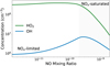 |
Fig. 1 Impact of HO2 and OH in the NOx-limited and NOx-saturated regimes on modern Earth, adapted from Logan et al. (1981). In the NOx-limited regime (white background), increasing NOx allows for a more efficient smog mechanism, with the resulting increase in O3 causing a corresponding rise in HOx. In the NOx-saturated regime (gray background), the abundance of NOx rises to the point where smog O3 production is suppressed as NOx depletes HOx (a necessary catalyst for the smog mechanism) by locking it up into reservoir species. |
3 Methods
3.1 Atmospheric models
We used Atmos1, a publicly available 1D coupled climate and photochemistry code for atmospheric modeling, following Kozakis et al. (2022). Here, we give a brief summary of the code, with more details available in other papers (Arney et al. 2016; Meadows et al. 2018a; Kozakis et al. 2022). For inputs Atmos requires a stellar host spectrum (121.6–45 450 nm), upper and lower boundary conditions for individual gases, initial concentrations of gaseous species, and planetary parameters (radius, gravity, and surface albedo).
We used the modern Earth template for the photochemistry code (Kasting 1979; Zahnle et al. 2006), which contains 50 gaseous species and a network of 233 chemical reactions. The atmosphere was calculated up to 100 km and was broken up into 200 plane parallel layers, each solving the flux and continuity equations simultaneously to determine the atmospheric composition. Vertical transport was included for all the species that were not considered “short-lived,” including molecular and eddy diffusion. Radiative transfer calculations used the δ-2-stream method developed in Toon et al. (1989), and convergence was reached when the adaptive time step reached the age of the universe (∼1017 seconds) within the first 100 steps of the code.
The climate model (Kasting & Ackerman 1986; Kopparapu et al. 2013; Arney et al. 2016) calculates the temperature and pressure profile of the atmosphere based on the incoming stellar radiation and the atmospheric composition. As with the photochemistry code, a δ-2-stream multiple scattering method computes the absorption of stellar flux throughout the atmosphere, and then a correlated-k method computes the absorption of O3, H2O, CH4, CO2, and C2H6 in each layer for outgoing IR radiation including both single and multiple scattering. The atmosphere was broken up into 100 layers from the surface up until 1 mbar (typically <60–70 km), as the code could not be reliably run above these pressures (Arney et al. 2016). Temperatures and species profiles were held constant above this altitude when transferred to the photochemistry code. Convergence was achieved when the temperature and flux differences out of the top of the atmosphere were deemed sufficiently small (<10−5) (Arney et al. 2016).
We ran the climate and photochemistry models, coupled using the “short-stepping” convergence method (Teal et al. 2022; Kozakis et al. 2022), iterating back and forth for 30 iterations or until convergence for the two codes was reached. For this study we explored “Earth-like” atmospheres around a variety of host stars, with varying constant mixing ratios of O2 and N2O, building off of Kozakis et al. (2022), who modeled only variations in O2. As in Kozakis et al. (2022) we used modern Earth initial conditions for our model atmospheres and varied O2 from 0.01– 150% PAL. Lower O2 values were not explored because they are likely unstable Gregory et al. (2021), and higher values similarly were not explored as they are not compatible with life due to O2 combustibility (Kump 2008). All our model planets were run at the Earth-equivalent distance, with a surface pressure of 1 bar, the radius of Earth, and initial gaseous species abundances as listed in the modern Earth Atmos template. This study used all the models from Kozakis et al. (2022) with high and low N2O models using 1000 and 10% PAL N2O, respectively (see Table 1). Fixed mixing ratios of N2O were used (with the modern value of N2O=3.0 × 10⁻⁷), to better isolate the effects on O3. These values were picked in order to begin mapping out the parameter space of atmospheres with different biological fluxes and their impact on O3 at different O2 levels. Since we delved into the O2-O3 relationship for changing only O2 in Kozakis et al. (2022), this paper primarily focuses on how changes in N2O impact O3 levels and the atmosphere generally in comparison to the models with modern levels of N2O.
Model parameters.
3.2 Input stellar spectra
The same Atmos input stellar spectra from Kozakis et al. (2022) were used, with hosts ranging from G0V-M5V (for more details, see Kozakis et al. 2022). The G0V-K5V stellar spectra were originally created in Rugheimer et al. (2015) and consist of UV data from International Ultraviolet Explorer (IUE) data archives2 combined with ATLAS spectra (Kurucz 1979) for the visible and IR wavelength regions. For the M5V star, we used UV data of GJ 876 from the Measurements of the Ultraviolet Spectral Characteristics of Low-mass Exoplanetary Eystems (MUSCLES) survey (France et al. 2016). The UV spectra of all host stars are shown in Fig. 2 along with a comparison to cross sections of gaseous species relevant to O3 formation and destruction. The UV spectrum is important for O3 formation, particularly the UV spectral slope of the far-UV (FUV; λ < 200 nm) and mid- and near-UV (abbreviated NUV, for brevity; 200 nm < λ < 400 nm), with later stars tending to have higher FUV/NUV ratios due to activity and high NUV absorption via TiO (Harman et al. 2015).
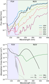 |
Fig. 2 UV stellar spectra of the host stars in this study (top) and corresponding absorption cross sections of relevant gaseous species (bottom). The two plots cover the same wavelength range in order to facilitate comparisons. Cross sections for NO2 and N2O are cut off at shorter wavelengths, due to the dominance of absorption from CO2 and other atmospheric species. |
3.3 Post-processing radiative transfer models
We used the Planetary Intensity Code for Atmospheric Scattering Observations (PICASO) to compute planetary emission spectra from our atmospheric models (Batalha et al. 2019, 2021), following Kozakis et al. (2022). This code is publicly available3 with the ability to compute transmission, reflectance, and emission spectra. For emission spectra we input atmospheric profiles of gaseous species and T/P profiles from Atmos and run our models at a phase angle 0° (full phase) for wavelengths of 0.3–14 µm. We focus in particular on the 9.6 µm O3 feature.
4 Results
Here, we explore the results of our planetary atmospheric models for high and low N2O and compare them to the Kozakis et al. (2022) atmospheric models with modern levels of N2O. The impact of varying N2O levels on the O2-O3 relationship is shown to be nonlinear in all cases, with a strong dependency on both the stellar host and the amount of atmospheric O2. In Sect. 4.1 we analyze the atmospheric chemistry of the varying N2O models, the variations in UV to the ground in Sect. 4.2, and the resulting planetary emission spectra in Sect. 4.3. Additional supporting figures and tables are available in Appendix A.
4.1 Atmospheric chemistry
4.1.1 Atmospheric chemistry: Overview
Changing N2O is shown to have varying effects on the O2-O3 relationship depending on the O2 level and stellar host, with stronger effects seen with high N2O models when compared to the low N2O models. Results for O3 abundances normalized to modern levels of N2O with the high and low N2O models at 100%, 10%, 1%, and 0.1% PAL O2 for all hosts are in Fig. 3, with absolute O3 values for all O2 levels modeled for the Sun- and M5V-hosted planets in Fig. 4. Absolute O3 results for planets around all hosts at all modeled N2O and O2 levels with a comparison to results from Kozakis et al. (2022) are located in the Appendix (Fig. A.1). For planets around all hosts at O2 levels near 100% PAL there is a decrease in O3 for high N2O, and an increase in O3 for low N2O. Planets hosted by all stars except the coolest one (M5V) experience a large amount of O3 depletion at O2 levels similar to modern Earth for the high N2O models, with K2V having the overall largest depletion at 100% PAL, only retaining 47% of its O3 when compared to models with modern levels of N2O. In contrast for the corresponding model for the M5V-hosted planet 95% of the original O3 remains.
For the low N2O models at 100% PAL O2 the planets around both the Sun and the K2V host are most impacted, with O3 abundances of 129% of the O3 they had with modern N2O levels. Again, the planet around the M5V host is least affected, with 103% of the O3 compared to results from modern N2O levels. At low O2 levels for the high N2O models planets around all hosts experience an increase in O3, with this effect being most significant for the planet around the M5V host. The main factors at work determining the impact of N2O on O3 abundance are:
the balance between the host star’s ability to convert N2O into NOx and to destroy N2O via photolysis
whether the amount of NOx reaches the threshold to enter the NOx-saturated regime, which inhibits the smog mechanism
Both of these concepts are discussed at length in the following subsections.
4.1.2 Atmospheric chemistry: Efficiency of conversion of N2O into NOx and N2O photolysis
The degree to which varying N2O impacts O3 abundance is largely dependent on the host stars’ ability to convert N2O into NOx, as well as the rate at which N2O is destroyed via photolysis. Although N2O levels are the same for planets around all host stars, the rate at which the incoming host star flux converts N2O to NOx varies based on the UV spectrum of the host. Conversion of N2O into NOx requires an O(1D) radical (Reaction (23)), which is created via,
![Mathematical equation: \[\frame{\frame{\text{O}}_\frame{\text{2}}}\, + \,\frame{\text{h}}\nu \, \to \,\frame{\text{O}}\,\frame{\text{ + }}\,\frame{\text{O}}\frame{\frame{\text{(}}^\frame{\text{1}}}\frame{\text{D)}}\,(\lambda \, < \,175\,\frame{\text{nm}}),\]](/articles/aa/full_html/2025/07/aa55289-25/aa55289-25-eq41.png) (3)
(3)
![Mathematical equation: \[\frame{\frame{\text{O}}_\frame{\text{3}}}\, + \,\frame{\text{h}}\nu \, \to \,\frame{\frame{\text{O}}_\frame{\text{2}}}\,\frame{\text{ + }}\,\frame{\text{O}}\frame{\frame{\text{(}}^\frame{\text{1}}}\frame{\text{D)}}\,(\lambda \, < \,310\,\frame{\text{nm}}),\]](/articles/aa/full_html/2025/07/aa55289-25/aa55289-25-eq42.png) (5)
(5)
![Mathematical equation: \[\frame{\frame{\text{N}}_\frame{\text{2}}}\frame{\text{O~ + ~h}}\nu \, \to \,\frame{\frame{\text{N}}_\frame{\text{2}}}\, + \,\frame{\text{O}}\frame{\frame{\text{(}}^\frame{\text{1}}}\frame{\text{D)}}\,(\lambda \, < \,200\,\frame{\text{nm}}),\]](/articles/aa/full_html/2025/07/aa55289-25/aa55289-25-eq43.png) (33)
(33)
![Mathematical equation: \[\frame{\text{C}}\frame{\frame{\text{O}}_\frame{\text{2}}}\,\frame{\text{ + ~h}}\nu \, \to \,\frame{\text{CO}}\, + \,\frame{\text{O}}\frame{\frame{\text{(}}^\frame{\text{1}}}\frame{\text{D)}}\,(\lambda \, < \,167\,\frame{\text{nm}}).\]](/articles/aa/full_html/2025/07/aa55289-25/aa55289-25-eq44.png) (34)
(34)
As all of these reactions require short-wavelength UV photons, naturally planets with hotter hosts and higher UV fluxes are more efficient at creating O(1D), and therefore at converting N2O into NOx. However, the high UV fluxes of these hosts also destroy significant amounts of N2O via photolysis – the main sink of N2O. This depletion of N2O via photolysis becomes even more significant for lower O2 levels, as photolysis in general can occur deeper in the atmosphere when there is less UV shielding from O2 and O3. This effect is discussed at length in Kozakis et al. (2022). The end result is that although the G0V and Sun hosts are most efficient at converting N2O into NOx, the high levels of N2O destruction from photolysis mean that NOx production is hindered, especially at low O2 levels, due to the loss of the source N2O. The host star displaying the largest increase in NOx with the high N2O models is the K2V host, as it exists in a “sweet spot” where the UV flux is capable of creating enough O(1D) to fuel conversion of N2O into NOx, but not enough UV for significant N2O depletion to hinder NOx production. Planets around the M5V host show the least variation in NOx production when varying N2O, due to low incoming UV flux.
When varying N2O the amount of NOx created is the main driver of stratospheric O3 destruction via the NOx catalytic cycle, resulting in overall depletion of O3 for high N2O models and increase in O3 for low N2O models in the majority of cases. However, for our lowest O2 levels (∼0.1% PAL) and the majority of M5V-hosted models, the reverse is shown. This is due to the smog mechanism of O3 production.
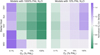 |
Fig. 3 Total O3 abundances for models with high N2O (left) and low N2O (right) normalized to models with modern levels of N2O from Kozakis et al. (2022). Overall, the high N2O models impacted the O2-O3 relationship more than the low N2O models, with the results being highly dependent on the stellar host and the amount of O2. High N2O models with hotter stars experience significant O3 depletion due to faster NOx catalytic cycles caused by increased N2O. However, for the high N2O models at very low O2 levels, planets around all the hosts experience an increase in O3 due to the higher efficiency of the smog mechanism once the Chapman mechanism is limited by low amounts of O2. The M5V-hosted planet in particular experiences an increase in O3 with the high N2O models beginning at 10% PAL O2 and lower, due to the increased capabilities of the smog mechanism in this lower UV environment. |
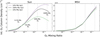 |
Fig. 4 O2-O3 relationship with high, low, and modern N2O models for planets around the Sun and M5V hosts. Vertical dashed lines indicate O2 levels of 100%, 10%, 1%, and 0.1% PAL. The phenomena causing maximum O3 production for the planet around the Sun to occur at O2 values less than the maximum O2 value modeled are explained in depth in Kozakis et al. (2022). In general, the M5V-hosted planet experiences significantly less variation in O3 for different N2O abundances than the Sun-hosted planet because the low UV flux of the M5V host is not as efficient at converting N2O into NOx as other hosts with higher UV fluxes. O2-O3 relationships for planets around all hosts and comparisons to Kozakis et al. (2022) are in Figure A.1. |
4.1.3 Atmospheric chemistry. Smog mechanism efficiency and NOx-limited and -saturated regimes
When varying the abundance of N2O – and therefore NOx – the smog mechanism of O3 production becomes particularly relevant. Described in Sect. 2.1, the smog mechanism uses NOx and HOx as catalysts to produce O3 in the lower atmosphere. This mechanism sources O atoms for O3 formation from NO2 photolysis, rather than O2 photolysis as with the Chapman mechanism. The ability for NO2 to be photolyzed by photons spanning the NUV and into the visible spectrum is in stark contrast to 242 nm required for O2 photolysis (see Fig. 2). Compared to the Chapman mechanism the smog mechanism can take place much deeper in the atmosphere and without the strong dependence on the host stars’ NUV flux. Although smog O3 production is increased for all high N2O cases, for the G0V-K5V hosted planets with O2 levels of ∼1% PAL and higher the destruction of O3 via the NOx catalytic cycle outweighs the extra smog-produced O3 in the troposphere. However, at 0.1% PAL O2 all cases with high N2O models show an increase in overall O3 abundance when compared to models with modern levels of N2O. This is because for low O2 levels the Chapman mechanism becomes severely limited by the amount of O2, while the smog mechanism is less impacted as it relies on NO2 photolysis instead. However, increased O3 smog production resulting in high O3 abundances is evident for the M5V-hosted planet at much higher O2 levels than other hosts, starting at 10% PAL O2.
There are two main reasons why the M5V-hosted planets experience a much stronger increase in smog mechanism O3 compared to other hosts:
the smog mechanism is much more accessible than the Chapman mechanism with lower incoming UV, as it is easier for the flux of the M5V host to photolyze NO2 rather than O2
only planets hosted by the M5V star never enter the NOx-saturated regime, meaning that the smog mechanism is not suppressed
This concept of NOx regimes (discussed in Sect. 2.2 and demonstrated in Fig. 1) is well-illustrated in Fig. 5, in which NO and HO2 mixing ratios for the Sun- and M5V-hosted planets are compared. Significant depletion of HO2 is observed in parts of the atmosphere existing in the NOx-saturated regime for the planet around the Sun. In the NOx-limited regime, increasing NOx allows the smog mechanism to create more O3, and O3 in turn creates O(1D) radicals that create HOx. However, when NOx levels are high enough to be in the NOx-saturated regime NOx is efficient at removing HOx by locking it up in reservoir species (such as HNO3 and HO2NO2), so an increase in NOx leads to a decrease in HOx. As hotter stars are more efficient at converting N2O into NOx – with the highest efficiency at high O2 – NO levels become high enough to enter the NOx-saturated regime and significantly reduce the effectiveness of the smog mechanism. For G0V-K2V hosted-planets with 100% PAL O2 all levels of N2O explored in this study sustain high enough NO mixing ratios in parts of the lower atmosphere to be in the NOx-saturated regime. At modern and high N2O levels parts of the atmosphere also enter the NOx-saturated regime for the G0V-, Sun-, and K2V-hosted planets at 10% PAL O2, as well the G0V and Sun cases slightly at 1% PAL O2. On the other hand, the low UV flux of the M5V host star struggles to convert N2O into NOx, consistently keeping it in the NOx-limited regime and allowing for a boost in smog O3 production whenever N2O is increased.
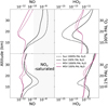 |
Fig. 5 NO and HO2 profiles at 100 and 0.1% PAL O2 for planets around the Sun and M5V hosts. Plots containing NO profiles indicate the NOx-saturated regime by a gray background, while the NOx-limited regime has a white background. When NO profiles enter the NOx-saturated regime, a corresponding depletion of HO2 appears in the same part of the atmosphere. The Sun-hosted planet often enters the NOx-saturated regime, due to the efficient conversion of N2O into NOx. By contrast, the M5V-hosted planet is less efficient at creating NOx in its low UV environment and remains in the NOx-limited regime. |
4.2 UV to ground
This section explores how the changes in the O2-O3 relationship translate to changes in the surface UV environment when varying N2O. On modern Earth both O2 and O3 are very important for UV shielding, which is important for surface life to flourish. Although O2 is not as efficient at shielding UV as O3 (see a comparison of absorption cross sections in Fig. 2), it is significantly more abundant than O3, and thus being a large constituent of our atmosphere it provides significant shielding. We discuss surface UV environments using three biological regimes of UV: UVA (315–400 nm) is least damaging and may help power complex processes necessary for life; UVB (280–315 nm), which is more dangerous and has been linked to tanning of skin as well as skin cancer; and UVC (121.6–280 nm), which is dangerous for biological organisms and can break apart DNA. On modern Earth UVA is not largely shielded by O3 or O2, UVB is partially shielded by O3, and fortunately UVC is almost entirely shielded by O2 and O3, protecting surface life. UVB and particularly UVC have a nonlinear relationship with the amount of O2/O3, and are very sensitive to changes in O3. See Kozakis et al. (2022) for an in-depth description of the impacts of UV on the ground while varying only O2. Comparisons of the top-of-the-atmosphere (TOA) and integrated UVC surface flux (the most variable results) are shown in Fig. 6, with an additional table in the appendix (Table A.1) displaying absolute and normalized UVB and UVC surface fluxes. UVA results were unaffected when changing N2O, with all models allowing ∼80% of incoming UVA to reach the surface, as in Kozakis et al. (2022). This is unsurprising as O3 does not provide shielding at these wavelengths, with other species causing minimal absorption.
UVB surface flux displays more variation when changing levels of N2O, but always within an order of magnitude. Higher O2 levels allow larger variations in UVB surface fluxes, as there are typically higher O3 levels, resulting in greater absolute changes in O3 abundance and UV shielding ability. The high N2O models showed the largest change in surface UVB flux at high O2 levels as increased efficiency of the NOx catalytic cycle caused significant changes in O3 for planets around all hosts except for the M5V. The most variation was at 100% PAL O2 for the G0V-hosted planet with 1.8 times as much UVB flux reaching the surface for the high N2O models, and 0.72 times as much flux reaching the surface for low N2O models. The only planet not experiencing large changes in UVB surface flux at these O2 levels for varying N2O cases was the one hosted by the M5V star, as the low UV flux did not allow efficient conversion of N2O into NOx, and did not impact O3 abundance as much as other hosts.
The most significant changes in the UV surface environment were for the UVC surface flux as it covers the wavelength range in which O3 shielding is most effective, causing O3 changes from varying N2O to strongly impact UVC surface flux. Similarly to UVB surface flux, for all but the planet hosted by the M5V star, the largest changes in UVC surface flux were caused by the high N2O cases at higher O2 levels. This was due once again to the significantly increased efficiency of the NOx catalytic cycle with increased NOx sourced from N2O. The largest increase was observed for the G0V-hosted planet with the high N2O model at 100% PAL O2, which experienced an astounding 15 billion-fold increase in UVC surface flux. However, even with this extreme increase in surface UVC flux this case still experiences less surface UVC flux than planets around all other hosts except the M5V for the high N2O models at this O2 level. This is because initially the G0V-hosted planet had the strongest UVC shielding at 100% PAL O2 due to having the highest O3 abundance. The ability of the high N2O models to deplete O3 with sufficient O2 is still seen at the 10% PAL O2 level where there were still significant increases in surface UVC flux for planets around all hosts except for the M5V, which had less surface UVC due to increased amounts of smog produced O3 around hosts with lower UV. For our lowest O2 levels planets around all hosts start to show decreased levels of UVC surface flux for the high N2O models compared to modern levels of N2O due to the extra UV shielding from the O3 produced by the smog mechanism.
The largest reduction of UVC surface flux from the low N2O models was observed for the Sun-hosted planet, with a factor of 4.1 × 10⁻⁶ times the original UVC surface flux with modern N2O at 100% PAL O2, due to a less productive NOx catalytic cycle. From the high N2O models the largest UVC surface flux reduction was observed for the planet around the G0V host at 0.1% PAL O2, with only a factor of 0.19 UVC flux reaching the surface compared to modern N2O levels due to extra O3 from smog production. Overall the N2O models with the least UVC surface flux variation were those around the M5V host, due largely to the fact that these cases had the least amount of total O3, so the absolute amount of surface flux does not have much variation.
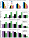 |
Fig. 6 UVC surface fluxes for planets around all hosts from Kozakis et al. (2022) with modern N2O (top) and with high and low N2O abundances from this study with O2 levels of 100% (second row), 10%, (third row), and 0.1% (bottom) PAL. The first panel in the top row indicates the top-of-the-atmosphere (TOA) flux for planets around all host stars, with the rest of the top row using the same y-axis limits for the corresponding O2 values used in the bottom three rows to facilitate comparisons. Results for 1% PAL O2 are extremely similar to those for 10% PAL O2 and are therefore not included. The most significant changes in UVC surface flux occur in models with higher O2 because the conversion from N2O to NOx is more efficient in higher O2 environments. Larger amounts of NOx have a greater impact on O3 either by depleting it with NOx catalytic cycles or producing it with the smog mechanism. While the results at 10% and 100% PAL O2 tend to show increased O3 shielding for low N2O models, this trend reverses at 0.1% PAL O2, where the low N2O models consistently receive more surface UVC. This is because at low O2 levels the effects of the smog mechanism become clearer as the Chapman mechanism is limited by the lack of O2. |
4.3 Planetary emission spectra
In this section we examine how the effects of N2O on the O2-O3 relationship would impact potential future observations. We focus in particular on the 9.6 µm O3 feature to see how it would change for different N2O abundances. Already in Kozakis et al. (2022) we found that just varying levels of O2 results in counterintuitive changes in the depth of the O3 spectral feature. This is due to the fact that spectral feature depth for emission spectra is dependent on not only the abundance of O3, but also the temperature difference between the absorbing and emitting layers of the atmosphere. This causes a nonlinear relationship between O3 abundance and feature depth as O3 has a significant impact on stratospheric heating. Ozone absorption features for planets with significant stratospheric heating will be shallower due to a decreased temperature difference between the stratosphere and surface when compared to a planet with less O3 and less stratospheric heating. This effect impacts planets around hotter stars more than those around cooler stars, as O3 heats the atmosphere via absorption of NUV photons and cooler stars (especially M dwarfs) have less NUV flux due lower temperatures and TiO absorption. Since the atmospheres of planets around cooler stars tend to be more isothermal, spectral feature depth has a more linear relationship between O3 abundance and O3 feature depth, as seen in the left-hand side of Fig. 7, which displays emission spectra from Kozakis et al. (2022). For a more in-depth look at how this effect impacts O3 spectral features with varying O2 levels please refer to Kozakis et al. (2022).
Figure 7 shows 9.6 µm O3 features with varying N2O normalized to features with modern levels of N2O in order to understand how observations of O3 could be impacted by varying N2O abundances. When comparing model atmospheres with varying N2O to those with modern levels of N2O, the largest changes in temperature profiles (and, therefore, the spectral features) were due to changing amounts of stratospheric heating from O3, which often was not a large change. As a result, changes in the O3 feature depth were due primarily to variations in O3 abundance, rather than the atmospheric temperature profile as in Kozakis et al. (2022). Overall the most significant changes in spectral feature strength were caused by the high N2O models at higher O2 levels, which is unsurprising as these are the cases with the largest depletion in O3 from the enhanced NOx catalytic cycle. The planet around the K2V host at 100% PAL O2 with the high N2O model has the spectral feature that changes the most compared to modern levels of N2O, with a shallower feature caused by O3 depletion. At 0.1% PAL O2 for planets around all hosts there is a deeper O3 feature due to the extra O3 produced by the smog mechanism at low levels of O2. There is less variation in spectral feature strength for the low N2O models as they had a much weaker effect on O3.
5 Discussion
5.1 Comparisons to other studies
Here we discuss studies examining how changes in N2O would impact a planet, especially with different O2 and O3 levels. For a full review of studies exploring the relationship between O2 and O3, see Kozakis et al. (2022). While no other study varied N2O specifically to look at changes in the O2-O3 relationship, there exist studies similar enough that it is useful to compare trends.
Grenfell et al. (2006) explores the possibility that on early Earth during periods with low O2, O3 produced by the smog mechanism using NO2 photolysis instead of O2 photolysis could have provided UV shielding for surface life. Motivated by the fact that HOx levels and possibly N2O levels were higher during the Proterozoic period (2.4–0.54 Gyr ago), they varied CH4, O2, NOx, H2, and CO abundances to study the impact on smog O3 formation using a photochemistry box model. Although they explore a different parameter space than in this study, similar trends appear, and they also see the effects of the atmosphere in a NOx-saturated regime, which suppresses O3 formation, similarly to what we find at high N2O in our model atmospheres around the hotter stars.
There are also several studies in a similar vein focusing on planets in M dwarf systems, especially since the low incoming UV from such hosts could lead to a buildup of N2O in their atmospheres (Segura et al. 2003, 2005). Rauer et al. (2011) and Grenfell et al. (2013) – both part of the same paper series – discuss the increased smog production efficiency of planets around M dwarfs, particularly late-type M dwarfs. This idea is explored in depth in Grenfell et al. (2013), where they use the Pathway Analysis Program (Lehmann 2004) to compare the efficiencies of the Chapman and smog mechanisms of O3 production. Although they use an earlier version of Atmos for their atmospheric modeling, they utilize a more complex chemical network to study smog formation, including variations of the smog mechanism that are not included in our chemical network that involve more complex methyl-containing molecules (e.g., CH3O2). However, the “classical” smog mechanism that we use in this study is shown to be the most common type of smog production. The trends reported in Grenfell et al. (2013) agree with those discussed in this study, especially with our results for increased smog production of O3 around our coolest host, the M5V. However, Grenfell et al. (2013) do not vary O2 or N2O abundances. Another study, Grenfell et al. (2014), varies N2O and CH4 biological surface fluxes, along with incoming UV fluxes to explore the effect of a planet orbiting an M7V host star. Although they use an M7V host star and explore different N2O abundances than in this paper (N2O at a factor of 1000 lower and zero N2O flux), similar trends are observed – particularly decreased smog production for decreased N2O, which we see especially in our models around cooler host stars.
Schwieterman et al. (2022) explores what a plausible range of N2O surface fluxes could be for terrestrial planets using both a biogeochemical model and a photochemistry model (from Atmos). Using the biogeochemical model cGENIE they predict possible N2O surface fluxes based off denitrification process at O2 abundances from 1–100% PAL with planet hosts ranging from F2V to M8V. By modeling total ocean denitrification they determine maximum N2O atmospheric mixing ratios for different O2 abundances. Their results show that our high N2O models (using an N2O mixing ratio of 3 ppm) are safely within the range of possible N2O values for all spectral host types. Although Schwieterman et al. (2022) also explores atmospheres with different amounts of N2O and O2 as in our study, the focus is not on O3 so it is difficult to make direct comparisons. Schwieterman et al. (2022) briefly show that increasing N2O results in increased destruction of stratospheric O3, agreeing with our general results, although they do not discuss if increased smog mechanism formation occurs at large N2O values. Overall, when comparing our current study to other similar works there appears to be no real inconsistencies, although the studied parameter spaces are varied enough that it is not possible to make direct comparisons.
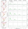 |
Fig. 7 9.6 µm O3 feature for models from Kozakis et al. (2022) (left) and normalized models from varying N2O (right) from simulated planetary emission spectra. Changes in the O3 feature for this study depended primarily on changes in O3 abundance – rather than on changes in the atmospheric temperature profile, as in Kozakis et al. (2022) – since varying N2O often did not significantly impact the temperature profiles. As the K5V-hosted planet experienced the greatest change in O3 abundance with the high N2O models, it follows that its O3 emission spectral features were the most impacted. The M5V-hosted planet experienced the smallest change in O3 while varying N2O, which is reflected by the small variations in its O3 feature. |
5.2 Plausible N2O mixing ratios in Earth-like atmospheres
In this study we used fixed mixing ratio profiles for N2O to facilitate comparisons of how those levels of N2O were expected to impact the O2-O3 relationship across different host stars. However, it is important to recognize that the relationship between surface flux and resulting atmospheric mixing ratios is not linear, and is highly influenced by the host star as well as atmospheric content. For N2O in particular the O2 level has significant impact on the resulting mixing ratio, meaning that there would be a range of N2O fluxes that would be necessary to reproduce the mixing ratios used in this study. As stated in Sect. 3, the motivation behind our chosen N2O abundances is to begin filling in the parameter space of how atmospheric variations impact the O2-O3 relationship. Using such a large range of N2O allows us to understand in which scenarios we would expect O3 abundances to be impacted in a way that would make observations more difficult to interpret. We briefly review expected N2O surface fluxes over time, and atmospheric parameters impact their mixing ratios.
As alluded to earlier, abundances of N2O can be strongly impacted by O2 abundances due primarily to UV shielding and reactions with O2 and oxygen-containing species. In addition, the level to which N2O can buildup in an atmosphere is also dependent on the host star, with cooler stars allowing for more buildup in their atmospheres due to lower incoming UV fluxes (e.g., Segura et al. 2003, 2005). As mentioned during the previous subsection, with N2O there has been work done to evaluate the maximum possible surface fluxes and corresponding mixing ratios using biogeochemical and photochemistry models (Schwieterman et al. 2022). It is also more complicated to evaluate these limits, since O2 influences both the surface flux and mixing ratio of N2O. The production of N2O surface flux is caused by nitrification and denitrification processes, whereas N2O mixing ratios depend on N2O destruction rates via photolysis and O(1D) radicals in the stratosphere. For both surface flux and atmospheric mixing ratios, the dependence on O2 is complicated, as nitrification processes require O2 and denitrification processes require an absence of O2. Moreover, while O2 also creates O3, which protects atmospheric N2O from photolysis, increased O2 also causes increased O(1D) radicals – another major sink for N2O. Additionally, due to the dependency on incoming UV, the amount of N2O in the atmosphere is highly influenced by the host star, requiring careful modeling.
It is possible that N2O surface fluxes were much higher in the past, particularly during the Proterozoic era. On modern Earth the majority of denitrification processes end with N2O being converted into N2, but this conversion requires a metal catalyst, most commonly Copper (see Schwieterman et al. 2022 for details). However during the Proterozoic era it is estimated that the oceans were highly depleted of Copper (Saito et al. 2003; Zerkle et al. 2006; Roberson et al. 2011), potentially causing significantly higher N2O fluxes as N2O would not be converted into N2. Although, for planets around hotter stars like the Sun in order not to have widespread depletion of N2O via photolysis, O2 levels of about 10% PAL would be necessary to provide UV shielding (Roberson et al. 2011). If so, N2O could have accumulated on Proterozoic Earth to levels high enough to contribute to warming during this time period.
6 Summary and conclusions
This study focuses on how varying N2O abundances in the atmosphere of an Earth-like planet impact the O2-O3 relationship across a range of O2 levels around a variety of host stars. We find that the impact of varying N2O depends on both the host star and the amount of O2 in the atmosphere (see Fig. 3). Adding additional N2O to an atmosphere rather than removing it consistently yielded more significant changes to O3 formation and destruction.
Atmospheric chemistry for models with varying N2O (Sect. 4.1) show that, for O2 levels greater than 1% PAL, planets around all hosts except the M5V experience significant depletion in O3 in the high N2O models compared to modern levels of N2O, due to the enhanced efficiency of the NOx catalytic cycle. Planets around the M5V hosts are the least impacted by this effect, due to their low-incoming UV flux having a weakened ability to convert N2O into NOx. However, the M5V-hosted planets were most efficient at creating extra O3 at high N2O with the smog mechanism in the lower atmosphere, especially at lower O2 levels as the low UV environment was more suited to NO2 photolysis than O2 photolysis. At O2 levels of 0.1% PAL and lower, planets around all hosts experienced an increase in O3 with the high N2O models. This was due to the more dominant effects of the smog mechanism, as the Chapman mechanism was extremely limited by low O2. However, the increase was not as pronounced as that seen for the planet around the M5V host. This is because the higher efficiency of hotter stars in converting N2O into NOx resulted in NOx abundances high enough to reach the NOx-saturated regime, thereby suppressing O3 smog formation.
The UV flux reaching the surface of our model planets was impacted by the changes in O3 (Sect. 4.2) especially since O3 abundance and attenuation of UV in the atmosphere have a non-linear relationship. Results for the UVC surface flux are shown in Fig. 6, as this wavelength range is not only the most dangerous for life, but also the most sensitive to changes in O3. The most extreme example of changing UVC surface flux was observed for the G0V-hosted planet at modern levels of O2 and high N2O, which received a 15 billion-fold increase in UVC ground flux compared to modern levels of N2O. For planets around all the hosts except the M5V, the largest changes in UVC at the surface occurred in the high N2O cases. More flux reached the surface at O2 levels above 0.1% PAL due to NOx destroying O3, while less UV reached the ground in low O2 cases of 0.1% PAL because of additional UV shielding from O3 produced by the smog mechanism. However, for the high N2O models around the M5V host, there was greater UV shielding at O2 levels of 10% PAL and below, due to the increased O3 formed by the smog mechanism.
Lastly, we explored how changing N2O abundances could potentially impact O3 measurements in future observations and the ability to use O3 to learn about the amount of O2 in a planetary atmosphere (Sect. 4.3). We focused particularly on the 9.6 µm O3 feature for the simulated planetary emission spectra and how the feature would change with different abundances of N2O (Fig. 7). Unlike in Kozakis et al. (2022), changes in feature depth were influenced more by changes in O3 than by temperature profiles. While decreasing the amount of N2O had little impact on the O3 feature, increasing it had a significantly larger impact. The destruction of O3 for hotter hosts at high O2 levels particularly influenced the feature depth, resulting in shallower features, with the K5V-hosted planet being the most impacted. The planet around the M5V dwarf only had significant changes in the O3 feature for the high N2O models at low O2 levels, due to the amount of extra O3 produced by the smog mechanism in the lower atmosphere.
When considering this work in the context of planning future observations, no host star displayed results showing that O3 measurements in the mid-IR would be unaffected by the abundance of N2O in their atmospheres. We propose that a separate measurement of N2O is important for using O3 to assess the abundance of O2 in an atmosphere. Fortunately, if we consider mid-IR measurements once again, there exists a N2O feature, albeit overlapping with a CH4 feature, potentially causing data interpretation issues. A variety of studies have been carried out in preparation for future observations of the proposed LIFE mission in the mid-IR (e.g., Konrad et al. 2022; Alei et al. 2022; Konrad et al. 2023; Alei et al. 2024; Angerhausen et al. 2024); however, more in-depth studies focusing on the different levels of N2O would be helpful in the pursuit of using O3 as a means to learn about potential life on a terrestrial exoplanet.
Studying the O2-O3 relationship in the context of varying N2O abundances reveals another layer of complexity in addition to what we already find in Kozakis et al. (2022). As with all atmospheric measurements of terrestrial exoplanets, context will be essential for truly understanding the meaning of our observations. This work further reinforced the idea that understanding the host star is necessary to understand the planet. It also high-lights the need to measure additional atmospheric species before using O3 as a way to infer biologically produced O2 and the potential for surface life on a planet.
Acknowledgements
All computing was performed on the HPC cluster at the Technical University of Denmark (DTU Computing Center 2021). This project is funded by VILLUM FONDEN. Authors TK and LML acknowledge financial support from the Severo Ochoa grant CEX2021-001131-S funded by MCIN/AEI/10.13039/501100011033. JMM acknowledges support from the Horizon Europe Guarantee Fund, grant EP/Z00330X/1. We thank the anonymous referee for providing comments, which improved the clarity of our manuscript.
References
- Alei, E., Konrad, B. S., Angerhausen, D., et al. 2022, A&A, 665, A106 [NASA ADS] [CrossRef] [EDP Sciences] [Google Scholar]
- Alei, E., Quanz, S. P., Konrad, B. S., et al. 2024, A&A, 689, A245 [NASA ADS] [CrossRef] [EDP Sciences] [Google Scholar]
- Angerhausen, D., Pidhorodetska, D., Leung, M., et al. 2024, AJ, 167, 128 [NASA ADS] [CrossRef] [Google Scholar]
- Arney, G., Domagal-Goldman, S. D., Meadows, V. S., et al. 2016, Astrobiology, 16, 873 [Google Scholar]
- Batalha, N. E., Marley, M. S., Lewis, N. K., & Fortney, J. J. 2019, ApJ, 878, 70 [NASA ADS] [CrossRef] [Google Scholar]
- Batalha, N., Rooney, C., & MacDonald, R. 2021, https://doi.org/10.5281/zenodo.5093710 [Google Scholar]
- Braam, M., Palmer, P. I., Decin, L., et al. 2022, MNRAS, 517, 2383 [NASA ADS] [CrossRef] [Google Scholar]
- Chapman, S. A. 1930, Mem. R. Met. Soc., 3, 103 [Google Scholar]
- Des Marais, D. J., Harwit, M. O., Jucks, K. W., et al. 2002, Astrobiology, 2, 153 [NASA ADS] [CrossRef] [Google Scholar]
- DTU Computing Center 2021, DTU Computing Center resources [Google Scholar]
- Fauchez, T. J., Villanueva, G. L., Schwieterman, E. W., et al. 2020, Nat. Astron., 4, 372 [NASA ADS] [CrossRef] [Google Scholar]
- France, K., Loyd, R. O. P., Youngblood, A., et al. 2016, ApJ, 820, 89 [NASA ADS] [CrossRef] [Google Scholar]
- Gregory, B. S., Claire, M. W., & Rugheimer, S. 2021, Earth Planet. Sci. Lett., 561, 116818 [CrossRef] [Google Scholar]
- Grenfell, J. L., Stracke, B., Patzer, B., Titz, R., & Rauer, H. 2006, Int. J. Astrobiol., 5, 295 [NASA ADS] [CrossRef] [Google Scholar]
- Grenfell, J. L., Gebauer, S., Godolt, M., et al. 2013, Astrobiology, 13, 415 [CrossRef] [Google Scholar]
- Grenfell, J. L., Gebauer, S., v Paris, P., Godolt, M., & Rauer, H. 2014, Planet. Space Sci., 98, 66 [CrossRef] [Google Scholar]
- Haagen-Smit, A. J. 1952, Ind. Eng. Chem., 44, 1342 [Google Scholar]
- Harman, C. E., Schwieterman, E. W., Schottelkotte, J. C., & Kasting, J. F. 2015, ApJ, 812, 137 [NASA ADS] [CrossRef] [Google Scholar]
- Kasting, J. F. 1979, PhD thesis, University of Michigan, United States [Google Scholar]
- Kasting, J. F., & Ackerman, T. P. 1986, Science, 234, 1383 [NASA ADS] [CrossRef] [Google Scholar]
- Kasting, J. F., Holland, H. D., & Pinto, J. P. 1985, J. Geophys. Res. 90, 10497 [NASA ADS] [CrossRef] [Google Scholar]
- Kitzmann, D., Patzer, A. B. C., von Paris, P., Godolt, M., & Rauer, H. 2011, A&A, 531, A62 [NASA ADS] [CrossRef] [EDP Sciences] [Google Scholar]
- Konrad, B. S., Alei, E., Quanz, S. P., et al. 2022, A&A, 664, A23 [NASA ADS] [CrossRef] [EDP Sciences] [Google Scholar]
- Konrad, B. S., Alei, E., Quanz, S. P., et al. 2023, A&A, 673, A94 [NASA ADS] [CrossRef] [EDP Sciences] [Google Scholar]
- Kopparapu, R. K., Ramirez, R., Kasting, J. F., et al. 2013, ApJ, 770, 82 [NASA ADS] [CrossRef] [Google Scholar]
- Kozakis, T., Mendonça, J. M., & Buchhave, L. A. 2022, A&A, 665, A156 [NASA ADS] [CrossRef] [EDP Sciences] [Google Scholar]
- Kump, L. 2008, Nature, 451, 277 [NASA ADS] [CrossRef] [Google Scholar]
- Kurucz, R. L. 1979, ApJS, 40, 1 [NASA ADS] [CrossRef] [Google Scholar]
- Lederberg, J. 1965, Nature, 207, 9 [NASA ADS] [CrossRef] [Google Scholar]
- Léger, A., Fontecave, M., Labeyrie, A., et al. 2011, Astrobiology, 11, 335 [CrossRef] [Google Scholar]
- Lehmann, R. 2004, J. Atmos. Chem., 47, 45 [Google Scholar]
- Lippincott, E. R., Eck, R. V., Dayhoff, M. O., & Sagan, C. 1967, ApJ, 147, 753 [NASA ADS] [CrossRef] [Google Scholar]
- Logan, J. A., Prather, M. J., Wofsy, S. C., & McElroy, M. B. 1981, J. Geophys. Res.: Oceans, 86, 7210 [Google Scholar]
- Lovelock, J. E. 1965, Nature, 207, 568 [NASA ADS] [CrossRef] [Google Scholar]
- Léger, A., Pirre, M., & Marceau, F. J. 1993, A&A, 277, 309 [Google Scholar]
- Meadows, V. S. 2017, Astrobiology, 17, 1022 [CrossRef] [Google Scholar]
- Meadows, V. S., Arney, G. N., Schwieterman, E. W., et al. 2018a, Astrobiology, 18, 133 [Google Scholar]
- Meadows, V. S., Reinhard, C. T., Arney, G. N., et al. 2018b, Astrobiology, 18, 630 [Google Scholar]
- Nicolet, M. 1975, Planet. Space Sci., 23, 637 [Google Scholar]
- Quanz, S. P., Absil, O., Benz, W., et al. 2022, Experimental Astronomy, 54, 1197 [Google Scholar]
- Ratner, M. I., & Walker, J. C. G. 1972, J. Atmos. Sci., 29, 803 [NASA ADS] [CrossRef] [Google Scholar]
- Rauer, H., Gebauer, S., Paris, P. V., et al. 2011, A&A, 529, A8 [NASA ADS] [CrossRef] [EDP Sciences] [Google Scholar]
- Roberson, A. L., Roadt, J., Halevy, I., & F., K. J. 2011, Geobiology, 9, 313 [Google Scholar]
- Rugheimer, S., Kaltenegger, L., Segura, A., Linsky, J., & Mohanty, S. 2015, ApJ, 809, 57 [Google Scholar]
- Saito, M. A., Sigman, D. M., & Morel, F. M. 2003, Inorg. Chim. Acta, 356, 308 [Google Scholar]
- Schwieterman, E. W., Kiang, N. Y., Parenteau, M. N., et al. 2018, Astrobiology, 18, 663 [CrossRef] [Google Scholar]
- Schwieterman, E. W., Olson, S. L., Pidhorodetska, D., et al. 2022, ApJ, 937, 109 [NASA ADS] [CrossRef] [Google Scholar]
- Segura, A., Krelove, K., Kasting, J. F., et al. 2003, Astrobiology, 3, 689 [NASA ADS] [CrossRef] [Google Scholar]
- Segura, A., Kasting, J. F., Meadows, V., et al. 2005, Astrobiology, 5, 706 [Google Scholar]
- Shumilov, O. I., Kasatkina, E. A., Turyansky, V. A., Kyro, E., & Kivi, R. 2003, Adv. Space Res., 31, 2157 [Google Scholar]
- Teal, D. J., Kempton, E. M. R., Bastelberger, S., Youngblood, A., & Arney, G. 2022, ApJ, 927, 90 [NASA ADS] [CrossRef] [Google Scholar]
- Toon, O. B., McKay, C. P., Ackerman, T. P., & Santhanam, K. 1989, J. Geophys.Res., 94, 16287 [Google Scholar]
- Tuck, A. F. 1976, Q. J. Roy. Meteorol. Soc., 102, 749 [Google Scholar]
- Zahnle, K., Claire, M. W., & Catling, D. 2006, Geobiology, 4, 271 [CrossRef] [Google Scholar]
- Zerkle, A. L., House, C. H., Cox, R. P., & Canfield, D. E. 2006, Geobiology, 4, 285 [Google Scholar]
Appendix A Supporting figures and tables
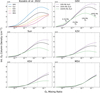 |
Fig. A.1 O2-O3 relationship for changing N2O, along with models from Kozakis et al. (2022) for comparison, for all modeled O2 mixing ratios. Vertical dashed lines indicate O2 levels of 100%, 10%, 1%, and 0.1% PAL. All plots share the same y-axis to facilitate comparison between different host stars. The phenomena that causes the peak O3 value for G0V-, Sun-, and K2V-hosted planets to occur at O2 levels less than the maximum value modeled (150% PAL O2) is discussed at length in Kozakis et al. (2022). |
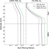 |
Fig. A.2 N2O profiles for planets around the Sun and M5V hosts at 100% and 1% PAL O2. The sun-hosted planet shows significant amounts of N2O depletion via photolysis (the main stratospheric sink of N2O), especially at lower O2 levels, as the UV protection from both O2 and O3 is significantly lessened. This depletion of N2O impacts the conversion of N2O to NOx. Meanwhile, the M5V-hosted planet experiences very little photolysis at all O2 levels, due to the low UV flux of the host star. |
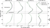 |
Fig. A.3 O3 profiles for varying N2O and O3 levels for planets around the Sun and the M5V hosts. The stratosphere (white background) and troposphere (gray background) are indicated in order to draw attention to differences in O3 production and depletion with the two stellar hosts. While at higher O2 levels the Sun-hosted planet efficiently destroys stratospheric O3, the M5V-hosted planet experiences minimal stratospheric O3 depletion at all O2 levels. The smog mechanism dominates in the lower atmosphere for the two hosts, especially at lower O2, but it is restricted to the troposphere for the planet around the Sun. Smog O3 is produced into the stratosphere for the planet around the M5V host, due to the lack of suppression the Sun-hosted planet experiences in the NOx-saturated regime. See Figs. 1 and 5 for more information on the NOx-limited and NOx-saturated regimes. |
UV Integrated Fluxes
All Tables
All Figures
|
Fig. 1 Impact of HO2 and OH in the NOx-limited and NOx-saturated regimes on modern Earth, adapted from Logan et al. (1981). In the NOx-limited regime (white background), increasing NOx allows for a more efficient smog mechanism, with the resulting increase in O3 causing a corresponding rise in HOx. In the NOx-saturated regime (gray background), the abundance of NOx rises to the point where smog O3 production is suppressed as NOx depletes HOx (a necessary catalyst for the smog mechanism) by locking it up into reservoir species. |
| In the text | |
|
Fig. 2 UV stellar spectra of the host stars in this study (top) and corresponding absorption cross sections of relevant gaseous species (bottom). The two plots cover the same wavelength range in order to facilitate comparisons. Cross sections for NO2 and N2O are cut off at shorter wavelengths, due to the dominance of absorption from CO2 and other atmospheric species. |
| In the text | |
|
Fig. 3 Total O3 abundances for models with high N2O (left) and low N2O (right) normalized to models with modern levels of N2O from Kozakis et al. (2022). Overall, the high N2O models impacted the O2-O3 relationship more than the low N2O models, with the results being highly dependent on the stellar host and the amount of O2. High N2O models with hotter stars experience significant O3 depletion due to faster NOx catalytic cycles caused by increased N2O. However, for the high N2O models at very low O2 levels, planets around all the hosts experience an increase in O3 due to the higher efficiency of the smog mechanism once the Chapman mechanism is limited by low amounts of O2. The M5V-hosted planet in particular experiences an increase in O3 with the high N2O models beginning at 10% PAL O2 and lower, due to the increased capabilities of the smog mechanism in this lower UV environment. |
| In the text | |
|
Fig. 4 O2-O3 relationship with high, low, and modern N2O models for planets around the Sun and M5V hosts. Vertical dashed lines indicate O2 levels of 100%, 10%, 1%, and 0.1% PAL. The phenomena causing maximum O3 production for the planet around the Sun to occur at O2 values less than the maximum O2 value modeled are explained in depth in Kozakis et al. (2022). In general, the M5V-hosted planet experiences significantly less variation in O3 for different N2O abundances than the Sun-hosted planet because the low UV flux of the M5V host is not as efficient at converting N2O into NOx as other hosts with higher UV fluxes. O2-O3 relationships for planets around all hosts and comparisons to Kozakis et al. (2022) are in Figure A.1. |
| In the text | |
|
Fig. 5 NO and HO2 profiles at 100 and 0.1% PAL O2 for planets around the Sun and M5V hosts. Plots containing NO profiles indicate the NOx-saturated regime by a gray background, while the NOx-limited regime has a white background. When NO profiles enter the NOx-saturated regime, a corresponding depletion of HO2 appears in the same part of the atmosphere. The Sun-hosted planet often enters the NOx-saturated regime, due to the efficient conversion of N2O into NOx. By contrast, the M5V-hosted planet is less efficient at creating NOx in its low UV environment and remains in the NOx-limited regime. |
| In the text | |
|
Fig. 6 UVC surface fluxes for planets around all hosts from Kozakis et al. (2022) with modern N2O (top) and with high and low N2O abundances from this study with O2 levels of 100% (second row), 10%, (third row), and 0.1% (bottom) PAL. The first panel in the top row indicates the top-of-the-atmosphere (TOA) flux for planets around all host stars, with the rest of the top row using the same y-axis limits for the corresponding O2 values used in the bottom three rows to facilitate comparisons. Results for 1% PAL O2 are extremely similar to those for 10% PAL O2 and are therefore not included. The most significant changes in UVC surface flux occur in models with higher O2 because the conversion from N2O to NOx is more efficient in higher O2 environments. Larger amounts of NOx have a greater impact on O3 either by depleting it with NOx catalytic cycles or producing it with the smog mechanism. While the results at 10% and 100% PAL O2 tend to show increased O3 shielding for low N2O models, this trend reverses at 0.1% PAL O2, where the low N2O models consistently receive more surface UVC. This is because at low O2 levels the effects of the smog mechanism become clearer as the Chapman mechanism is limited by the lack of O2. |
| In the text | |
|
Fig. 7 9.6 µm O3 feature for models from Kozakis et al. (2022) (left) and normalized models from varying N2O (right) from simulated planetary emission spectra. Changes in the O3 feature for this study depended primarily on changes in O3 abundance – rather than on changes in the atmospheric temperature profile, as in Kozakis et al. (2022) – since varying N2O often did not significantly impact the temperature profiles. As the K5V-hosted planet experienced the greatest change in O3 abundance with the high N2O models, it follows that its O3 emission spectral features were the most impacted. The M5V-hosted planet experienced the smallest change in O3 while varying N2O, which is reflected by the small variations in its O3 feature. |
| In the text | |
|
Fig. A.1 O2-O3 relationship for changing N2O, along with models from Kozakis et al. (2022) for comparison, for all modeled O2 mixing ratios. Vertical dashed lines indicate O2 levels of 100%, 10%, 1%, and 0.1% PAL. All plots share the same y-axis to facilitate comparison between different host stars. The phenomena that causes the peak O3 value for G0V-, Sun-, and K2V-hosted planets to occur at O2 levels less than the maximum value modeled (150% PAL O2) is discussed at length in Kozakis et al. (2022). |
| In the text | |
|
Fig. A.2 N2O profiles for planets around the Sun and M5V hosts at 100% and 1% PAL O2. The sun-hosted planet shows significant amounts of N2O depletion via photolysis (the main stratospheric sink of N2O), especially at lower O2 levels, as the UV protection from both O2 and O3 is significantly lessened. This depletion of N2O impacts the conversion of N2O to NOx. Meanwhile, the M5V-hosted planet experiences very little photolysis at all O2 levels, due to the low UV flux of the host star. |
| In the text | |
|
Fig. A.3 O3 profiles for varying N2O and O3 levels for planets around the Sun and the M5V hosts. The stratosphere (white background) and troposphere (gray background) are indicated in order to draw attention to differences in O3 production and depletion with the two stellar hosts. While at higher O2 levels the Sun-hosted planet efficiently destroys stratospheric O3, the M5V-hosted planet experiences minimal stratospheric O3 depletion at all O2 levels. The smog mechanism dominates in the lower atmosphere for the two hosts, especially at lower O2, but it is restricted to the troposphere for the planet around the Sun. Smog O3 is produced into the stratosphere for the planet around the M5V host, due to the lack of suppression the Sun-hosted planet experiences in the NOx-saturated regime. See Figs. 1 and 5 for more information on the NOx-limited and NOx-saturated regimes. |
| In the text | |
Current usage metrics show cumulative count of Article Views (full-text article views including HTML views, PDF and ePub downloads, according to the available data) and Abstracts Views on Vision4Press platform.
Data correspond to usage on the plateform after 2015. The current usage metrics is available 48-96 hours after online publication and is updated daily on week days.
Initial download of the metrics may take a while.