| Issue |
A&A
Volume 665, September 2022
|
|
|---|---|---|
| Article Number | A156 | |
| Number of page(s) | 18 | |
| Section | Planets and planetary systems | |
| DOI | https://doi.org/10.1051/0004-6361/202244164 | |
| Published online | 27 September 2022 | |
Is ozone a reliable proxy for molecular oxygen?
I. The O2–O3 relationship for Earth-like atmospheres
National Space Institute, Technical University of Denmark,
Elektrovej,
2800
Kgs. Lyngby, Denmark
e-mail: This email address is being protected from spambots. You need JavaScript enabled to view it.
Received:
1
June
2022
Accepted:
7
August
2022
Abstract
Molecular oxygen (O2) paired with a reducing gas is regarded as a promising biosignature pair for the atmospheric characterization of terrestrial exoplanets. In circumstances when O2 may not be detectable in a planetary atmosphere (e.g., at mid-IR wavelengths) it has been suggested that ozone (O3), the photochemical product of O2, could be used as a proxy to infer the presence of O2. However, O3 production has a nonlinear dependence on O2 and is strongly influenced by the UV spectrum of the host star. To evaluate the reliability of O3 as a proxy for O2, we used Atmos, a 1D coupled climate and photochemistry code, to study the O2–O3 relationship for “Earth-like” habitable zone planets around a variety of stellar hosts (G0V-M5V) and O2 abundances. Overall, we found that the O2–O3 relationship differed significantly with stellar hosts and resulted in different trends for hotter stars (G0V-K2V) versus cooler stars (K5V-M5V). Planets orbiting hotter host stars counter-intuitively experience an increase in O3 when O2 levels are initially decreased from 100% Earth’s present atmospheric level (PAL), with a maximum O3 abundance occurring at 25–55% PAL O2. As O2 abundance initially decreases, larger amounts of UV photons capable of O2 photolysis reach the lower (denser) regions of the atmosphere where O3 production is more efficient, thus resulting in these increased O3 levels. This effect does not occur for cooler host stars (K5V-M5V), since the weaker incident UV flux does not allow O3 formation to occur at dense enough regions of the atmosphere where the faster O3 production can outweigh a smaller source of O2 from which to create O3. Thus, planets experiencing higher amounts of incident UV possessed larger stratospheric temperature inversions, leading to shallower O3 features in planetary emission spectra. Overall it will be extremely difficult (or impossible) to infer precise O2 levels from an O3 measurement, however, with information about the UV spectrum of the host star and context clues, O3 will provide valuable information about potential surface habitability of an exoplanet.
Key words: astrobiology / planets and satellites: terrestrial planets / planets and satellites: atmospheres
© T. Kozakis et al. 2022
 Open Access article, published by EDP Sciences, under the terms of the Creative Commons Attribution License (https://creativecommons.org/licenses/by/4.0), which permits unrestricted use, distribution, and reproduction in any medium, provided the original work is properly cited.
This article is published in open access under the Subscribe-to-Open model. This email address is being protected from spambots. You need JavaScript enabled to view it. to support open access publication.
1 Introduction
In the search for life in the Universe, molecular oxygen (O2) is commonly recognized as a promising atmospheric biosignature gas. However, while O2 is largely created by biological sources on Earth, it can also be produced abiotically in a variety of settings, and thus alone would not constitute a guarantee of life (e.g., Hu et al. 2012; Wordsworth & Pierrehumbert 2014; Domagal-Goldman et al. 2014; Tian et al. 2014; Luger & Barnes 2015; Gao et al. 2015; Harman et al. 2015). Instead of being a standalone biosignature, O2 as a biosignature will be most powerful when detected simultaneously with a reducing gas as a “disequilibrium biosignature pair” (e.g., Lovelock 1965; Lederberg 1965; Lippincott et al. 1967), and when evidence of abiotic O2 production scenarios can be ruled out (see Meadows 2017; Meadows et al. 2018b for a review).
In scenarios where O2 is not directly detectable, it has been suggested that its photochemical product ozone (O3) could be used as a proxy for O2 (e.g., Leger et al. 1993; Des Marais et al. 2002; Segura et al. 2003; Léger et al. 2011; Meadows et al. 2018b). Using O3 as a proxy for O2 would be extremely useful in two particular scenarios: 1) at wavelengths where O2 features are not present (i.e., mid-infrared wavelengths), and 2) when O2 is present in small amounts (as it was for a significant fraction of Earth’s geological history).
The mid-infrared wavelength region (MIR; 3–20 μm) provides an excellent opportunity for the search for life, as it contains features for multiple biosignature gases, as well for gaseous species that could provide evidence for or against biological O2 production (Des Marais et al. 2002; Schwieterman et al. 2018; Quanz et al. 2021). Furthermore, thermal emission observations are less impacted by clouds (e.g., Kitzmann et al. 2011), and could also allow measurements of a planet’s surface temperature (Des Marais et al. 2002). The collisionally-induced absorption O2 feature at 6.4 μm is the only MIR feature that allows for the direct detection of O2, although it would be extremely difficult to use for abundances of O2 consistent with biological production (Fauchez et al. 2020). It will, however, be useful for identifying high-O2 desiccated atmospheres, a possible mechanism for abiotic O2 production (Luger & Barnes 2015; Tian 2015). Inferring the presence of biologically produced O2 will be restricted to indirect detections via the 9.7 μm O3 feature in the MIR.
In addition, although O2 has existed in appreciable amounts on Earth for a significant part of its history, it has only existed in large amounts for a relatively short period of time, posing a fundamental drawback to O2 as a biosignature (Meadows et al. 2018b). Molecular oxygen was first created produced biologically ~2.7 Ga (billion years ago) by oxygenic photosynthesis via cyanobacteria, although it did not build up to appreciable amounts in Earth’s atmosphere until the Great Oxidation Event (GOE) ~2.45 Ga (see e.g., Catling & Kasting 2017 for a review). Although the Phanerozoic era (541 Ma-present day) saw the widespread colonization of land plants and O2 levels comparable to our present atmospheric level (PAL), during the Proterozoic era (2.5 Ga–541 Ma) it is expected O2 levels could have been significantly lower (Catling & Kasting 2017; Lenton & Daines 2017; Dahl & Arens 2020). As a result, it is likely that O2 only would have been detectable on Earth for the last ~0.5 Gyr. However, since O3 is a logarithmic tracer of O2, it is possible that O3 could be capable of revealing small, undetectable amounts of O2 (e.g., Kasting et al. 1985; Leger et al. 1993; Des Marais et al. 2002; Segura et al. 2003; Léger et al. 2011). Additionally, a detection of O3 could provide information about UV shielding, and whether surface life is adequately protected from high-energy UV capable of DNA damage.
Some studies have suggested or already adopted O3 as a substitute for O2 (e.g., Segura et al. 2003, Kaltenegger et al. 2020, Lin et al. 2021), and others have noted a potentially powerful “triple biosignature” in planetary emission with CO2, H2O, and O3, where O2 spectral features are absent (Selsis et al. 2002). O3 is also expected to build up in the stratospheres of planets, allowing characterization via transmission spectroscopy (e.g., Bétrémieux & Kaltenegger 2013, 2014; Misra et al. 2014; Meadows et al. 2018b).
However, it is uncertain how reliably a measurement of O3 could allow us to infer the amount of O2. Ozone is known to have a nonlinear relationship with O2, as well as a strong dependence on the UV spectrum of the host star (Ratner & Walker 1972; Kasting & Donahue 1980; Kasting etal. 1985; Segura etal. 2003; Rugheimer et al. 2013). Although several studies have modeled the O2–O3 relationship for varying O2 abundances and different stellar hosts (e.g., Ratner & Walker 1972; Levine et al. 1979; Kasting & Donahue 1980; Kasting etal. 1985; Segura etal. 2003; Gregory et al. 2021), there has been no in-depth study evaluating the ability of O3 to predict O2 as a biosignature. In this series of papers, we will explore the O2–O3 relationship in depth for a variety of stellar hosts and atmospheric conditions. For this first paper, we focus on the O2–O3 relationship for “Earth-like” planets for different stellar hosts. Here, we take Earth-like to mean a planet that has the same composition and size as Earth, receives the equivalent total incident flux from the Sun as modern Earth, and has a similar atmospheric composition. This study currently contains the largest number of models run with a fully coupled climate and photochemistry code dedicated to understanding the O2–O3 relationship, along with exploring the widest range of stellar hosts as well as the largest number of different O2 atmospheric abundances.
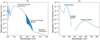 |
Fig. 1 Absorption cross sections of O2 (left) and O3 (right), both plotted on the same y-axis scale to enable easier comparison. The y-axis is the same for both to enable easier comparison. Relevant O2 bands are the Schumann-Runge continuum (137–175 nm), the Schuman-Runge bands (175–200nm), and the Herzberg continuum (195–242nm). For less than 175nm an excited O atom, the O(1D) radical, is formed along with a ground state O atom during photolysis. O3 bands are the Hartley bands (200–300 nm), the Huggins bands (310–350 nm), and the Chappuis bands (410–750 nm). Photolysis within the Hartley bands will produce the O(1D) radical while other O3 bands create a ground state O atom. Absorption cross section data is from Brasseur & Solomon (2005). |
2 Chemistry of O3 production and destruction
In this section, we give a brief overview of the most important reactions for the production and destruction of O3. The wavelength-dependent absorption cross sections for O2 and O3 are shown in Fig. 1 as a reference for the reader, as they determine photolysis rates in different wavelength regions. Incident stellar UV flux as well as the amount of nitrogen- and hydrogen-bearing species primarily control the concentration of O3 in the atmosphere.
2.1 The Chapman mechanism
Ozone is primarily created in the stratosphere by a set of reactions called the Chapman mechanism (Chapman 1930). These reactions begin with the photolysis of O2,
 (1)
(1)
which creates ground state O atoms (also written as O(3P)), which are highly reactive due to two unpaired electrons. These O atoms then combine with O2 molecules to form O3,
 (2)
(2)
where M is a background molecule that carries away excess energy. Reaction (2) is a 3-body reaction, meaning it is more efficient at lower temperatures and higher atmospheric densities. It is faster in denser atmospheric regions with a larger availability of O atoms, causing bulk of O3 on Earth to exist in the stratosphere rather than at higher altitudes.
Photolysis of O2 can also occur higher in the atmosphere with higher energy photons,
 (3)
(3)
where the O(1D) radical is created along with a ground state O atom. Free radicals are by nature extremely reactive as they have at least one unpaired valence electron. Thus, they tend to have extremely brief lifetimes. The O(1D) radical can return to the ground state by being “quenched” via a collision with a background molecule,
 (4)
(4)
or it can react with another molecule. Reactions with other molecules will be further explored in Sects. 2.2 and 4.1.
Although O2 absorption cross sections are significantly larger at wavelengths that produce O(1D) radicals (<175nm; see Fig. 1), these photons are absorbed high in the atmosphere and therefore do not contribute to the creation of stratospheric O3 on modern Earth. Absorption caused by Lyman-α photons (121.6 nm) is generally absorbed in the mesosphere, and photons in the Schumann-Runge continuum (130–175 nm) are absorbed in the thermosphere. Also note that some wavelengths shorter than Lyman-α can ionize O2, although that wavelength region is not included in our photochemistry model due to the low amount of photons in that region emitted by GKM stars (see Sect. 3.1).
Although O2 photolysis from these higher energy photons (<175 nm) occurs above the stratosphere on modern Earth, planets with different amounts of atmospheric O2 would experience absorption of these photons at varying atmospheric altitudes. Less O2 would allow high energy photons to travel deeper into the atmosphere before absorption via O2 photolysis. Although this will not cause the bulk of O3 formation, it will impact the upper atmospheric chemistry by creating more O(1D) at lower altitudes. The effects of this will discussed at length in Sect. 4.1.
Once O3 is created by Reaction (2), it is often quickly photolyzed. O3 photolysis from a photon in the Hartley band (200–300 nm) will create an O(1D) radical, while photons from the lower energy Huggins bands (310–350 nm), Chappuis bands (410–750 nm), and longer wavelengths will create a ground state O atom,
 (5)
(5)
 (6)
(6)
Photons with wavelengths shorter than 200 nm are often absorbed high in the atmosphere by O2 and other molecules. As with O2 photolysis, O(1 D) radicals created by Reaction (5) will either be quenched by a background molecule and returned to the ground state (Reaction (4)), or they will react with other molecules.
Photolysis of O3 is not seen as a loss of O3, as the resulting O atom and O2 molecule often quickly recombine into O3 via Reaction (2). Due to the rapid cycling between O3 and O, it is instead the conversion of O3 + O (called “odd oxygen”) into O2 that actually results in a loss of O3, as occurs in the final reaction of the Chapman mechanism,
 (7)
(7)
Odd oxygen (O3 + O) being converted into O2 is considered a loss of O3 because the photolysis of O2 (Reactions (1), (3)) is the slowest of the Chapman mechanism reactions, and the limiting factor in O3 production. Therefore the loss of odd oxygen on long timescales causes a true decrease in O3.
2.2 Catalytic cycles of HOx and NOx
The Chapman mechanism on its own overestimates the amount of atmospheric O3 because it does not take into account catalytic cycles that destroy O3. These destruction cycles follow the format,

where X is a free radical. During this process X and XO will cycle between each other while converting odd oxygen (O3 + O) into O2, similarly to the last step of the Chapman mechanism (Reaction (7)). As stated above, this results in the overall loss of O3 because O2 photolysis is the limiting reaction of O3 formation. X and XO can cycle between each other and continuously destroy O3 until reactions that convert either X or XO into non-reactive “reservoir” species occur. The primary catalytic cycles of O3 destruction in modern Earth’s atmosphere are the HOx (hydrogen oxide) and NOx (nitrogen oxide) catalytic cycles. We note that on modern Earth there are also O3 destroying catalytic cycles that are powered by molecular compounds primarily created anthropogenically (e.g., chlorine and bromine cycles; Crutzen & Lelieveld 2001), but they will not be included in this study.
The HOx catalytic cycle is powered by the OH (hydroxyl) and HO2 (hydroperoxyl) radicals. When an O(1D) radical is created either by photolysis of O2 (Reaction (3)) or O3 (Reaction (5)) it can react with H2O to form OH,
 (8)
(8)
The OH radical is a major sink for multiple atmospheric gases (e.g., CH4, CO) and is often called the ‘detergent of the atmosphere’ for this reason. It destroys O3 during the HOx catalytic cycle as follows,
 (9)
(9)
 (10)
(10)
In addition to this primary destruction cycle, other HOx cycles can contribute significantly to O3 destruction via,
 (9)
(9)
 (11)
(11)
resulting in two O3 molecules converted to three O2 molecules, or,
 (12)
(12)
 (13)
(13)
 (10)
(10)
with a net result of two O atoms converted into an O2 molecule. Because OH production via O(1D) is a byproduct of the Chapman mechanism, HOx catalytic cycle efficiency can be increased with higher rates of O3 formation. This process can be slowed through reactions that convert OH/HO2 into a reservoir species such as H2O, HNO2, or H2O2, which are significantly less reactive.
The NOx catalytic cycle destroys O3 with the NO (nitric oxide) and NO2 (nitrogen dioxide) radicals. The primary source of these radicals in the stratosphere is from N2O (nitrous oxide) which is biologically produced by nitrification and denitrification processes within soil. N2O can additionally be produced anthropogenically, primarily through agriculture. It is converted into NO by interactions with the O(1D) radical,
 (14)
(14)
A secondary source of NO is production via lightning in the upper troposphere, which can then be transported into the lower stratosphere. The NOx catalytic cycle destroys O3 as follows:
 (15)
(15)
 (16)
(16)
NOx can destroy O3 with the following cycle as well,
 (15)
(15)
 (17)
(17)
 (18)
(18)
with a net conversion of two O3 molecules into three O2 molecules. NOx reactions are highly temperature dependent and are faster at hotter temperatures. The main reservoir species associated with NOx are HNO3 and N2O5, which have slow photolysis rates.
We note that although in the stratosphere NOx destroys O3 through this catalytic cycle, that lower in the atmosphere it can help create O3 through the “smog mechanism” (see Sect. 5.2). This low altitude O3 is a pollutant that can cause biological damage. In this study we will focus on the majority of O3 in the stratosphere created by the Chapman mechanism. In this study we will focus on the efficiency of the Chapman mechanism, along with the ability of the HOx and NOx catalytic cycles to destroy O3 for varying O2 levels around different host stars.
3 Methods
3.1 Atmospheric models
We modeled planetary atmospheres with Atmos1, a 1D coupled climate and photochemistry code to explore O3 formation for varying levels of O2 on Earth-like planets around a variety of host stars. Numerous studies have used either of these climate or photochemistry modules, as well as both coupled (e.g., Arney et al. 2017; Meadows et al. 2018a; Lincowski et al. 2018; Madden & Kaltenegger 2020; Gregory et al. 2021; Teal et al. 2022). We give a brief overview of Atmos and refer readers to Arney et al. (2016) and Meadows et al. (2018a) for extensive details.
The photochemistry model originates from Kasting (1979) and was expanded upon and updated by Zahnle et al. (2006). It has been used extensively by many studies (e.g., Kasting & Donahue 1980; Segura et al. 2003, 2005, 2010; Domagal-Goldman et al. 2014; Gregory et al. 2021). The atmosphere is broken up in 200 plane parallel layers from 0 to 100 km. The abundance of each gaseous species is calculated simultaneously with the flux and continuity equations using a reverse-Euler method for individual atmospheric layers. Vertical transport between different layers include molecular and eddy diffusion. Radiative transfer is computed with a δ-2-stream method as described in Toon et al. (1989). For modern Earth Atmos uses 50 gaseous species, with nine of them being short lived and thus not included in transport calculations. The photochemistry model is considered converged when its adaptive time step length reaches 1017 s within 100 time steps.
The climate model was originally developed by Kasting & Ackerman (1986), but has been significantly updated as described in Kopparapu et al. (2013) and Arney et al. (2016). Multiple studies have used this code to calculate habitable zones around a variety of stellar hosts used to study habitable zones and atmospheres of Earth-like planets around different stars (e.g., Kopparapu et al. 2013; Segura et al. 2003, 2005, 2010). The atmosphere is broken up into 100 plane parallel layers from the surface to an atmospheric pressure of 1 mbar. A correlated-k method computes the absorption of O3, H2O, CH4, CO2, and C2H6 throughout the atmosphere. Total absorption of incident stellar flux is calculated for each atmospheric layer with a δ-2-stream scattering algorithm (Toon et al. 1989), and outgoing IR radiation is calculated with correlated-k coefficients for each species individually. Updated H2O cross sections from Ranjan et al. (2020) have been incorporated into the code. Convergence criteria are reached when both changes in temperature and the flux out of the top of the atmosphere are sufficiently small (<10−5).
We run the climate and photochemistry models coupled with inputs including host stellar spectrum (121.6–45 450 nm), initial mixing ratios of atmospheric species, upper and lower boundary conditions for individual species, and initial temperature/pressure profiles. Using initial conditions the photochemistry code runs first and then transfer computed H2O, CH4, CO2, and C2H6 mixing ratio profiles to the climate code. The climate code then updates the temperature and H2O vapor profiles to feed back into the photochemistry. These processes iterate with profiles from the photochemistry allowing for more accurate climate code calculations and vice-versa, until a converged solution is reached.
The climate code has not been successfully run to convergence for the same atmospheric height as the photochemistry code (Arney et al. 2016), so temperature and H2O profiles of the upper, thin part of the atmosphere (typically <60–70 km) are held constant at the highest computed value from the climate code. Sensitivity tests from Arney et al. (2016) suggest that the impact on the radiative transfer and climate of these models is not significant.
This study also implements the “short-stepping” method of convergence, as described in Teal et al. (2022). When iterating back and forth between the photochemistry and climate code, occasionally the code will oscillate between two different solutions. For example, if the photochemistry code computes a large quantity of O3, the climate code will respond with a large amount of atmospheric heating. However, due to the temperature sensitivity of O3 production (Reaction (2)), this hotter atmosphere will cause lower amounts of O3 on the subsequent photochemistry iteration. Using the “short-stepping” method we do not allow the climate code to fully adjust to the updated atmospheric profiles from the photochemistry on a single iteration, and instead reach convergence slowly by iterating back and forth between the climate and photochemistry codes until a stable solution is reached.
We modeled planetary atmospheres orbiting a variety of stellar hosts (see Sect. 3.2) at the Earth-equivalent distance with varying levels of O2. Here, we take Earth-equivalent distance to mean that the planet receives the same total amount of incident flux from their parent stars as modern Earth receives from the Sun. We set O2 as a constant mixing ratio for all cases, with values varying from 0.01-150% PAL O2 (mixing ratios of 2.1 × 10⁻³–0.315). Higher O2 levels are not explored because large O2 levels would unstable with biological compounds (Kump 2008). Lower O2 are not modeled because it is thought that O2 abundances from ~10−3% to ~1% PAL are not expected to be stable in an Earth-like atmosphere as calculated by Gregory et al. (2021) (details on these limits in Sect. 5.4).
Other initial conditions for the models were chosen to resemble modern Earth including atmospheric mixing ratios, planetary composition, and size. Atmos haze production was not used. All models were run at a zenith of 60° degrees (Lambertian average) and with cloudless skies. Fixed mixing ratios were used for CH4 (1.8×10⁻⁶), N2O (3.0×10⁻⁷), and CO2 (3.6×10⁻⁴). All other species used initial atmospheric profiles and boundary conditions as defined in Atmos’s modern Earth template, and surface pressure remained constant at 1 bar. We note that defining CH4 at a constant mixing ratio resembling modern Earth differs from several studies modeling “Earth-like” planets, which have adjusted CH4 mixing ratios to reflect the CH4 ground flux of modern Earth, resulting in much higher atmospheric CH4 mixing ratios (e.g., Rugheimer et al. 2015a; Wunderlich et al. 2019; Teal et al. 2022). We chose to maintain CH4 mixing ratio of modern Earth to better isolate the effects of different stellar hosts on the O2–O3 relationship. The impact of changing CH4 levels on O3 abundance is discussed further in Sect. 5.2.
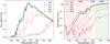 |
Fig. 2 Stellar spectra of the planet host stars. G0V-K5V hosts are comprised of IUE UV data from Rugheimer et al. (2013), and the M5V host comes from UV observations of GJ 876 from the MUSCLES survey (France et al. 2016). Visible and IR wavelengths use ATLAS models of the same stellar temperature (Kurucz 1979). The right-hand figure zooms in on the UV region relevant for photolysis with important biological UV regimes (see Sect. 4.4). |
3.2 Input stellar spectra
All host star spectra inputted into Atmos comprise of actual UV observations supplemented with synthetic ATLAS model spectra (Kurucz 1979) for the visible and IR. Table 1 contains information about the host stars and their spectra are shown in Fig. 2. The G0V-K5V stellar spectra were created in Rugheimer et al. (2013) and are a combination of UV data from the International Ultraviolet Explorer (IUE) data archives2 and model ATLAS spectra for the same stellar temperature (Kurucz 1979). UV data for the M5V host is from GJ 876 observations obtained by the Measurements of the Ultraviolet Spectral Characteristics of Low-mass Exoplanetary Systems (MUSCLES) survey (France et al. 2016).
The UV spectrum of a planet’s host star is extremely important in the photochemical modeling of O3 production. Not only does the total amount of UV dictate photolysis rates, but the UV spectral slope determines the creation and destruction rates of O3. The far-UV (FUV; λ < 200 nm) is primarily responsible for photolysis of O2 (and the creation of O3), while the mid- and near-UV (abbreviated NUV, for brevity; 200 nm < λ < 400 nm) is responsible for the photolysis of O3. The NUV additionally can photolyze H2O, which creates the HOx species responsible for destroying O3, causing NUV flux to destroy O3 both directly and indirectly. Hence, a higher FUV/NUV flux ratio will create O3 more efficiently. Low-mass, active stars tend to have lower FUV/NUV flux ratios as activity will cause excess FUV chromospheric radiation, while NUV wavelengths are often absorbed for cool stars by TiO (Harman et al. 2015).
Stellar hosts.
3.3 Radiative transfer model
After Atmos computes the compositions of our model atmospheres, the Planetary Intensity Code for Atmospheric Scattering Observations (PICASO) computes planetary emission spectra (Batalha et al. 2019, 2021). PICASO is a publicly available3 radiative transfer code capable of producing transmission, reflected light, and emission spectra for a diverse range of planets. Our emission spectra were calculated at a phase angle of 0° (full phase) with altitude dependent pressure, temperature and mixing ratio profiles computed by Atmos. Output spectra cover a wavelength range of 0.3–14 μm, although particular focus is put on the O3 9.7 μm feature in this study.
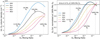 |
Fig. 3 O2–O3 relationship for Earth-like planets orbiting different host stars (indicated in legend) with varying amounts of O2 mixing ratios. Molecular oxygen levels compared to Earth’s present atmospheric level (PAL) are shown as dashed vertical lines for reference. The left-hand figure shows the relationship in terms of total integrated O3 column density, and the right-hand figure in terms of total O3 normalized at the amount produced in the 100% PAL O2 case for each stellar host. The nonlinearity in these relationships is primarily due to the pressure dependence of Reaction (2) which forms O3. The main takeaway is that the O2–O3 relationship is significantly different for hotter host stars (GOV, Sun, K2V) versus cooler host stars (K5V, M5V), with hotter hosts experiencing peak O3 formation occurring at O2 levels under 100% PAL. See Sect. 4.1 for a detailed explanation. |
4 Results
4.1 O2–O3 relationship
Figure 3 shows the O2–O3 relationship for all of our model planetary atmospheres. The O2–O3 relationship is highly dependent on the stellar host, with different trends for model atmospheres having hotter host stars (GOV, Sun, K2V) versus cooler host stars (K5V, M5V). Since O3 is produced via the Chapman mechanism by converting O2 into O3, one would naively expect the O3 concentration to increase as the O2 mixing ratio increases, which the case for the cooler host stars. However, the O2–O3 relationship for hotter stellar hosts behaves unexpectedly such that O3 abundance peaks and then decreases as the abundance of O2 decreases from modern Earth levels. Maximum O3 abundance occurs in the 25% PAL O2 models for the GOV and Sun hosts, and the 55% PAL O2 model for the K2V host. This effect does not occur for cooler host stars, with O3 abundance dropping consistently for models with less O2, though not in a linear fashion. As a result, the K5V and M5V models with maximum O2 considered (150% PAL) created the maximum amount of O3. These results are summarized in Table 2. To allow for a simple parameterization of the O2–O3 relationships shown in Fig. 3 that can be used as an approximation in, for instance, GCM and retrieval modeling, we fit a fifth degree polynomial of the form,
 (19)
(19)
where y is the integrated O3 column density (cm−2), x is the base 10 logarithm of the O2 mixing ratio, and α, b, c, d, e, and f are the best fit polynomial coefficients listed in Table 3. This fit is valid over the range of O2 abundances modeled in this study (0.01%–150% PAL).
The seemingly counterintuitive phenomenon of hotter hosts having O3 levels increase as O2 levels decrease can be explained by two factors: UV shielding abilities of O2, and the pressure dependency of O3 formation. First, we will address the UV shielding ability of O2. Despite the fact that O2 UV absorption cross sections are either significantly smaller than those of O3 or require far higher energy photons (see Fig. 1), O2 remains an important UV shield on modern Earth, primarily due to its large abundance. Although O2 is less efficient at absorbing UV photons than O3, O2 makes up ~21% of the atmosphere, whereas O3 is a trace gas with a maximum value of ~10 ppm on modern Earth. This allows the far larger number of O2 molecules to compensate for its smaller absorption crosssections and absorb many photons with wavelengths shorter than 240 nm (the required wavelength for O2 photolysis, see Reaction (1)). As a result, as O2 decreases, UV shielding in that wavelength range decreases, allowing photolysis to occur deeper in the atmosphere. This is illustrated in Fig. 4, where mixing ratio profiles of O3, H2O, CH4, and N2O are shown for all host stars at O2 abundances of 100%, 10%, 1%, and 0.1% PAL O2. Photolysis occurs at lower atmospheric altitudes as O2 decreases, leading the O3 layer to shift downward in the atmosphere. This effect is more pronounced for hotter host stars with high UV fluxes (particularly high FUV fluxes capable of O2 photolysis), and therefore higher photolysis rates.
Secondly, the depth in which O2 photolysis occurs is of particular importance to the altitudes at which the O3 forming Chapman mechanism takes place, because as O2 decreases, photolysis reaches not only deeper but also denser regions of the atmosphere. This is of significant relevance to O3 formation due to the pressure dependency of the Chapman mechanism: Reaction (2), in which an O atom and O2 molecule combine (with the help of a background molecule) to form O3, is a 3-body reaction, and therefore is faster at higher atmospheric densities. Denser regions allow O, O2, and background molecules to come together and react more rapidly than in a thinner region of the atmosphere. For hotter host stars in our sample (GOV, Sun, K2V), the UV fluxes are strong enough to allow O2 photolysis to reach much denser atmospheric layers as O2 decreases, allowing the benefit of faster O3 production via Reaction (2) to outweigh the smaller source of O2, resulting in peak O3 abundance at lower O2 levels.
Our cooler host stars (K5V, M5V), however, have weaker UV fluxes, meaning photons capable of O2 photolysis cannot travel as deep in the atmosphere as for hotter hosts when O2 decreases. The additional speed of the Chapman mechanism for lower O2 does not make up for the smaller amount of O2, causing O3 abundance to decrease for decreasing O2 abundance with these cooler host stars.
This result of an increase in O3 production as O2 levels decrease has been noted for the Earth-Sun system by several studies (e.g., Ratner & Walker 1972; Levine et al. 1979; Kasting & Donahue 1980; Kasting et al. 1985; Leger et al. 1993), although this is the first time it has been explored for Earth-like planets around different stellar hosts. Whether or not this would occur for an Earth-like planet will depend on if the UV flux (particularly the FUV flux) from its host star will be strong enough to incite O2 photolysis at dense enough atmospheric levels that the increased rate of O3 production will be enough to counter the decreased amounts of O2 from which O3 can form. This effect contributes to the strong dependency of the O2–O3 relationship on the spectral type of the host star. For example the G0V host star models have more O3 at 10% PAL O2 than at 100% PAL O2, whereas for the M5V host star O3 abundance in the 10% PAL O2 model is nearly 60% less than it is for the 100% PAL O2 model.
When looking at specific O3 mixing ratios, Fig. 3 also indicates an increase in O3 above the stratosphere for all models. This upper atmosphere O3 (the “secondary O3 layer”) is produced primarily by O2 photolysis from higher energy photons (>175nm; Reaction (3)) which produces the radical O(1D). Photons of these wavelengths are absorbed high in the atmosphere but do not contribute significantly to stratospheric O3, even when a decrease in O2 allows photolysis to reach deeper layers of the atmosphere. Instead, these photons create O3 above the primary O3 layer, generally in the mesosphere and thermosphere (see Sect. 2 for more details). Although O3 mixing ratios are high at these altitudes, due to the thin atmosphere, O3 creation at these elevations does not add considerably to the total amount of O3.
Also note that although the K2V host star produces enough UV photons capable of O2 photolysis to have peak O3 production in its 55% PAL O2 model, both the K5V and M5V host models show a larger amount of O3 than the K2V host for O2 levels near 100% PAL (Fig. 3). This is because although the K2V host has more FUV than the K5V and M5V hosts (Fig. 2), the cooler hosts have higher FUV/NUV ratios (Table 1), allowing more efficient O3 production without as much NUV O3 destruction.
In summary, the O2–O3 relationship is highly dependent on the UV flux of the host star, with different trends for hotter and cooler host stars. Hotter host stars with high FUV fluxes experience peak O3 abundance at lower O2 levels due to O3 formation occurring in deeper, denser parts of the atmosphere where the Chapman mechanism is more efficient. Cooler host stars do not emit enough FUV flux for this effect to occur, and experience consistently decreasing O3 as O2 decreases.
Maximum integrated O3 column density.
Coefficients of polynomial fit of the O2–O3 relationship.
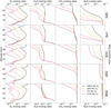 |
Fig. 4 Mixing ratio profiles of O3, H2O, CH4, and N2O; all potential biosignature species. Each row represents results for model atmospheres orbiting different stellar hosts as indicated on the right-hand vertical axis. Each plot shows the mixing ratio profiles for O2 abundances of 100%, 10%, 1% and 0.1% PAL. O2 on modern Earth is a significant UV shield, allowing model atmospheres with decreasing O2 values to have photolysis occur at consistently lower altitudes. This is demonstrated well with the bulk of O3 forming at lower altitudes with less O2, as well as increased upper atmospheric depletion for H2O, CH4, and N2O via photolysis. The downward shift of O3 and upper atmospheric depletion of other species is shown to decrease for model atmospheres around cooler stars with lower incident UV flux, and hence lower photolysis rates. Full details of this atmospheric chemistry is shown in Sects. 4.1 and 4.3. |
4.2 impact of varying O2 on H2O, CH4, and N2O
Figure 4 shows the impact of varying O2 levels on the biologically relevant atmospheres species H2O, CH4, and N2O. As O2 decreases, photons usually absorbed by O2 (λ < 240 nm) travel deeper into the atmosphere and drive the majority of atmospheric changes. This allows photolysis in general to reach lower altitudes, as well as photolysis caused by high energy photons that create the O(1D) radical, which reacts quickly with many species. O(1D) is produced via photolysis of O2, O3, N2O, and
CO2 as follows:
 (3)
(3)
 (5)
(5)
 (20)
(20)
 (21)
(21)
As O2 decreases, O(1 D) creation moves deeper into the atmosphere for all these species. For our models, O3 photolysis consistently creates the most O(1D), particularly at lower atmospheric heights. O2 photolysis is also a significant producer of O(1 D), although it is limited to the stratosphere and above, even for the lowest O2 levels modeled in this study. CO2 and N2O photolysis contribute to O(1D) production as well, although CO2 photolysis is constrained to the upper atmosphere similarly to O2 photolysis, while N2O photolysis can occur much closer to the planetary surface for low O2 levels. Increased rates of photolysis as O2 shielding decreases as well as increased O(1D) production reaching lower atmospheric levels causes the depletion of many species.
H2O is increasingly depleted for decreasing levels of O2 due to both photolysis in the atmosphere and O(1D) reactions lower in the atmosphere. Both of these reactions create the OH radical while removing H2O,
 (22)
(22)
 (8)
(8)
On modern Earth, Reaction (8) is the primary source of OH in the stratosphere, which is a major sink for several species. As H2O levels in the upper atmosphere drop with decreasing O2, this causes OH production to move to lower levels of the atmospheres as seen in Fig. 5. Upper atmospheric depletion of H2O and OH production at lower altitudes is seen more strongly for hotter host stars, as they have higher incident UV for photolysis and O(1D) creation.
CH4, an important biosignature gas, is also depleted in the upper atmosphere for models around all host stars, primarily though oxidation via OH (created via reactions with H2O), along with photolysis and reactions with O(1D),
 (23)
(23)
 (24)
(24)
In the upper atmosphere, depletion is dominated by photolysis. Reaction (23) is both the main sink of stratospheric CH4 and OH depletion on modern Earth, with CH4 and OH acting as a major sinks for each other. Reactions with O(1D) and OH occur deeper in the atmosphere for decreasing O2 levels as both these radicals are produced at lower altitudes. Reaction (24) is an additional source of OH in the lower stratosphere/troposphere. CH4 depletion is limited to the upper stratosphere for model atmospheres around cooler hosts, although can reach the lower stratosphere for model atmospheres with hotter hosts.
N2O, another potential biosignature gas, experiences extreme depletion for hotter hosts down to the troposphere for lower levels of O2, and significantly less depletion constrained to the upper atmosphere around cooler stars. This is due primarily to photolysis (Reaction (20)) in the upper atmosphere, although there are contributions from interactions with O(1D) as well,
 (14)
(14)
Depletion rates of N2O vary significantly between different stellar hosts due to the strong dependence of incident UV flux on N2O destruction.
In summary, the majority of changes to an atmosphere as O2 decreases are caused by increased photolysis rates as O2 UV shielding decreases as well as O(1D) production from either O2, O3, N2O, or CO2 photolysis occurring at lower levels of the atmosphere. These effects cause upper atmospheric depletion of H2O, CH4, and N2O, with more depletion for hotter stellar hosts with stronger UV fluxes.
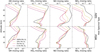 |
Fig. 5 Mixing ratio profiles of HOx (OH + HO2) and NOx (NO + NO2) species that power the catalytic cycles which destroy O3 for models with 100%, 10%, 1%, and 0.1% PAL O2. Here, we show models for the hottest (GOV) and coolest (M5V) stellar hosts. For decreasing O2 levels photolysis reaches lower levels of the atmosphere, causing OH and HO2 formation to occur at lower levels. The HOx is not significantly impacted by these changes since O3 formation is pushed deeper into the atmosphere as well. NOx species experience depletion via N2O and NO photolysis, although are less affected for models around cooler stars with lower photolysis rates. The efficiency of the NOx catalytic cycle decreases consistently for all host stars with decreasing O2 levels. See Sect. 4.3 for full details. |
4.3 Impact of varying O2 on catalytic cycles
Varying O2 levels impacts HOx (OH + HO2) and NOx (NO + NO2) species, which are the main contributors of catalytic cycles that destroy O3 (see Sect. 2.2 for details). Mixing ratio profiles of these species are shown in Fig. 5 for our hottest and coolest host stars. Once again, the impact on these species as O2 levels are decreased is controlled by photolysis reaching deeper levels of the atmosphere along with O(1D) production moving to lower levels as well.
As O2 decreases, HOx species (OH and HO2) in all models decrease in the upper atmosphere, but increase in the lower atmosphere. OH production via reactions with H2O (Reactions (8), (22)) and CH4 (Reaction (24)) occur at lower altitudes for lower O2 levels, especially since both H2O and CH4 are depleted in the upper atmosphere from photolysis. This “pushing down” of HOx species is more noticeable for hotter host stars with higher photolysis rates. Also note that stars with lower FUV/NUV ratios can better remove O3 via the HOx catalytic cycle, as FUV wavelengths create O3, while NUV wavelengths photolyze H2O to form OH. However, for all host stars the efficiency of the HOx catalytic cycle of O3 destruction is not largely impacted for different O2 and O3 abundances since OH and HO2 move down in the atmosphere along with O3 concentrations. Decreased O2 UV shielding and increased photolysis does not destroy HOx species, but rather converts them into other HOx species. When HO2 is photolyzed,
 (25)
(25)
it creates OH. The OH radical itself is extremely reactive with a short lifetime, and typically will react quickly with other species or react with O3 to create HO2 (Reaction (9)).
Although with decreasing O2 abundance HOx species are formed lower in the atmosphere rather than destroyed by photolysis, NOx species (NO + NO2) can be depleted via photolysis. The main source of NOx in the stratosphere is via N2Õ reactions with O(1D). However, as shown in Fig. 4, N2O is significantly depleted in the atmosphere via photolysis, especially for hotter host stars. While H2O, the primary source of HOx species in the stratosphere creates HOx during photolysis, N2O, the primary source of NOx species, does not. Instead it creates N2 and O(1D) (Reaction (20)), cutting off the main source of NO production from N2O. As for NOx species themselves, NO2 photolysis creates more NO, while NO photolysis simply breaks the molecule apart,
 (26)
(26)
 (27)
(27)
causing NO photolysis to be a sink of NOx. NO can be formed once again via reactions between N atoms and O2 molecules,
 (28)
(28)
although the rate of NO photolysis is faster than Reaction (28), causing it to be a gradual sink of NOx. Often the N atom created by Reaction (27) will remove NOx via,
 (29)
(29)
or the N atoms will recombine with other N atoms,
 (30)
(30)
with this reaction becoming more efficient as O2 levels drop. This sink via NO photolysis has less of an impact on cooler host stars with lower photolysis rates, hence less NOx depletion.
As seen in Fig. 5, NOx species are depleted throughout the atmosphere for the G0V host star, while the M5V host star experiences less NOx depletion, and actually an increase in NO in the lower stratosphere. This is due to primarily to lower photolysis rates for the cooler M5V star which depletes less N2O and NO (Reaction (14)). However, for model atmospheres around all host stars the ability of the NOx catalytic cycle to deplete O3 diminishes consistently with decreasing O2 levels, even for cooler stellar host models with less NOx depletion.
In summary, the HOx catalytic cycles are not hugely impacted by decreasing O2 because increased photolysis rates tend to push HOx species to lower altitudes rather than destroy them. However, NOx catalytic cycles decrease in efficiency with lower O2 levels since photolysis of N2O and NO remove NOx from the atmosphere.
UV integrated fluxes.
4.4 Surface UV flux for different O2 and O3 levels
Atmos was used to calculate the amount of UV flux reaching the planetary surface in each model atmosphere. Surface UV flux is strongly dependent on incident stellar Uv flux and the amount of UV shielding from both O2 and O3. High UV fluxes can cause substantial damage to biological organisms, hence UV surface environments will be critical for determining surface habitability. These results are summarized in Table 4 and shown in Fig. 6. Surface UV fluxes calculated here using a zenith angle of 60° (see Sect. 3.1).
Integrated surface UV fluxes are broken up into three biologically relevant wavelength regimes: UVA, UVB, and UVC. UVA flux (315–400 nm) is the lowest energy type of UV and is only partially shielded by O3, so a large percentage of incident UVA on modern Earth reaches the planetary surface. UVB (280-315 nm) is more harmful for life, contributing to sun burn and skin cancer in humans and damage to other organisms (e.g., Kiesecker et al. 2001). UVB is shielded much more efficiently by O3 than UVA, with a smaller fraction of incident UVB reaching the surface of modern Earth. UVC (121.6–280 nm) is capable of causing DNA damage, but is fortunately shielded almost entirely by O3 on modern Earth. Ozone is most efficient at shielding UV in this wavelength region, as evidenced by the O3 absorption cross sections shown in Fig. 1. We note that O2 photolysis, the first step in O3 formation (Reactions (1), (3)), requires a UVC photon (λ < 240 nm), allowing O2 to contribute partially to UVC shielding. However, since O3 is the primary shielder of UVC, the requirement of a UVC photon to produce O3 creates interesting correlations between incident and surface UVC flux.
Because UVA is not strongly shielded by O3, UVA surface fluxes for all models are closely correlated with the amount of incident UVA flux (see Table 4 and Fig. 6). For all host stars at O2 levels of 100%, 10%, 1%, and 0.1% PAL the amount of incident UVA that reaches the surface of these model planets is roughly ~80% for all cases. Because O3 plays only a small role in UVA shielding, all model results are quite similar.
UVB surface fluxes are significantly more variable because O3 shielding is much more important for these wavelengths. Although the G0V host star provides a higher incident UVB flux than the Sun, G0V-hosted models still maintain slightly less surface UVB flux until O2 decreases to 0.1% PAL, at which point the G0V and Sun model surface fluxes become roughly equal. This is due to the larger amount of O3 created by the G0V host star compared to the Sun, which allows for stronger UVB shielding (see Fig. 3 for O2–O3 relationship). The percentage of incident UVB flux that reaches the planetary surface varies significantly between different host stars. For our hottest host star (GOV) the amount of incident UVB flux reaching the planetary surface increases from 6.7% to 26.3% as O2 levels drop from 100% to 0.1% PAL. As a result of less O3 shielding, these percentages are higher for our coolest host star (M5V), which experiences an increase of 18.4% to 56.3% of incident UVB reaching the surface as O2 decreases from 100% to 0.1% PAL. Even though the cooler stellar hosts allow a higher percentage of UVB flux to travel through the atmosphere, they still maintain lower surface UVB values than hotter hosts due to their weaker incident UVB flux.
The strong reliance of UVC absorption on O3 abundance, along with the fact that O3 creation requires UVC photons, leads to some unexpected UVC surface flux results. A striking consequence of this is that while the GOV host star provides the highest incident UVC flux of all our host stars, it maintains the lowest surface UVC flux for the 100% PAL O2 model by several orders of magnitude, while the much cooler K2V stellar host model experiences the highest surface UVC flux. The much higher incident UVC flux of the GOV host causes much faster O3 production than other host stars, allowing for UVC shielding strong enough to counteract the high incident UVC flux. Another interesting result for the 100% PAL O2 case is that the M5V model has a slightly higher UVC surface flux than the K5V model, despite the fact that the M5V model has the lowest incident UVC flux. Again, this effect is due to the higher O3 abundance of the K5V-hosted planet, created by the stronger incident UVC flux. For all host stars, the atmospheric models with 100% PAL O2 allowed only extremely tiny fractions of incident UVC flux reach the surface (<10−17% in all cases).
UVC surface fluxes for models with 10% and 1% PAL O2 have similar trends when comparing stellar hosts. Sun-hosted models had the largest surface UVC fluxes in both scenarios. Notice that although the model atmospheres hosted by the G0V star and the Sun have higher O3 levels for the 10% PAL O2 cases compared to their 100% PAL O2 cases, overall UVC shielding is significantly less for the 10% PAL O2 cases due to the lesser contribution of O2 absorbing photons with wavelengths less than 240 nm. Even though the G0V host and the Sun produce much larger amounts of O3 than cooler stars, for low O2 levels the combined decrease in O2 and O3 UV shielding causes them to have higher surface UVC fluxes than cooler stars that produce significantly less O3. For model atmospheres with O2 levels of only 0.1% PAL, surface UVC levels begin to converge to the incident UVC flux as O2 and O3 levels have dropped enough that they shield UVC far less effectively. It has previously been suggested that the usefulness in the ability of O3 to shield UV drops off drastically at these O2 values (e.g., Segura et al. 2003). However, due to CO2 shielding, all models in this study had virtually no photons with wavelengths less than 200 nm reach the planetary surface, even with the lowest O2 abundance modeled (0.01% PAL).
Although the model atmospheres hosted by the hottest stars create the highest levels of O3, they constantly experience the highest UVA and UVB surface fluxes due to the limited shielding abilities of O3 in these wavelength ranges. However, for the far more damaging UVC wavelengths at 100% PAL O2 it is the G0V host star that provides the lowest UVC surface flux by orders of magnitude, with the Sun-hosted models having comparable UVC surface flux to cooler host star models. Somewhat ironically, for lower O2 levels of 1-10% PAL, it is the Sun that is the host star with the least “hospitable” conditions for surface life with the highest UVC surface fluxes. As O2 drops to 0.1% PAL UVC surface flux will begin to converge to the incident UVC flux as O2 and O3 shielding drops dramatically. However, though life on modern Earth requires a substantial O3 layer for UV protection, it is important to remember that evidence for life on Earth dates back to 3.7 Gyr ago (Rosing 1999), long before the O2 levels rose during the Great Oxidation Event 2.5 Gyr ago. The lack of significant atmospheric UV shielding may prevent life as we know it, but it does not rule out its existence. Life could exist, for instance, underwater, at a depth in which significant damaging UV has been absorbed by water (e.g., Cockell & Raven 2007).
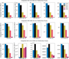 |
Fig. 6 Top-of-the atmosphere (TOA) and surface fluxes for UVA (top), UVB (middle), and UVC (bottom) wavelengths for 100%, 10%, 1%, and 0.1% PAL O2 model atmospheres for all stellar hosts. We note the differences in y-axis scale for different subplots. UVA flux is only slightly shielded by O3 so surface fluxes scale roughly with TOA fluxes. UVB flux is partially shielded by O3 and therefore allows the GOV-hosted models to receive less surface UVB than Sun-hosted models despite higher TOA UVB due to more efficient O3 production. UVC surface fluxes for high O2 levels are strongly influenced by O3 abundance due to strong UV shielding from O3 in this wavelength range. For models with only 0.1% PAL O2 levels all surface UV fluxes begin to converge to TOA values as the shielding of O3 is significantly decreased. See Sect. 4.4 for full details. |
4.5 O3 spectral features for different O2 levels
Emission spectra from our model atmospheres are shown in Fig. 7, zoomed in on the primary MIR O3 feature at 9.7 μm, along with the corresponding O3 mixing ratio and temperature profiles, which are necessary for interpreting the features. The temperature difference between the absorbing and emitting layers of the planet’s atmosphere, rather than the overall abundance of that gaseous species, determines the depth of planetary emission spectrum features. Because O3 is a main contributor of stratospheric heating, the strength of O3 features has a highly nonlinear relationship to O3 abundance. Once again, we see counterintuitive trends for hotter host stars (G0V, Sun, K2V), and different, more straightforward trends, for cooler host stars (K5V, M5V).
For all host stars, the 0.1% PAL O2 case has the shallowest O3 feature in emission spectra, but the O2 level for the deepest feature depends on the host star. For the G0V-hosted models the O3 feature for the 100% PAL O2 case has a similar depth to the 0.1% PAL O2 case, despite the fact that they have significantly different integrated O3 column densities (7.06 × 1018 cm−2 for 100% PAL O2; 1.23 × 1018 cm−2 for 0.1% PAL O2). For the two hottest host stars (G0V, Sun), the 10% and 1% PAL O2 cases are the deepest features. The strong features of the 10% PAL O2 models are not surprising since both the G0V and Sun models have higher O3 abundances at 10% PAL than at 100% PAL O2, but the 1% PAL O2 models have significantly less O3 than both the 10% and 100% PAL O2 cases (see Fig. 3 for reference). Conversely, O3 features for the coolest host star models correspond more intuitively to O2 and O3 levels, with the highest O2 and O3 abundances having the deepest features, and the lowest O2 and O3 abundances having the shallowest features.
The relationship between the depth of O3 spectral features and actual O3 abundance is dictated by atmospheric temperature profiles. The temperature difference between the emitting and absorbing layers of a gaseous species determines feature depth, therefore O3 feature depth is determined by the temperature difference between the altitude of peak O3 concentration in the stratosphere and the planet’s surface temperature. Because O3 NUV absorption is a dominant source of stratospheric heating, a higher O3 concentration with significant incident NUV flux for O3 to absorb results in higher stratospheric temperatures and thus a shallower spectral feature. This explains why an atmosphere with a large amount of O3 and high incident NUV flux (and more stratospheric heating) has a weaker O3 feature than an atmosphere with less O3 and weaker incident NUV, but a larger temperature difference between the stratospheric and surface temperatures. Cooler host star models with less O3 formation and lower incident NUV flux have significantly less stratospheric heating (Fig. 7), and therefore O3 spectral feature depths which correspond more strongly with the actual abundance of O3 in their atmospheres.
In summary, in order to interpret O3 features in planetary emission spectra and retrieve the O3 (and O2) abundances it will require modeling of the atmospheric temperature profiles. Both photochemistry and climate modeling will be essential in this process.
5 Discussion
5.1 Comparison to other studies
Multiple studies have explored O3 formation in Earth-like atmospheres using a variety of models, each providing valuable insight on the O2–O3 relationship. Here, we briefly describe relevant past studies on this topic. With 1D modeling of Earth’s atmosphere, early O3 studies revealed the nonlinear link between O3 and O2. Both Ratner & Walker (1972) and Levine et al. (1979) discuss the phenomenon of the O3 layer moving down in the atmosphere as O2 levels decreased (see Sect. 4.1 for details on this process) and agreed on peak O3 abundance occurring at ~10% PAL O2. Total O3 abundances calculated for these studies differed because they each included different chemical reactions. The model in Ratner & Walker (1972) contained only the Chapman mechanism, while Levine et al. (1979) additionally HOx and NOx catalytic cycle destruction of O3 in their model. Later Kasting et al. (1985) replicated the O3 peak in abundance at lower O2 levels using a more sophisticated model including chemistry beyond the Chapman mechanism and catalytic cycles, incorporating 20 gaseous species overall. They predicted maximum O3 production to occur at 50% PAL O2, a higher O2 estimate than previously. It is important to note that none of these studies included a climate model to calculate self-consistent atmospheric temperatures. Because the Chapman mechanism is temperature dependent, this helps account for discrepancies with later O3 calculations.
Studies in later years began to model O3 production in planetary atmospheres with different types of host stars. Segura et al. (2003) used what they described as a “loosely coupled” ID climate and photochemistry code (partially based off the Kasting et al. 1985 model) for different O2 levels around F2V, G2V, and K2V type stars. We note that this model is a predecessor of the model used in this study: Atmos. No host star displayed a peak O3 abundance at an O2 level less than 100% PAL, but this is likely because the modeled O2 levels were evenly spaced on a logarithmic scale from 0.001-100% PAL O2, whereas more finely spaced O2 levels are required to capture this effect. Atmospheric chemistry and temperature profiles computed in Segura et al. (2003) are similar to our Sun and K2V host star models. There are slight differences in total O3 abundance in these models compared to those in this study (our models tend to have lower O3), although this is likely due to differences in input UV spectra, boundary conditions, and model updates. Overall this is the most similar study to ours in terms of variety of O2 levels and host stars.
Other studies have also modeled O3 formation in Earth-like planetary atmospheres around different stellar hosts. The effect of varying orbital separations inside the habitable zone on O3 formation was explored for F2V, G2V, and K2V hosts (same as Segura et al. 2003) in Grenfell et al. (2007), and for a variety of M dwarfs in Grenfell et al. (2014). Both these studies used the ID “loosely coupled” climate and photochemistry model developed in Segura et al. (2003). An increase in star-planet separation for FGK stars caused cooler atmospheric temperatures, which correlated to an increase in O3. This is because the 3-body reaction that creates O3 (Reaction (2)) is faster at cooler temperatures. However, this O3 increase was not large because larger orbital distances also caused higher levels of HOx and NOx species which destroy O3 (Grenfell et al. 2007). When repeating this study for M dwarfs they found what they described as a “Goldilocks” effect in which there was a range of UV that was best for creating the most detectable O3. If incident UV flux is too low it will create small amounts of O3 making it harder to detect, but if the UV flux is too high it will create enough O3 to cause significant stratospheric heating, making it more difficult to detect in planetary emission spectra (see Sect. 4.5 details on this phenomenon). M7V spectral types were found to produce the amount of UV that was “just right” in creating detectable amounts of O3 (Grenfell et al. 2014). Although these models were run only at 100% PAL O2, their results are consistent with this study.
The impact of stellar host UV on O3 formation has also been modeled using Exo-Prime, a 1D coupled climate and photochemistry originally based off the same codes as Atmos, for Earth-like planets orbiting FGKM stars (Rugheimer et al. 2013), M dwarfs (Rugheimer et al. 2015a), cool white dwarfs (Kozakis et al. 2018), and red giants (Kozakis & Kaltenegger 2019). However, all these studies were constrained to O2 abundances of 100% PAL, although our corresponding models results are consistent. Another Exo-Prime study (Rugheimer et al. 2015b) modeled Earth at different points throughout geological history for FGKM stars, including four different O2 abundances, although the large variations in abundances of many gaseous species (i.e., CH4, CO2) does not allow for a straightforward comparisons of results with our study.
Of the 1D models discussed in this study, only Atmos models photochemistry in the mesosphere and lower thermosphere (up to an altitude of 100 km), whereas other photochemistry models are limited to atmospheric heights below ~65 km (Kasting & Donahue 1980; Kasting et al. 1985; Segura et al. 2003; Grenfell et al. 2007, 2014; Rugheimer et al. 2013, 2015a,b; Kozakis et al. 2018; Kozakis & Kaltenegger 2019). This is relevant for O3 formation because of the “secondary O3 layer” on Earth above the stratosphere (see details in Sects. 2 and 4.1). High energy photons (λ < 175 nm) are normally absorbed above the stratosphere by O2 photolysis, creating the O(1D) radical in the process (Reaction (3)). This could yield different findings for a photochemistry model that does not include higher altitudes since the high-energy photons will then be absorbed at far lower altitudes than in reality. This would change both the O(1 D) and O3 atmospheric profiles, and account for the differences in O3 production the we see from different models. However, overall results from the Segura et al. (2003) model, Exo-Prime, and Atmos remain fairly consistent.
Along with 1D models, O3 formation has been modeled in 3D. In reality, O3 formation and abundance is dependent on both the atmospheric latitude and time of day. On the night side of a planet, O3 cannot be generated by the Chapman method nor destroyed by photolysis. During the day O3 is created most efficiently at the equator where incident UV flux is highest, and then is transported toward the poles by Dobson-Brewer circulation, causing peak O3 abundance to vary in altitude depending on the latitude. On modern Earth, there is only a ~2% difference in O3 between the day and night sides, while planets with differing rotation periods may have more unevenly distributed O3. Despite the fact that 1D models (like ours) can use a zenith angle to represent the “average” of incoming radiation, they cannot accurately predict O3 formation and transport for slowly rotating planets, especially ones that are tidally-locked. Several studies have used 3D modeling to explore O3 formation and distribution on tidally locked planets. Proedrou & Hocke (2016) used a 3D climate and photochemistry model to compare O3 distribution on modern Earth and a tidally-locked version of Earth. They found that O3 could be distributed to the night-side of the planet and accumulate there in the absence of photolysis. Hemispheric maps of O3 distribution at different phases demonstrated that the amount of detectable O3 will be phase-dependent during observations.
Tidally-locked Earth-like planets are most likely found around lower mass stars, where the tidal-locking radius is within the habitable zone, and rotation periods are substantially shorter than the “tidally-locked Earth around the Sun” scenario investigated in Proedrou & Hocke (2016). Carone et al. (2018) used a 3D GCM to model how the rapid rotation of a tidally-locked planet would affect O3 transport on a planet with a 25-day period. This faster rotation created an “anti-Dobson-Brewer circulation” effect, with O3 accumulating at the equator rather than being transported toward the poles as on modern Earth. However, this study did not employ a photochemistry model, only circulation effects.
Chen et al. (2018) and Yates et al. (2020) also performed 3D modeling of tidally-locked habitable zone planets orbiting M dwarfs, although they incorporated both climate and photochemistry models as well. Chen et al. (2018) used CAM-Chem, a 3D model including 97 species in chemistry computations, while Yates et al. (2020) used the Met Office Unified Model including only Chapman mechanism and HOx catalytic cycle chemistry. Both studies found that O3 would be transferred to the night-side after being created on the day-side, where it could accumulate to a higher quantity than on the day-side. HOx species that were also transported to the night-side would be the primary sink of night-side O3. However, Yates et al. (2020) computed a thinner O3 layer than Chen et al. (2018), with the latter’s model also computing that O3 would exist at higher altitudes. These differences are likely due to differing chemical networks, land mass fraction (only Chen et al. 2018 had continents), and input stellar spectra. Overall these results agreed well with O3 abundances calculated by Rugheimer et al. (2015a) for a similar host star, although H2O mixing ratios (important for creating HOx species) were shown to vary significantly more, showing that 1D models do not include important feedback loops contained within 3D models.
The closest similar 3D modeling work to ours is Cooke et al. (2022), which uses a 3D climate-chemistry code to model the Earth-Sun system across geological history at various O2 levels from 0.1% to 150% PAL. Comparing their results to our Sun-hosted models there is agreement between trends in the time-averaged mixing ratios for different gaseous species. However, a main finding of Cooke et al. (2022) is that their 3D model predicts lower O3 abundances for O2 levels 0.5% to 50% PAL when compared to 1D models, including those calculated here as well as in Segura et al. (2003) and Rugheimer et al. (2015b). The cause for these lower estimates from this 3D model is uncertain, although is possibly related to how 1D codes simulate diurnal averages, or different CO2 abundances/boundary conditions. Further inter-model comparison will be needed in order to clarify these discrepancies (Cooke et al. 2022).
Overall our results for O3 formation are consistent with previous 1D studies and roughly similar to time-averaged results from 3D models. Despite this, it is important to remember that the night-sides of slowly rotating and tidally locked planets may have significantly more O3 than the day-side, introducing phase-angle dependency on the amount of detectable O3 for observations.
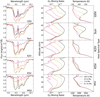 |
Fig. 7 Emission spectra, O3 mixing ratio profiles, and temperature profiles for model atmospheres with 100%, 10%, 1%, and 0.1% PAL O2 for all host stars. The depth of spectral features in emission spectra is dependent on the temperature difference between the absorbing and emitting layers of the atmosphere, causing the O3 feature depth to strongly correlate with the temperature difference between the stratosphere and planetary surface. However, since O3 is responsible for the majority of stratospheric heating, this results in higher O3 abundances (with more stratospheric heating) having shallower spectral features than atmospheres with less O3 and cooler stratospheres. For full details see Sect. 4.5. We note that temperatures for parts of the atmosphere above 1 mbar are held constant as that is the maximum height computed by the climate code (see Sect. 3.1 for more details). |
5.2 Factors that impact the O2–O3 relationship
The O2–O3 relationship is strongly dependent on the host star as well as the planetary atmospheric composition. Here we will briefly describe several ways the O2–O3 relationship can diverge from the results in this study.
We have shown that the O2–O3 relationship is highly influenced by the UV spectrum of the host star, both in terms of the total amount of UV flux and the FUV/NUV flux ratio, with FUV primarily responsible for creating O3, and NUV destroying it. In this study we selected stellar hosts from a range of spectral types, but have not yet explored the variation of UV activity and fUv/NUV ratios within specific spectral types. This is of particular importance for K and M dwarfs, as they are subject to larger amounts of UV variability, and thus greater variations in the O2–O3 relationship for the planets such stars host (e.g., France et al. 2013, 2016; Youngblood et al. 2016; Loyd et al. 2018). For instance, the UV spectrum for our M5V host star comes from GJ 876 which displays low amounts of chromospheric activity (France et al. 2016). If the stellar host in question was a more active star of a similar type, such as Proxima Centauri (classified as an M5.5V star; Boyajian et al. 2012; Anglada-Escudé et al. 2016), an orbiting Earth-like planet would be subject to a different O2–O3 relationship due to the significant change UV spectral slope of the star. A more in-depth study of the impact of varying UV activity levels for K and M dwarf planetary hosts will be necessary to fully understand how O3 production would vary for different O2 atmospheric abundances.
Another important aspect of this study to note is that the initial conditions of atmospheric species are kept constant across all models to better understand how the O2–O3 relationship differs for different host star spectra. However, the O2–O3 relationship could be altered by a variety of scenarios due to the potentially huge diversity of terrestrial planet atmospheric compositions.
The HOx and NOx catalytic cycles are the most prominent sinks for O3 on modern Earth, and could significantly impact O3 formation if there was an increase or decrease of the species powering these cycles. Therefore, changes in the amount of stratospheric H2O or N2O would alter the efficiency of O3 destruction, as they are the primary sources of stratospheric HOx and NOx. On modern Earth H2O is generally prevented from traveling into the stratosphere by the cold trap, although it can be created in the stratosphere via CH4 reactions with OH (Reaction (23)), implying a change in CH4 will additionally impact O3 destruction. The impacts on the O2–O3 relationship as these abundances change will be explored at length in the next paper of this series. Reducing gases in general (e.g., CH4, H2) can impact O2 and O3 levels, whether produced biologically or through volcanic outgassing (e.g., Hu et al. 2012; Black et al. 2014; Gregory et al. 2021; Cooke et al. 2022). O3 can also be depleted by cometary impacts (e.g., Marchi et al. 2021) and through solar flares (e.g., Pettit et al. 2018). In addition, O3 can vary throughout different seasons on modern Earth (Olson et al. 2018).
Oxygen-bearing species in general can also influence the O2–O3 relationship, especially in situations where O2 is produced abiotically via photolysis-driven production (see Meadows 2017 for full review). In particular, CO2-rich atmospheres may create significant amounts of O3 through CO2 photolysis (Hu et al. 2012; Domagal-Goldman et al. 2014; Tian et al. 2014; Harman et al. 2015; Gao et al. 2015) around host stars with high FUV/NUV flux ratios. FUV photons (λ < 200 nm) photolyze
 (31)
(31)
to produce an O atom (or the O(1D) radical if λ < 167 nm; Reaction (21)). Oxygen atoms can combine to create O2,
 (32)
(32)
which can then combine with O atoms to create O3 (Reaction (2)). Because O2 is photolyzed at shorter wavelengths than O3 (λ < 240 nm, see Fig. 1), stellar hosts with high incident FUV/NUV flux ratios can allow abiotic O3 accumulation without significant corresponding O2 buildup (Hu et al. 2012; Domagal-Goldman et al. 2014; Tian et al. 2014; Harman et al. 2015). In such scenarios the O3/O2 ratio would be higher than what would be predicted if O3 were formed directly from O2, implying that a high O3/O2 ratio could indicate non-biological O3 (and O2) creation (Domagal-Goldman et al. 2014). However, it remains uncertain which types of stellar hosts would be favorable for this scenario. Some studies find Sun-like stars can accumulate significant O3 through CO2 photolysis if outgassing rates of reduced species are low (Hu et al. 2012), while others restrict this scenario to K and M dwarfs with high FUV/NUV flux ratios (Tian et al. 2014; Harman et al. 2015). This scenario might likewise be produced by F star hosts with their strong FUV fluxes, although with enough NUV flux, O3 destruction rates could prevent O3 buildup (Domagal-Goldman et al. 2014). Differences in model lower boundary conditions, which control the impact of different O2 ground sinks, are likely to blame for the disparity in the capacity of O3 to accumulate between different studies (Domagal-Goldman et al. 2014; Tian et al. 2014; Harman et al. 2015; Meadows 2017). Despite uncertainties in O2 surface sinks, it is clear K/M dwarfs with high FUV/NUV ratios are susceptible, and potentially hotter stars with low abundances of reduced gaseous species. The effect of a CO2-rich atmosphere on the O2–O3 relationship will be highly influenced by the host star and atmospheric abundances of reduced gaseous species.
Another method of creating O3 without using the Chapman mechanism is via the “smog mechanism”, which can produce O3 photochemically using a volatile organic compound (i.e., CH4) and NOx. This process is responsible for smog pollution often occurring in large cities on modern Earth, but could also have occurred during the Proterozoic (2.5 Ga – 541 Ma) with high levels of CH4 and NOx (Grenfell et al. 2006). Under some circumstances Grenfell et al. (2006) computed that nearly double the amount of O3 on modern Earth could have been produced with just 1% PAL O2 via the smog mechanism. Additionally, Grenfell et al. (2013) found that the O3 smog mechanism may become more efficient than the Chapman mechanism for habitable zone planets around late M dwarf with low UV that is less efficient at O2 photolysis. Not only would O3 created primarily by the smog mechanism rather than the Chapman mechanism change the O2–O3 relationship, but “smog” O3 can be harmful for life. Smog mechanism O3 is created in the troposphere rather than the stratosphere, and could result in significant ground-level O3. Although on Earth our stratospheric O3 protects life by shielding harmful UV, ground level O3 on a smog-dominated planet can become fatal to Earth organisms at ~1 ppm.
Overall the O2–O3 relationship could be subject to large variations based both on the UV spectral slope of the host star, as well as atmospheric composition. Ozone formation via either CO2 photolysis or hydrocarbon reactions would not be expected to resemble the O2–O3 relationship that “Earth-like” atmospheres would demonstrate. However, the FUV/NUV flux ratio of the host star may allow us to rule out certain certain scenarios without observations of the planetary atmosphere.
5.3 Can we infer O2 abundance from an O3 measurement?
Returning to the question that prompted this study: is O3 a reliable proxy for O2? Variations in the O2–O3 relationship (Sect. 5.2) would increase the difficulty in using O3 to infer O2 abundance, and would require additional atmospheric information to provide the proper context. For the sake of simplicity, we will discuss the possibility of inferring O2 from an O3 measurement from our “Earth-like” models in this paper. But even in this simplified case where we keep initial conditions of all atmospheric species constant (apart from O2 and O3 and let them adapt to different stellar hosts) precisely determining O2 from O3 is not straightforward due to the nonlinear O2–O3 relationship.
Figure 3 clearly demonstrates that not only does the amount of O3 created for different O2 levels change significantly for different spectral types, but also the trend that the O2–O3 relationship will follow as O2 is changed will depend on the stellar host. Section 4.1 details how planets around hotter stars with higher UV flux (G0V, Sun, K2V) all experience their maximum O3 formation efficiency at O2 levels lower that 100% PAL, while there is a continuous (albeit nonlinear) decrease of O3 production for cooler hosts with lower UV flux (K5V, M5V). Whether a model atmosphere experiences an increase in O3 production as O2 decreases (as seen for hotter stars) is dependent primarily on whether O2 photolysis (λ < 240 nm) can reach deep into the atmosphere. The total amount of O3 depends on the FUV/NUV flux ratio of the host star as well, with FUV flux creating O3 while NUV wavelengths will cause its destruction (see Sects. 3.2 and 4.1). Although the K2V-hosted models demonstrate this effect with the maximum amount of O3 production occurring at 55% PAL O2, for models at O2 levels near 100% PAL O2 the K5V and M5V hosts have higher O3 abundances due to their larger FUV/NUV ratios. Therefore, to predict the O2–O3 relationship for a given star even with knowledge of “Earth-like” conditions knowing both the total UV emitted and UV spectral slope of the host star will be essential.
Idealized planetary emission spectra of the 9.7 μm O3 features in Fig. 7 show a non-trivial relationship between both O2 and O3 abundance and spectral feature depth for hotter stellar hosts, with more “straightforward” correlation of O2 and O3 abundances and feature depth for cooler hosts (K5V, M5V). This is due to the dependence of feature strength in emission spectra on the atmospheric temperature profile, with O3 measurements being particularly complicated by the fact that O3 highly influences stratospheric heating. Measuring O3 abundance from an emission spectra will require modeling of atmospheric temperature and pressure profiles for an accurate estimate, especially for stars emitting enough UV capable of creating and absorbing O3 for significant stratospheric heating. Smaller amounts of O3 as created by cooler stars have less of an impact on stratospheric heating, and therefore will maintain a more consistent temperature profile even for large variation in O2 abundance.
Even operating under the unlikely assumption that an accurate measurement of atmospheric O3 could be done, inferring O2 abundance will still not be straightforward, especially for hotter host stars (G0V, Sun, K2V) where O3 does not always decrease as O2 levels decrease. For example, in our Sun-hosted models the total integrated O3 column density at 150% PAL O2 is roughly the same as the amount at 5% PAL O2 (4.92 × 1018 cm−2 and 4.80 × 1018 cm-2, respectively). This implies that for hotter stellar hosts, it is unlikely O2 could be well constrained from an O3 measurement for relatively high levels of O2. It could, however, be possible to use an O3 measurement to differentiate between pre- and post-GOE O2 levels, as well as infer the existence of a substantial O3 layer providing surface UV shielding. Due to the consistent decrease in O3 abundance with decreasing O2 for cooler hosts, it appears that inferring O2 from O3 may be much simpler for planets orbiting cooler stars that those around hotter stars. It is important to note that specific knowledge of the UV spectral slope for cool K and M dwarfs will be extremely important to model O3 levels, especially due to the increased likelihood of O3 buildup via abiotic means and the diversity of activity levels (hence FUV/NUV flux ratios) around such stars.
5.4 is it necessary to constrain O2 abundance for O3 to be a useful biosignature?
Although inferring O2 levels precisely from O3 measurements will not be possible for hot stellar hosts and will still require additional atmospheric context and knowledge of the UV spectral slope for cooler hosts, what does this mean for O3 as a biosignature? Would it be necessary to infer O2 for O3 to be a useful indicator of life, or could it serve as a promising biosignature without precise O2 information? Two of the strongest arguments against O2 as a biosignature are 1) it can be produced abiotically, and 2) it has been at relatively high abundances for only a small fraction of Earth’s geological history (see review in Meadows 2017; Meadows et al. 2018b). We examine these arguments as they pertain to O3 as a biosignature.
The multiple proposed pathways for abiotic O2 production will prevent O3 from being a “standalone” biosignature as well. These mechanisms include production via CO2 photolysis as discussed in Sect. 5.3, as well as via H2O photolysis either from an extremely active pre-main sequence star (Luger & Barnes 2015; Tian 2015) or an atmosphere that has allowed H2O to enter the stratosphere due to a lack of cold trap from low abundances of non-condensable gases (Wordsworth & Pierrehumbert 2014). Ruling out these scenarios could be possible by detections or non-detections of gaseous species that would be produced or destroyed during these processes. For example, O2 and O3 abiotic buildup from CO2 photolysis could be revealed via a detection of CO, sometimes called an “antibiosignature” (for detailed descriptions of these mechanisms and their spectral discriminants see Meadows 2017; Meadows et al. 2018b).
Potential abiotic production will require contextual knowledge of an atmosphere to use either O2 or O3 as a biosignature. Abiotic buildup from CO2 photolysis with high FUV/NUV flux ratio stellar hosts could potentially impact O3 more than O2, as it is possible to accumulate O3 more easily than O2 in this scenario, and could potentially allow simultaneous detection of abiotic O3 and CH4 under certain conditions (Domagal-Goldman et al. 2014). However, predictions of abiotic O2 and O3 buildup are dependent on the lower boundary conditions of the model in question, so these estimates vary (Hu et al. 2012; Domagal-Goldman et al. 2014; Tian et al. 2014; Harman et al. 2015; Gao et al. 2015). Detections or non-detections of CO and CO2 will be important especially in assessing the origin of an O3 detection.
The second main argument against O2 as a reliable biosignature (even when accounting for abiotic sources) is that O2 levels have only been relatively high for a short period of Earth’s geological history. Oxygenic photosynthesis is thought to have been first used by cyanobacteria -2.7 Ga, although O2 buildup during the GOE was not thought to have occurred until ~2.5 Ga (e.g., Poulton et al. 2020). O2 levels comparable to modern Earth were not reached until the Phanerozoic (541 Ma – present day) sparked by the Cambrian explosion when land began to be colonized by plants (Lenton & Daines 2017; Dahl & Arens 2020). Before the GOE O2 levels were expected to be well below 10-3% PAL, and potentially remained relatively low during the majority of the Proterozoic (2.5 Ga–541 Ma) with estimates ranging from ~0.3–10% PAL O2 (e.g., Catling et al. 2018). Even if the lowest O2 estimates for the Proterozoic were reality (~0.01% PAL O2), there is evidence of an O3 layer after 2.4 Ga (Crockford et al. 2018). Although an O2 detection would be extremely difficult at this abundance, it has been suggested that O3 could reveal this undetectable O2 (e.g., Leger et al. 1993; Des Marais et al. 2002; Segura et al. 2003; Léger et al. 2011; Harman et al. 2015). Results of this paper only further prove this point, especially around hotter stars (see Fig. 3). For the G0V and Sun-hosted planets even at a level of 0.01% PAL O2, they still produce -15% the amount of O3 they do at 100% PAL O2. This number falls to -2% for the M5V-hosted planet, although it still demonstrates a less drastic decrease in O3 as O2 decreases. This implies that especially for planets orbiting hotter stars that O3 is a much longer lived detectable biosignature than O2 for an Earth-like planet, as detections may be sensitive to Proterozoic O3 levels.
Although gaining precise information about O2 abundance from an O3 measurement will be extremely difficult or not possible (see discussion in Sect. 5.3), knowing O3 abundance alone would still provide valuable information about the atmosphere. There appears to be a “bistability limit” for atmospheric O2, implying that certain O2 levels would not be stable in the atmosphere due to O2 sinks and geochemical cycles, as atmosphere switches from reduced to oxidizing (e.g., Segura et al. 2003; Goldblatt et al. 2006). Gregory et al. (2021) calculated that there are only a few stable solutions with O2 abundances between 3×10⁻⁶ and 1% PAL for an Earth-like planet orbiting the Sun. The existence of this “bistability limit” could explain the -300 Myr delay between the advent of oxygenic photosynthesis and appreciable O2 accumulation in the atmosphere (Goldblatt et al. 2006). O3 abundance drastically falls off for all our host stars under 0.01% PAL O2, implying that an O3 detection would allow us to distinguish between pre- and post-GOE O2 levels with relative ease. In the search for Earth-like planets, O3 appears to be a viable biosignature for a much longer portion of Earth’s history, potentially allowing us to infer the existence of oxygenic photosynthesis for much longer than an O2 detection.
Although O3 is not created by life, its UV shielding capabilities could allow estimates of whether the surface environment is safe for life. As seen in Fig. 6 and Table 4, the amount of UV flux reaching the planetary surface begins to converge quickly to the UV incident upon the planet when O2 abundance drops below 1% PAL, and it has been predicted that O2 levels less than this will not be efficient at preventing DNA damage (e.g., Segura et al. 2003). If an upper O2 “bistability limit” indeed exists at 1% PAL (Gregory et al. 2021), a detection of O3 in a planetary atmosphere could imply a certain amount of UV shielding, and potential surface life.
However, it is important to remember that the first evidence of life dates back 3.7 Ga, long before the GOE, or even oxygenic photosynthesis (Rosing 1999). Although O3 may be a longer lived biosignature than O2 and can indicate substantial UV surface shielding, a non-detection of O3 (or O2) could not rule out the existence of life. Although the surface UV environment would have been harsh before the GOE, it is possible that without a UV screen that life could thrive in the photic zone of the ocean, and perhaps colonize land (Cockell & Raven 2007). It has even been suggested that a significant amount of UV may have been necessary to synthesize prebiotic molecules (e.g., Patel et al. 2015; Ranjan & Sasselov 2016; Rimmer et al. 2018). Even substituting O3 for O2 in biosignature searches, life on pre-GOE Earth would be undetectable.
6 Conclusions
In this first part of our paper series we show that the nonlinear O2–O3 relationship varies significantly for model atmospheres of planets orbiting different types of host stars, with different trends for planets with hotter host stars versus those with cooler host stars. As seen in Fig. 3, planets orbiting hotter host stars display peak O3 abundance at lower O2 levels than modern Earth, while planets with cooler hosts have O3 decrease along with O2. The increase in O3 at lower O2 levels for hotter host stars is due to the O3 layer shifting downward in the atmosphere as O2 levels (and its ability to absorb UV) decrease. At these deeper and denser levels of the atmosphere the 3-body reaction that creates O3 (Reaction (2)) allows more efficient O3 production than at high O2 abundances. Cooler stars do not experience this effect since it requires a stronger incident FUV flux to push O3 formation deep enough in the atmosphere to allow for much faster production.
As O2 decreases in the atmosphere, photolysis of many gaseous species as well as O(1D) production will occur at lower atmospheric levels. The biologically relevant molecules H2O, CH4, and N2O all experience upper atmospheric depletion to different degrees, with these effects significantly more prominent around host stars with higher UV fluxes (Fig. 4). As O2 decreases and photolysis rates increase, HOx species are primarily pushed to lower altitudes rather than destroyed, while NOx species are destroyed by photolysis as well as produced at lower atmospheric levels (Fig. 5).
UVA and UVB wavelengths are only partially shielded by O3, so the amount of photons in this wavelength range that reach the planetary surface scales with the amount of incident UVA and UVB flux. However, for biologically damaging UVC photons, there is a much stronger dependence on both O2 and O3 abundance. For high O2 levels, our hottest host star (G0V) had the lowest surface UVC flux, despite also having the highest incident UVC flux (Fig. 6). As O2 and O3 abundances decreases these UVC surface levels begin to converge to incident UVC flux as UV shielding becomes inefficient.
Ozone features in planetary emission spectra were found to require knowledge of the atmospheric temperature profiles, as the depth of features is dictated by the temperature difference between the emitting and absorbing layers of the gaseous species. Since O3 NUV absorption is a significant source of stratospheric heating, a large amount of O3 along with significant incident NUV flux will cause a smaller temperature difference between the stratosphere and planetary surface, resulting in a shallower spectral feature (Fig. 7). For cooler stars with slower O3 production, and therefore less stratospheric temperature inversion, O2 spectral features are more intuitive to interpret. Overall it is clear that interpreting any observation of O3 will require the UV spectrum of the host star as well as photochemical and climate modeling of the planetary atmosphere.
Now that we have explored the O2–O3 relationship and its impact on planetary emission spectra, let us now return again to our original question: is O3 a reliable proxy for O2? In short, the complicated nature of the O2–O3 relationship tells us that O3 is not a reliable tracer of O2. Our results show us that for hotter stars, using O3 as a precise tracer for O2 will not be possible due to the degeneracies in the O2–O3 relationship, and for cooler stars it will be very difficult without knowledge of the UV spectrum of the host star as well as planetary atmospheric composition. However, an O3 measurement on its own is still an insightful measurement, even if it does not provide precise information on O2 abundance. Not only is O3 detectable in trace amounts (unlike O2), it additionally allows for an assessment of the UV surface environment of the planet.
There is likely no “standalone” atmospheric biosignature, but either O2 or O3 along with atmospheric context could provide evidence of oxygenic photosynthesis. Both will require detections of other gaseous species to rule out various mechanisms for abiotic O2 or O3 production. Although it is important to note that a CO2 rich planet may be more likely to have an abiotic buildup of O3 without O2 - a strike against O3 as a biosignature gas (see Sect. 5.2 for detailed discussion). However, there is a strike against O2 in comparison to O3:O2 has only existed on Earth in relatively high amounts for a short fraction of Earth’s geological history. Ozone, on the other hand, is detectable in trace amounts, potentially making it a longer lived detectable biosignature for Earth-like planets. It seems that neither O2 or O3 is inherently a “better” biosignature than the other; simply that they give different information and can be more or less useful depending on the scenario. With knowledge of the UV spectrum of the host star along with careful climate and photochemistry modeling we can begin to understand the O2–O3 relationship and use O3 as a reliable indicator for oxygenic photosynthesis.
Acknowledgements
We thank both the anonymous referee and journal editor for their comments which helped improve the clarity of this manuscript. All computing was performed on the HPC cluster at the Technical University of Denmark (DTU Computing Center 2021). This project is funded by VILLUM FONDEN.
References
- Anglada-Escudé, G., Amado, P. J., Barnes, J., et al. 2016, Nature, 536, 437 [Google Scholar]
- Arney, G., Domagal-Goldman, S. D., Meadows, V. S., et al. 2016, Astrobiology, 16, 873 [Google Scholar]
- Arney, G. N., Meadows, V. S., Domagal-Goldman, S. D., et al. 2017, ApJ, 836, 49 [NASA ADS] [CrossRef] [Google Scholar]
- Batalha, N. E., Marley, M. S., Lewis, N. K., & Fortney, J. J. 2019, ApJ, 878, 70 [NASA ADS] [CrossRef] [Google Scholar]
- Batalha, N., Rooney, C., & MacDonald, R. 2021, https://doi.org/10.5281/zenodo.5093710 [Google Scholar]
- Bétrémieux, Y., & Kaltenegger, L. 2013, ApJ, 772, L31 [CrossRef] [Google Scholar]
- Bétrémieux, Y., & Kaltenegger, L. 2014, ApJ, 791, 7 [CrossRef] [Google Scholar]
- Black, B. A., Lamarque, J.-F., Shields, C. A., Elkins-Tanton, L. T., & Kiehl, J. T. 2014, Geology, 42, 67 [NASA ADS] [CrossRef] [Google Scholar]
- Boyajian, T. S., von Braun, K., van Belle, G., et al. 2012, ApJ, 757, 112 [Google Scholar]
- Brasseur, G. P., & Solomon, S. 2005, Aeronomy of the Middle Atmosphere: Chemistry and Physics of the Stratosphere and Mesosphere (Dordrecht: Springer), 221 [Google Scholar]
- Carone, L., Keppens, R., Decin, L., & Henning, T. 2018, MNRAS, 473, 4672 [NASA ADS] [CrossRef] [Google Scholar]
- Catling, D. C., & Kasting, J. F. 2017, Atmospheric Evolution on Inhabited and Lifeless Worlds (Cambridge, UK: Cambridge University Press) [CrossRef] [Google Scholar]
- Catling, D. C., Krissansen-Totton, J., Kiang, N. Y., et al. 2018, Astrobiology, 18, 709 [NASA ADS] [CrossRef] [Google Scholar]
- Chapman, S. A. 1930, Mem. R. Met. Soc., 3, 103 [Google Scholar]
- Chen, H., Wolf, E. T., Kopparapu, R., Domagal-Goldman, S., & Horton, D. E. 2018, ApJ, 868, L6 [NASA ADS] [CrossRef] [Google Scholar]
- Cockell, C. S., & Raven, J. A. 2007, Phil. Trans. R. Soc. A., 365, 1889 [CrossRef] [Google Scholar]
- Cooke, G. J., Marsh, D. R., Walsh, C., Black, B., & Lamarque, J. F. 2022, Roy. Soc. Open Sci., 9, 211165 [NASA ADS] [CrossRef] [Google Scholar]
- Crockford, P. W., Hayles, J. A., Bao, H., et al. 2018, Nature, 559, 613 [NASA ADS] [CrossRef] [Google Scholar]
- Crutzen, P. J., & Lelieveld, J. 2001, Annu. Rev. Earth Planet. Sci., 29, 17 [CrossRef] [Google Scholar]
- Dahl, T. W., & Arens, S. K. 2020, Chem. Geol., 547, 119665 [NASA ADS] [CrossRef] [Google Scholar]
- Des Marais, D. J., Harwit, M. O., Jucks, K. W., et al. 2002, Astrobiology, 2, 153 [NASA ADS] [CrossRef] [Google Scholar]
- Domagal-Goldman, S. D., Segura, A., Claire, M. W., Robinson, T. D., & Meadows, V. S. 2014, ApJ, 792, 90 [CrossRef] [Google Scholar]
- DTU Computing Center 2021, DTU Computing Center resources [Google Scholar]
- Fauchez, T. J., Villanueva, G. L., Schwieterman, E. W., et al. 2020, Nat. Astron., 4, 372 [NASA ADS] [CrossRef] [Google Scholar]
- France, K., Froning, C. S., Linsky, J. L., et al. 2013, ApJ, 763, 149 [Google Scholar]
- France, K., Loyd, R. O. P., Youngblood, A., et al. 2016, ApJ, 820, 89 [NASA ADS] [CrossRef] [Google Scholar]
- Gao, P., Hu, R., Robinson, T. D., Li, C., & Yung, Y. L. 2015, ApJ, 806, 249 [NASA ADS] [CrossRef] [Google Scholar]
- Goldblatt, C., Lenton, T. M., & Watson, A. J. 2006, Nature, 443, 683 [CrossRef] [Google Scholar]
- Gregory, B. S., Claire, M. W., & Rugheimer, S. 2021, Earth Planet. Sci. Lett., 561, 116818 [CrossRef] [Google Scholar]
- Grenfell, J. L., Stracke, B., Patzer, B., Titz, R., & Rauer, H. 2006, Int. J. Astrobiol., 5, 295 [NASA ADS] [CrossRef] [Google Scholar]
- Grenfell, J. L., Stracke, B., von Paris, P., et al. 2007, Planet. Space Sci., 55, 661 [CrossRef] [Google Scholar]
- Grenfell, J. L., Gebauer, S., Godolt, M., et al. 2013, Astrobiology, 13, 415 [CrossRef] [Google Scholar]
- Grenfell, J. L., Gebauer, S., Paris, P., Godolt, M., & Rauer, H. 2014, Planet. Space Sci., 98, 66 [CrossRef] [Google Scholar]
- Harman, C. E., Schwieterman, E. W., Schottelkotte, J. C., & Kasting, J. F. 2015, ApJ, 812, 137 [NASA ADS] [CrossRef] [Google Scholar]
- Hu, R., Seager, S., & Bains, W. 2012, ApJ, 761, 166 [CrossRef] [Google Scholar]
- Kaltenegger, L., MacDonald, R. J., Kozakis, T., et al. 2020, ApJ, 901, L1 [NASA ADS] [CrossRef] [Google Scholar]
- Kasting, J. F. 1979, PhD thesis, University of Michigan, USA [Google Scholar]
- Kasting, J. F., & Ackerman, T. P. 1986, Science, 234, 1383 [NASA ADS] [CrossRef] [Google Scholar]
- Kasting, J. F., & Donahue, T. M. 1980, J. Geophys. Res., 85, 3255 [NASA ADS] [CrossRef] [Google Scholar]
- Kasting, J. F., Holland, H. D., & Pinto, J. P. 1985, J. Geophys. Res. 90, 10497 [NASA ADS] [CrossRef] [Google Scholar]
- Kiesecker, J. M., Blaustein, A. R., & Belden, L. K. 2001, Nature, 410, 681 [CrossRef] [Google Scholar]
- Kitzmann, D., Patzer, A. B. C., von Paris, P., Godolt, M., & Rauer, H. 2011, A&A, 531, A62 [NASA ADS] [CrossRef] [EDP Sciences] [Google Scholar]
- Kopparapu, R. K., Ramirez, R., Kasting, J. F., et al. 2013, ApJ, 770, 82 [NASA ADS] [CrossRef] [Google Scholar]
- Kozakis, T., & Kaltenegger, L. 2019, ApJ, 875, 99 [NASA ADS] [CrossRef] [Google Scholar]
- Kozakis, T., Kaltenegger, L., & Hoard, D. W. 2018, ApJ, 862, 69 [NASA ADS] [CrossRef] [Google Scholar]
- Kump, L. 2008, Nature, 451, 277 [NASA ADS] [CrossRef] [Google Scholar]
- Kurucz, R. L. 1979, ApJS, 40, 1 [NASA ADS] [CrossRef] [Google Scholar]
- Lederberg, J. 1965, Nature, 207, 9 [NASA ADS] [CrossRef] [Google Scholar]
- Leger, A., Pirre, M., & Marceau, F. J. 1993, A&A, 277, 309 [NASA ADS] [Google Scholar]
- Léger, A., Fontecave, M., Labeyrie, A., et al. 2011, Astrobiology, 11, 335 [CrossRef] [Google Scholar]
- Lenton, T. M. & Daines, S. J. 2017, Annu. Rev. Mar. Sci., 9, 31 [CrossRef] [Google Scholar]
- Levine, J. S., Hays, P. B., & Walker, J. C. G. 1979, Icarus, 39, 295 [NASA ADS] [CrossRef] [Google Scholar]
- Lin, Z., MacDonald, R. J., Kaltenegger, L., & Wilson, D. J. 2021, MNRAS, 505, 3562 [NASA ADS] [CrossRef] [Google Scholar]
- Lincowski, A. P., Meadows, V. S., Crisp, D., et al. 2018, ApJ, 867, 76 [NASA ADS] [CrossRef] [Google Scholar]
- Lippincott, E. R., Eck, R. V., Dayhoff, M. O., & Sagan, C. 1967, ApJ, 147, 753 [NASA ADS] [CrossRef] [Google Scholar]
- Lovelock, J. E. 1965, Nature, 207, 568 [NASA ADS] [CrossRef] [Google Scholar]
- Loyd, R. O. P., France, K., Youngblood, A., et al. 2018, ApJ, 867, 71 [Google Scholar]
- Luger, R., & Barnes, R. 2015, Astrobiology, 15, 119 [Google Scholar]
- Madden, J., & Kaltenegger, L. 2020, MNRAS, 495, 1 [CrossRef] [Google Scholar]
- Marchi, S., Drabon, N., Schulz, T., et al. 2021, Nat. Geosci., 14, 827 [NASA ADS] [CrossRef] [Google Scholar]
- Meadows, V. S. 2017, Astrobiology, 17, 1022 [CrossRef] [Google Scholar]
- Meadows, V. S., Arney, G. N., Schwieterman, E. W., et al. 2018a, Astrobiology, 18, 133 [Google Scholar]
- Meadows, V. S., Reinhard, C. T., Arney, G. N., et al. 2018b, Astrobiology, 18, 630 [Google Scholar]
- Misra, A., Meadows, V., & Crisp, D. 2014, ApJ, 792, 61 [Google Scholar]
- Olson, S. L., Schwieterman, E. W., Reinhard, C. T., et al. 2018, ApJ, 858, L14 [NASA ADS] [CrossRef] [Google Scholar]
- Patel, B., Percivalle, C., Ritson, D., Duffy, D., & Sutherland, J. 2015, Nat. Chem., 7, 301 [NASA ADS] [CrossRef] [Google Scholar]
- Pettit, J., Randall, C. E., Marsh, D. R., et al. 2018, J. Geophys. Res. (Space Phys.), 123, 5747 [NASA ADS] [CrossRef] [Google Scholar]
- Poulton, S. W., Bekker, A., Cumming, V., et al. 2020, Nature, 592, 232 [Google Scholar]
- Proedrou, E., & Hocke, K. 2016, Earth Planets Space, 68, 96 [CrossRef] [Google Scholar]
- Quanz, S. P., Absil, O., Benz, W., et al. 2021, Exp. Astron. [arXiv: 1908.01316] [Google Scholar]
- Ranjan, S., & Sasselov, D. D. 2016, Astrobiology, 16, 68 [CrossRef] [Google Scholar]
- Ranjan, S., Schwieterman, E. W., Harman, C., et al. 2020, ApJ, 896, 148 [Google Scholar]
- Ratner, M. I., & Walker, J. C. G. 1972, J. Atmos. Sci., 29, 803 [NASA ADS] [CrossRef] [Google Scholar]
- Rimmer, P. B., Xu, J., Thompson, S. J., et al. 2018, Sci. Adv., 4, eaar3302 [Google Scholar]
- Rosing, M. T. 1999, Science, 283, 674 [NASA ADS] [CrossRef] [Google Scholar]
- Rugheimer, S., Kaltenegger, L., Zsom, A., Segura, A., & Sasselov, D. 2013, Astrobiology, 13, 251 [NASA ADS] [CrossRef] [Google Scholar]
- Rugheimer, S., Kaltenegger, L., Segura, A., Linsky, J., & Mohanty, S. 2015a, ApJ, 809, 57 [Google Scholar]
- Rugheimer, S., Segura, A., Kaltenegger, L., & Sasselov, D. 2015b, ApJ, 806, 137 [NASA ADS] [CrossRef] [Google Scholar]
- Schwieterman, E. W., Kiang, N. Y., Parenteau, M. N., et al. 2018, Astrobiology, 18, 663 [CrossRef] [Google Scholar]
- Segura, A., Krelove, K., Kasting, J. F., et al. 2003, Astrobiology, 3, 689 [NASA ADS] [CrossRef] [Google Scholar]
- Segura, A., Kasting, J. F., Meadows, V., et al. 2005, Astrobiology, 5, 706 [Google Scholar]
- Segura, A., Walkowicz, L. M., Meadows, V., Kasting, J., & Hawley, S. 2010, Astrobiology, 10, 751 [Google Scholar]
- Selsis, F., Despois, D., & Parisot, J. P. 2002, A&A, 388, 985 [NASA ADS] [CrossRef] [EDP Sciences] [Google Scholar]
- Teal, D. J., Kempton, E. M. R., Bastelberger, S., Youngblood, A., & Arney, G. 2022, ApJ, 927, 90 [NASA ADS] [CrossRef] [Google Scholar]
- Tian, F. 2015, Earth Planet. Sci. Lett., 432, 126 [CrossRef] [Google Scholar]
- Tian, F., France, K., Linsky, J. L., Mauas, P. J. D., & Vieytes, M. C. 2014, Earth Planet. Sci. Lett., 385, 22 [CrossRef] [Google Scholar]
- Toon, O. B., McKay, C. P., Ackerman, T. P., & Santhanam, K. 1989, J. Geophys. Res., 94, 16287 [Google Scholar]
- Wordsworth, R., & Pierrehumbert, R. 2014, ApJ, 785, L20 [CrossRef] [Google Scholar]
- Wunderlich, F., Godolt, M., Grenfell, J. L., et al. 2019, A&A, 624, A49 [NASA ADS] [CrossRef] [EDP Sciences] [Google Scholar]
- Yates, J. S., Palmer, P. I., Manners, J., et al. 2020, MNRAS, 492, 1691 [NASA ADS] [CrossRef] [Google Scholar]
- Youngblood, A., France, K., Loyd, R. O. P., et al. 2016, ApJ, 824, 101 [Google Scholar]
- Zahnle, K., Claire, M. W., & Catling, D. 2006, Geobiology, 4, 271 [CrossRef] [Google Scholar]
All Tables
All Figures
|
Fig. 1 Absorption cross sections of O2 (left) and O3 (right), both plotted on the same y-axis scale to enable easier comparison. The y-axis is the same for both to enable easier comparison. Relevant O2 bands are the Schumann-Runge continuum (137–175 nm), the Schuman-Runge bands (175–200nm), and the Herzberg continuum (195–242nm). For less than 175nm an excited O atom, the O(1D) radical, is formed along with a ground state O atom during photolysis. O3 bands are the Hartley bands (200–300 nm), the Huggins bands (310–350 nm), and the Chappuis bands (410–750 nm). Photolysis within the Hartley bands will produce the O(1D) radical while other O3 bands create a ground state O atom. Absorption cross section data is from Brasseur & Solomon (2005). |
| In the text | |
|
Fig. 2 Stellar spectra of the planet host stars. G0V-K5V hosts are comprised of IUE UV data from Rugheimer et al. (2013), and the M5V host comes from UV observations of GJ 876 from the MUSCLES survey (France et al. 2016). Visible and IR wavelengths use ATLAS models of the same stellar temperature (Kurucz 1979). The right-hand figure zooms in on the UV region relevant for photolysis with important biological UV regimes (see Sect. 4.4). |
| In the text | |
|
Fig. 3 O2–O3 relationship for Earth-like planets orbiting different host stars (indicated in legend) with varying amounts of O2 mixing ratios. Molecular oxygen levels compared to Earth’s present atmospheric level (PAL) are shown as dashed vertical lines for reference. The left-hand figure shows the relationship in terms of total integrated O3 column density, and the right-hand figure in terms of total O3 normalized at the amount produced in the 100% PAL O2 case for each stellar host. The nonlinearity in these relationships is primarily due to the pressure dependence of Reaction (2) which forms O3. The main takeaway is that the O2–O3 relationship is significantly different for hotter host stars (GOV, Sun, K2V) versus cooler host stars (K5V, M5V), with hotter hosts experiencing peak O3 formation occurring at O2 levels under 100% PAL. See Sect. 4.1 for a detailed explanation. |
| In the text | |
|
Fig. 4 Mixing ratio profiles of O3, H2O, CH4, and N2O; all potential biosignature species. Each row represents results for model atmospheres orbiting different stellar hosts as indicated on the right-hand vertical axis. Each plot shows the mixing ratio profiles for O2 abundances of 100%, 10%, 1% and 0.1% PAL. O2 on modern Earth is a significant UV shield, allowing model atmospheres with decreasing O2 values to have photolysis occur at consistently lower altitudes. This is demonstrated well with the bulk of O3 forming at lower altitudes with less O2, as well as increased upper atmospheric depletion for H2O, CH4, and N2O via photolysis. The downward shift of O3 and upper atmospheric depletion of other species is shown to decrease for model atmospheres around cooler stars with lower incident UV flux, and hence lower photolysis rates. Full details of this atmospheric chemistry is shown in Sects. 4.1 and 4.3. |
| In the text | |
|
Fig. 5 Mixing ratio profiles of HOx (OH + HO2) and NOx (NO + NO2) species that power the catalytic cycles which destroy O3 for models with 100%, 10%, 1%, and 0.1% PAL O2. Here, we show models for the hottest (GOV) and coolest (M5V) stellar hosts. For decreasing O2 levels photolysis reaches lower levels of the atmosphere, causing OH and HO2 formation to occur at lower levels. The HOx is not significantly impacted by these changes since O3 formation is pushed deeper into the atmosphere as well. NOx species experience depletion via N2O and NO photolysis, although are less affected for models around cooler stars with lower photolysis rates. The efficiency of the NOx catalytic cycle decreases consistently for all host stars with decreasing O2 levels. See Sect. 4.3 for full details. |
| In the text | |
|
Fig. 6 Top-of-the atmosphere (TOA) and surface fluxes for UVA (top), UVB (middle), and UVC (bottom) wavelengths for 100%, 10%, 1%, and 0.1% PAL O2 model atmospheres for all stellar hosts. We note the differences in y-axis scale for different subplots. UVA flux is only slightly shielded by O3 so surface fluxes scale roughly with TOA fluxes. UVB flux is partially shielded by O3 and therefore allows the GOV-hosted models to receive less surface UVB than Sun-hosted models despite higher TOA UVB due to more efficient O3 production. UVC surface fluxes for high O2 levels are strongly influenced by O3 abundance due to strong UV shielding from O3 in this wavelength range. For models with only 0.1% PAL O2 levels all surface UV fluxes begin to converge to TOA values as the shielding of O3 is significantly decreased. See Sect. 4.4 for full details. |
| In the text | |
|
Fig. 7 Emission spectra, O3 mixing ratio profiles, and temperature profiles for model atmospheres with 100%, 10%, 1%, and 0.1% PAL O2 for all host stars. The depth of spectral features in emission spectra is dependent on the temperature difference between the absorbing and emitting layers of the atmosphere, causing the O3 feature depth to strongly correlate with the temperature difference between the stratosphere and planetary surface. However, since O3 is responsible for the majority of stratospheric heating, this results in higher O3 abundances (with more stratospheric heating) having shallower spectral features than atmospheres with less O3 and cooler stratospheres. For full details see Sect. 4.5. We note that temperatures for parts of the atmosphere above 1 mbar are held constant as that is the maximum height computed by the climate code (see Sect. 3.1 for more details). |
| In the text | |
Current usage metrics show cumulative count of Article Views (full-text article views including HTML views, PDF and ePub downloads, according to the available data) and Abstracts Views on Vision4Press platform.
Data correspond to usage on the plateform after 2015. The current usage metrics is available 48-96 hours after online publication and is updated daily on week days.
Initial download of the metrics may take a while.