| Issue |
A&A
Volume 699, July 2025
|
|
|---|---|---|
| Article Number | A270 | |
| Number of page(s) | 9 | |
| Section | Stellar atmospheres | |
| DOI | https://doi.org/10.1051/0004-6361/202555006 | |
| Published online | 14 July 2025 | |
Birthplaces of X-ray emission lines in Cygnus X-3
1
Dept of Physics,
PO Box 84,
00014
University of Helsinki,
Finland
2
Institutt for Fysikk, Norwegian University of Science and Technology,
Högskoleringen 5,
Trondheim
7491,
Norway
★ Corresponding authors: This email address is being protected from spambots. You need JavaScript enabled to view it.
; This email address is being protected from spambots. You need JavaScript enabled to view it.
Received:
2
April
2025
Accepted:
12
June
2025
Abstract
Aims. We investigate the formation of X-ray emission lines in the wind of the Wolf-Rayet (WR) companion in Cyg X-3 by analyzing their orbital dynamics using Chandra High Energy Transmission Grating (HEG) observations during a hypersoft state. Our goal is to constrain the X-ray transparency of the recently discovered funnel-like structure surrounding the compact star, as revealed by X-ray polarimetry.
Methods. We analysed Chandra/HEG observations and measured radial velocities and emission line intensities as a function of orbital phase for six emission lines: Si XIV 6.184 Å, S XVI 4.734 Å, Ar XVIII 3.731 Å, Ca XX 3.018 Å, Fe XXV 1.859 Å, and Fe XXVI 1.778 Å. We constructed radial velocity and emission intensity light curves for these lines using ten phase bins, which allowed us to investigate their orbital variability using a simple spherical WR-wind model.
Results. All lines exhibit sinusoidal orbital modulation, with the velocity amplitude generally increasing and the orbital phase with the highest blueshift generally decreasing for ions with a higher ionisation potential. The Fe XXVI-line displays velocity extremes at phase 0.25 (blueshift) and 0.75 (redshift), with a velocity amplitude of ~500 km/s, indicating that the line-emitting region is close to the compact component (disc or corona) and thus reflects the orbital motion. The Fe XXV-line shows a complex behaviour that cannot be fully resolved with the Chandra/HEG resolution. Other lines display velocity extremes scattered around phase 0.5 (blueshift) and 0.0 (redshift), with velocity amplitudes of 100–300 km/s, suggesting their origin in the WR stellar wind between the two components.
Conclusions. The Fe XXVI-line originates in the disc or corona of the compact object and can be used to constrain the system masses (Appendix A). The origin of the Fe XXV-line remains uncertain due to the limitations of Chandra/HEG resolution. The other lines formed in the WR-wind between the component stars, likely above the orbital plane along ionisation ξ-surfaces. Parts of the emission lines of Ar XVIII and Ca XX originated around the compact star. The wind-related component of the Ca XX line formed closest to the ionizing source (the compact star) due to its highest ionisation potential. The recent polarisation funnel-modelling is consistent with the present results during the hypersoft state.
Key words: atomic processes / binaries: general / stars: black holes
© The Authors 2025
 Open Access article, published by EDP Sciences, under the terms of the Creative Commons Attribution License (https://creativecommons.org/licenses/by/4.0), which permits unrestricted use, distribution, and reproduction in any medium, provided the original work is properly cited.
This article is published in open access under the Subscribe to Open model. This email address is being protected from spambots. You need JavaScript enabled to view it. to support open access publication.
1 Introduction
Cygnus X-3 (Cyg X-3; 4U 2030+40), one of the first X-ray binaries (XRBs) discovered (Giacconi et al. 1967), is among the brightest objects in both X-ray (e.g. Hjalmarsdotter et al. 2008; Szostek & Zdziarski 2008) and radio wavelengths (e.g. Waltman et al. 1994, 1996). It is a high-mass X-ray binary with a donor star (optical counterpart V1521 Cyg) that is likely a Wolf-Rayet (WR) star with a powerful radiatively driven wind, classified as either a WN 5–7 type star (van Kerkwijk et al. 1996) or a weak-lined WN 4–6 (Koljonen & Maccarone 2017). The relatively small size of this helium star allows for a tight orbit with a period of 4.8 hours (Parsignault et al. 1972). This characteristic is more typical of low-mass X-ray binaries, thus making Cyg X-3 a unique source in the Galaxy (Lommen et al. 2005). Recently, Veledina et al. (2024b) predicted the presence of a funnel around the X-ray source based on X-ray polarimetry. This funnel may influence the irradiation of the WR star and its surrounding wind as well as the observed X-ray continuum.
In this paper, we reanalyse Chandra High Energy Transmission Grating (HETG) observations taken during a hypersoft state (Koljonen et al. 2010, 2018) in January 2006 (initially analysed in Vilhu et al. 2009, hereafter Paper I). By studying the radial velocities and light curves of multiple emission lines, we aim to determine their formation sites and assess whether the funnel either leaks or channels X-ray flux from the compact object. We infer the formation sites by comparing the K-amplitudes and orbital phases with the highest blueshift of the emission lines with predictions from a spherical WR-wind model. Compared to Paper I, we employ a more refined continuum treatment, include additional emission lines, and address a new objective: identifying the birthplaces of X-ray emission features.
2 Chandra observations
Chandra HETG observations were conducted on January 25-–26, 2006, as part of a large international campaign to study Cyg X-3 during an active state (OBSID: 7268, PI: M. McCollough; see Paper I). The observations began on MJD 53760.59458 (corresponding to orbital phase 0.053) and continued until MJD 53761.42972 (orbital phase 4.240). During this period, Cyg X-3 was in a high-soft state (also known as the hypersoft state) with an average RXTE/ASM count rate of approximately 30 cps, equivalent to 400 mCrab. For comparison, typical hardstate count rates are below 10 cps.
We analysed data from the High Energy Grating (HEG), focusing on first-order spectra. The observation spanned more than four orbital cycles and was divided into ten phase bins. We concentrated on six emission lines: Si XIV 6.184 Å, S XVI 4.734 Å, Ar XVIII 3.731 Å, Ca XX 3.018 Å, Fe XXV 1.859 Å, and Fe XXVI 1.778 Å. These are not blends, and we could identify them using XSTAR1. Nearly all of these lines are hydrogen-like (H-like, with a single remaining electron) except Fe XXV, which is helium-like (He-like, with two remaining electrons). The spectral resolution was 0.012 Å, corresponding to velocity resolutions of 2020 km/s for the iron lines and 580 km/s for the Si XIV line. The lines are marked in Fig. 1, which shows the calibrated total flux at Earth (photons/s/keV/cm2). Mean emission line fluxes are given in Table 1, first row. The HEG first-order at 2 keV has an effective area around 100 cm2. Hence, on average one Si XIV-line photon was registered every 3.6 seconds.
These observations were also part of an extensive study on photoionisation emission models of Cyg X-3 (Kallman et al. 2019). The components of the Fe XXV line (resonance, intercombination, and forbidden) were recently analysed by Suryanarayanan et al. (2024) using a dataset similar to ours.
Results of the fitting procedures using a sine-curve for radial velocities and two absorbers for line intensities.
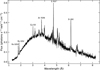 |
Fig. 1 Chandra/HEG spectrum (OBSID 7268). The lines we analysed are marked. The flux (F) is in units of photons/s/keV/cm2 at Earth. |
3 Orbital modulation of the emission lines
The emission lines can be approximated by single Gaussian profiles, except for the Si XIV line, which exhibits a clear P Cygni profile (Paper I). The sensitivity and resolution of Chandra (HEG) does not allow for the absorption components of other lines to be resolved. Thus, single Gaussian fits were used in this study. However, we also include the results obtained from modelling the Si XIV line with a P Cygni profile (Figs. 3–5). The spectra (photons/s/keV/cm2, see Fig. B.1) from ten orbital phase bins were transformed into velocity, V (km/s), coordinates relative to the rest-frame wavelength of each line (Vline km/s) and approximated using the following equation:
![Mathematical equation: $\[F(V)=F_{\text {cont }}(V)+A_0 \exp \left(\frac{-Z(V)^2}{2}\right),\]$](/articles/aa/full_html/2025/07/aa55006-25/aa55006-25-eq1.png) (1)
(1)
where Fcont(V) = A3 + A4(V − Vline) and Z(V) = (V − Vline − A1)/A2. The five parameters A0 (photons/s/keV/cm2), A1 (km/s), A2 (km/s), A3 (photons/s/keV/cm2), and A4 (photons/s/keV/cm2/(km/s)) were obtained by fitting the observed spectra using the IDL procedure MPCURVEFIT.PRO2. We note that the continuum at the line positions was included in the fits. The fitting was restricted to range between −10 000 km/s and 10 000 km/s. The line widths – full width at half maximum FWHM = 1.38A2 – are primarily instrumental (resolution-limited) and do not provide additional physical information. The fitted line profiles are shown in Fig. B.1.
The radial velocities, Vr (= A1 km/s), at ten orbital phases were fitted with a sine function:
![Mathematical equation: $\[V_r=B_0+B_1 ~\sin \left(2 \pi \phi+B_2\right).\]$](/articles/aa/full_html/2025/07/aa55006-25/aa55006-25-eq2.png) (2)
(2)
Here, ϕ is the orbital phase. This fit yielded the K-amplitude (= B1 km/s), the systemic velocity (= B0 = Γ km/s), and the phase at which the sine curve reaches its extrema (B2 = π and π/2 for maximum blueshift at phases 0.25 and 0.5, respectively).
The line emission Fem (photons/s/cm2) was obtained by integrating the second term in Eq. (1) between −6000 and 6000 km/s. We modelled this orbitally modulated total line emission as
![Mathematical equation: $\[F_{\mathrm{em}}=C ~\exp \left(-A_{\text {wind }} \tau_{\text {wind }}-A_{\text {clump }} \tau_{\text {clump }}\right),\]$](/articles/aa/full_html/2025/07/aa55006-25/aa55006-25-eq3.png) (3)
(3)
where we assumed that the line flux is absorbed by the same two components: the stellar wind and the so-called clumpy trail, which has been suggested to explain the orbital modulation of the X-ray and infrared continuum emission (Vilhu & Hannikainen 2013; Antokhin et al. 2022). We adopted the same phase-dependent profiles for dimensionless τwind and τclump as in Vilhu & Hannikainen (2013, their Fig. 5). The free parameters C (photons/s/cm2), dimensionless Awind, and Aclump were then determined using MPCURVEFIT.PRO. We also applied a similar fit to the X-ray continuum (co-adding Fcont between −6000 and 6000 km/s).
The fitting results are summarised in Table 1, with the last row providing chi-squared values for the radial velocity fits (DOF = 7). The value of Fem for the six lines, averaged over the orbital phase, are given in Table 1, first row. Some values of Table 1 can be compared with those reported in Paper I, which gives the K-amplitude and bluest phase for the Fe XXVI-line: 454 ± 108 km/s and 0.23±0.04, respectively. The corresponding values for the S XVI-line are 100±36 and 0.44±0.08. These values are consistent, within uncertainties, with those presented in Table 1. Minor differences can arise from different treatment of the continuum, which in the present paper is improved.
We note that the physical nature of the clumpy trail remains highly uncertain. It has been suggested to explain the observed decrease in the orbital modulation of the X-ray continuum at ϕ ~ 0.4 (Vilhu & Hannikainen 2013). In this scenario, the (conical) jet emission triggers the formation of dense clumps in the stellar wind, which are then advected along the wind to form a trail producing absorption at a narrow orbital phase interval. High-density clumps may prevent efficient cooling and enhance line absorption. The clumpy trail region is located at approximately 1.4 binary separations from the system’s centre and is crossed by the line of sight to the compact object at orbital phases between 0.2 and 0.6.
Figure 2 presents the radial velocity (left panels) and light curve fits (scaled by maximum value, right panels) for the six lines studied here. In the right-hand side panels, the continuum fits at the line positions are shown as dashed curves. We note that the rather unclear orbital modulation seen for the radial velocity of Fe XXV may stem from not resolving the absorption and emission components that are not in phase, as found recently by XRISM Collaboration (2024).
In Fig. 3 (upper panels), we plot the line ionisation potential (which correlates with their photon energy; see Table 1) with the K-amplitude and the orbital phase with the highest blueshift. Both show a relationship with the ionisation potential. As the ionisation potential increases, the K-amplitude increases from ~100 km/s to ~500 km/s, while the orbital phase with the highest blueshift decreases from ϕ = 0.6 to ϕ = 0.25. The Fe XXVI-line emitting region likely resides in the accretion disc or corona around the compact object, with the highest blueshift occurring at the orbital phase when the compact object is at its ascending node. Lower ionisation potential lines with modest K-amplitudes of 100–200 km/s and the orbital phases with the highest blueshift occurring at phases ϕ = 0.4–0.6 are more consistent in being located closer to the WR star and the centre of mass of the binary, where the stellar wind is still accelerating and the wind velocities are modest. The Ca XX line has a higher K-amplitude, indicating formation in a region with a higher wind velocity than the Ar, S, and Si lines.
In Fig. 3 (lower panels), we plot the line ionisation potential with the optical depths of the wind and clump absorbers. The clump absorption is significantly higher for the lines than for their corresponding continua (shown by filled boxes), while the opposite is true for wind absorption. The strong absorption by the clumpy trail (compared to continuum absorption) suggests that the gas in this region is highly ionised, enhancing line absorption. The Fe XXVI line exhibits the same wind absorption as its continuum, indicating a common formation site (compact star). The other emission lines likely originate above the orbital plane, as their wind absorption is lower than that of the continuum (see Fig. 3, lower-left plot).
Finally, we note that the continuum wind absorption depends on wavelength (or ionisation potential), as shown in Fig. 3 (lower-left plot). This behaviour resembles the differences observed between soft and hard X-ray light curves (Vilhu et al. 2003; Zdziarski et al. 2012). Pure wavelength-independent Thomson scattering alone cannot fully explain this trend.
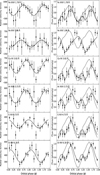 |
Fig. 2 Sine curve fits for the radial velocity (km/s, left panels) and two-absorber fits for the line emission (scaled, photons/s, right panels) for the six analysed emission lines. The dashed line represents the continuum at the line. |
4 Sites of line formation
In this section, we study the potential locations for the line emission in more detail. To obtain a rough estimate, we created a rotating grid of mesh points in the orbital (x,y) plane between the stars and computed radial velocities within this grid. In this coordinate system, the x-axis connects the stars, the y-axis is perpendicular to it, the WR star is located at (x,y) = (0,0), and the compact object is at (1,0). The coordinate system rotates counter-clockwise around the WR centre over the 4.8-hour orbital period. The grid consists of 80 × 80 points spanning from (x,y) = (0,−0.5) with a uniform step size of Δx = Δy = 0.014.
The wind velocity was modelled using the β-law:
![Mathematical equation: $\[v_{\text {wind }}=v_{\infty}\left(1-R_{\text {star }} / r\right)^\beta,\]$](/articles/aa/full_html/2025/07/aa55006-25/aa55006-25-eq4.png) (4)
(4)
where v∞ = 1600 km/s and β = 1.0, which are values consistent with WNE stars in the Potsdam models3. We adopted an orbital inclination of i = 30° (Vilhu et al. 2009; Antokhin et al. 2022; Veledina et al. 2024a, see also Appendix A).
At each grid point, we computed the K-amplitude and the orbital phase of the highest blueshift, then compared these values with the observed parameters of the six emission lines listed in Table 1. This analysis is illustrated in Fig. 4. In the top panel of Fig. 4, the K-amplitudes of the grid points are plotted as a function of their y-values. Curves are labelled by the corresponding x-coordinate. The middle panel shows the corresponding orbital phases of the highest blueshift. Observed values from Table 1 are indicated in both panels by dashed horizontal lines. In the figure, ‘Si2G’ refers to a two-Gaussian fit (emission plus absorption, i.e. P Cygni profile). The bottom panel summarises the inferred formation regions by combining information from the top two panels, including error estimates derived from the data. Dotted contours indicate constant K-amplitudes and orbital phases with highest blueshift. In practice, the likely formation site of each emission line corresponds to the intersection of contours representing its observed K-amplitude and bluest phase, as listed in Table 1.
The plot in the bottom panel of Fig. 4 depicts the system at phase ϕ = 0 as viewed from below. The plot is on the orbital plane (z = 0). However, the birth sites are briefly the same when using z = ±0.3. The birthplaces of the Ca XX and Ar XVIII lines are not symmetrically located between the stars because their orbital phase with the highest blueshift clearly occurs before phase 0.5. This may indicate that a part of them formed near the compact star, which we examine in the next section.
We assumed that the Ca and Ar lines originate from two locations: the stellar wind, where the maximum blueshift occurs at phase ϕ = 0.5, and another region near the compact star, where the maximum blueshift occurs at phase ϕ = 0.25. Additionally, we assumed that the Fe XXVI line formed entirely in the vicinity of the compact star (disc or corona). This is also supported by XSTAR wind-simulations, which do not provide enough Ar XVIII, Ca XX, and Fe XXVI line photons (see Fig. 2 in Paper I). The observed radial velocity curve can then be expressed as the sum of the contributions from line emission at both the wind and compact star locations:
![Mathematical equation: $\[\begin{aligned}& K ~\sin \left(2 \pi \phi+\phi_{\max, \text { blueshift }}\right) \\& \quad=f K_{\text {wind }} ~\sin (2 \pi \phi+\pi / 2)+K_{\mathrm{CS}} \times(1-f) ~\sin (2 \pi \phi+\pi).\end{aligned}\]$](/articles/aa/full_html/2025/07/aa55006-25/aa55006-25-eq5.png) (5)
(5)
Here, f is the fraction of the line emission attributed to the wind location, while the values for K and ϕmax,blueshift can be found in Table 1 for each line. We used KCS = KFeXXVI = 484 km/s (see Table 1) and solved for f and Kwind. In the case of Ca XX, we obtained Kwind = 470 km/s and f = 0.5, indicating that half of the line photons formed in the wind in a region with a relatively high velocity and the other half formed at the compact star. For Ar XVIII, we obtained Kwind = 140 km/s and f = 0.7, indicating that the majority of the line emission is consistent with arising from the wind close to the WR companion.
The alternative line formation sites in the stellar wind consistent with the derived parameters are illustrated in Fig. 5. The K-values of the S and Si lines were obtained by fixing their bluest phases to ϕ = 0.5. These values are not significantly different from those in Table 1.
Errors were propagated from uncertainties in K-amplitudes and ϕmax,blueshift. We also plot the constant ionisation parameter surfaces, ![Mathematical equation: $\[\xi=L_{X} /\left(N r_{C S}^{2}\right)\]$](/articles/aa/full_html/2025/07/aa55006-25/aa55006-25-eq6.png) in the figure while assuming a spherically symmetric X-ray emission from the compact star. Here, L is the ionizing luminosity, estimated as L = 2.46 × 1038 erg/s (Paper I); N is the gas number density; and rCS is the distance from the compact star. In mass-conserving, spherical, and isotropic wind, the mass-loss rate is given by
in the figure while assuming a spherically symmetric X-ray emission from the compact star. Here, L is the ionizing luminosity, estimated as L = 2.46 × 1038 erg/s (Paper I); N is the gas number density; and rCS is the distance from the compact star. In mass-conserving, spherical, and isotropic wind, the mass-loss rate is given by ![Mathematical equation: $\[\dot{M}=4 \pi r^{2} \rho v_{\text {wind}}\]$](/articles/aa/full_html/2025/07/aa55006-25/aa55006-25-eq7.png) , where the wind density depends on the distance from the WR centre as
, where the wind density depends on the distance from the WR centre as ![Mathematical equation: $\[\rho \propto r_{W R}^{-2} / v_{\text {wind}}\]$](/articles/aa/full_html/2025/07/aa55006-25/aa55006-25-eq8.png) . We computed vwind using Eq. (4).
. We computed vwind using Eq. (4).
Assuming a wind mass-loss rate of ![Mathematical equation: $\[\dot{M}=10^{-5} M_{\odot}/year\]$](/articles/aa/full_html/2025/07/aa55006-25/aa55006-25-eq9.png) (Koljonen & Maccarone 2017) and a mean molecular weight of μ = 1.33 for ionised helium gas, we could derive the constant ionisation surfaces in Fig. 5 in the range log ξ = 2.0–5.0, which covers the equilibrium values for our observed lines (Si XIV: log ξ = 2.0–3.5, Ca XX: log ξ = 2.5–4.5, as given in the XSTAR manual). Assuming a wind consisting mostly of singly ionised helium (μ = 1.75), the above ranges would change only modestly (increased by 0.12). In addition, we expect that the HeII-ions are formed at the far side of the WR wind with respect to the compact star (in the X-ray shadow); this is supported by infrared observations from Koljonen & Maccarone (2017, their Fig. 8). Using the methods described in this paper, the inferred formation sites of the HeII lines lie near (x,y) = (—0.55, 0) based on the K-amplitude of 400 km/s and orbital phase 0.0 at the highest blueshift.
(Koljonen & Maccarone 2017) and a mean molecular weight of μ = 1.33 for ionised helium gas, we could derive the constant ionisation surfaces in Fig. 5 in the range log ξ = 2.0–5.0, which covers the equilibrium values for our observed lines (Si XIV: log ξ = 2.0–3.5, Ca XX: log ξ = 2.5–4.5, as given in the XSTAR manual). Assuming a wind consisting mostly of singly ionised helium (μ = 1.75), the above ranges would change only modestly (increased by 0.12). In addition, we expect that the HeII-ions are formed at the far side of the WR wind with respect to the compact star (in the X-ray shadow); this is supported by infrared observations from Koljonen & Maccarone (2017, their Fig. 8). Using the methods described in this paper, the inferred formation sites of the HeII lines lie near (x,y) = (—0.55, 0) based on the K-amplitude of 400 km/s and orbital phase 0.0 at the highest blueshift.
The wind on the face-on side is significantly influenced by X-rays from the compact star. In particular, the EUV flux below the HeII ionisation edge at 54.4 eV (228 Å) plays a critical role in regulating the ionisation of species responsible for the radiative line driving (primarily NiV, FeV, CIV, NV, and CrV; Vilhu et al. 2021, their Appendix B). When the EUV flux is strong, these ions become fully ionised, reducing or eliminating the line-driving force.
During the hypersoft state of Cyg X-3, this ionisation occurs roughly halfway between the WR and the compact star, creating a kink in the wind velocity profile (Vilhu et al. 2023). We note that the wind velocities in Fig. 2 of that study were computed without including the gravitational pull of the compact star in order to facilitate accretion modelling, so they only reflect the impact of the reduced line force. Including the gravitational attraction of the compact star would (over)compensate the loss in line force. Nevertheless, this kind of wind suppression model does not alter the qualitative conclusions of the present model, though it may shift the inferred Ca XX line formation sites slightly closer to the WR star.
Using constant ionisation ξ-surfaces, we can investigate the K-amplitude values over the entire surface, weighting local velocities by the wind density. The derived K-amplitude values, with bluest phases at 0.5, do not alter the qualitative conclusions of this paper.
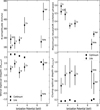 |
Fig. 3 K-amplitude (upper-left), the orbital phase with the highest blueshift (upper-right), Awind (lower left), and Aclump (lower right) as a function of the ionisation potential of the ion. Dots with error bars show the emission lines, while the filled boxes indicate the continua at the lines. ‘Si2G’ in the upper panels denotes the P Cygni (two-Gaussian) solution for the Si XIV line. |
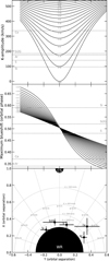 |
Fig. 4 Top panel: K-amplitudes of grid points plotted against their y-values sorted by their x-values. Middle panel: same as the upper panel but for the orbital phases with the highest blueshift. The values corresponding to the observed emission lines are marked by horizontal lines. Bottom panel: line formation sites combining information from the two upper panels (dots with error bars). The bottom panel also shows (dotted) curved contours with constant K-values (200, 300, 400, and 500 km/s increasing from the WR surface) and radial (dotted) contours with the constant bluest phases ϕ (from 0.3 to 0.7). |
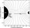 |
Fig. 5 Alternative arrangement for the emission regions of the Si XIV, S XVI, Ar XVIII, and Ca XX lines. Parts of the Ca and Ar lines formed in the compact star disc or corona (see the text). The solid curves represent surfaces with a constant ionisation parameter marked by a log ξ-value. These curves are intersections with the (x,y) plane of 3D surfaces where the lines are expected to form. For clarity, the error bars have been shifted vertically from y=0. The coordinate system is the same as in Fig. 4. |
5 Discussion
5.1 Sensitivity of the parameter values on the emitting locations
In this section, we discuss relaxing some of the assumptions used in the above modelling. Concerning the wind velocity law, we also repeated computations with smaller β values and found that the only difference was that the emission locations were closer to the WR star. Furthermore, the same effect was observed when using the X-ray suppressed wind model proposed by Vilhu et al. (2021) (if the gravitational pull of the compact star is included). Similarly, a larger orbital inclination (>30°) produced the same effect. We did not account for the impact of the WR star’s orbital motion around the centre of mass on wind velocity. However, this effect is expected to be small since the mass ratio is large (see Appendix A) and the centre of mass lies inside the WR companion.
Most likely, the sizes of the actual line emitting regions are much more extended than those shown in Figs. 4 and 5, which are based on the closest matches between observed K-values and orbital phases of the highest blueshift at individual grid points. These values likely represent an average of many regions. A co-added combination of multiple grid points, weighted by density and photoionisation effects, can also reproduce the observed K-values and orbital phases of the highest blueshift. However, without a detailed photoionisation study (such as that in Kallman et al. 2019), the precise sizes and locations of the emitting regions remain difficult to map.
5.2 Implications for the system geometry at the compact star
The emitting regions of the lines could provide constraints on the potential funnel structure around the compact star (Veledina et al. 2024b), as this funnel must produce or leak sufficient ionizing radiation to illuminate the WR wind on the side facing the compact star. Based on Veledina et al. scenario (see their Fig. 5), this appears to be the case, at least in the hypersoft state, where radiation is primarily scattered (single scattering) off the material along the funnel axis, rather than being dominated by emission reflected from the funnel walls. For X-rays in the keV range, the Klein-Nishina formula predicts scattering in all directions. The observed reduction of X-ray polarisation in the hypersoft state could also arise from the effects of matter ionisation, in which case the funnel becomes partially transparent to the reflected radiation.
We note that the low-hard state X-ray spectra reveal spectral lines similar to those shown in the hypersoft state (scaled with the continuum; Kallman et al. 2019). This may already indicate that the funnel walls in the hard state are also at least partially transparent.
5.3 Issues in determining the parameters for Fe XXV emission region
As noted above, the birthplace for the Fe XXV line remains problematic and cannot be reliably determined with the Chandra/HEG resolution. Notably, phase-dependent radiative transfer effects and variations in the line components (intermediate, resonance, and forbidden) may obscure any Doppler motion related to the line formation region.
Observations with the XRISM/Resolve spectrometer, which offers unprecedented spectral resolution, have shown that emission and absorption lines can be distinguished (XRISM Collaboration 2024). The emission lines in the 6–9 keV range originate from a region with a medium ionisation parameter (log ξ ≈ 3) and exhibit radial velocity modulation with K = 194 ± 29 km/s, and they reach the highest blueshift at the orbital phase ϕ = 0.25 (though the Fe XXV line should be separated from the Fe XXVI line). The absorption lines show a much weaker orbital modulation, with K = 55 ± 7 km/s, but they have a significantly higher systemic velocity (Γ = −534 ± 6 km/s). Their radial velocity extrema occur at orbital phases ϕ = 0.1 (maximum) and ϕ = 0.6 (minimum), suggesting they originate from a larger region with a size scale comparable to the binary orbit.
6 Conclusions
We have analysed Chandra/HEG observations of Cyg X-3 during a hypersoft state. We determined radial velocities and emission line intensities as a function of orbital phase for six X-ray emission lines: Si XIV 6.184 Å, S XVI 4.734 Å Ar XVIII 3.731 Å, Ca XX 3.018 Å, Fe XXV 1.859 Å, and Fe XXVI 1.778 Å (Fig.1).
Assuming a spherical wind and a two-component absorbing model, we determined the potential emission regions for the studied lines. As in Paper I, we assumed that the iron line Fe XXVI originates in the compact star disc or corona and that the radial velocity curve reflects its orbital motion. In Appendix A, this is used to constrain system parameters. The origin of the Hetype iron line, Fe XXV, remains unresolved due to the insufficient resolution of Chandra/HEG.
We find that the other lines likely formed within the WR wind between the two stellar components, with their radial velocities reflecting wind velocities. Parts of Ca XX and Ar XVIII emissions originate in the disc or corona of the compact star, with their radial velocities representing a mixture of wind and orbital motions. This is also supported by XSTAR wind-simulations (Paper I, Vilhu et al. 2009). The ionisation parameter, ξ, required to achieve a given ionisation state is higher for high-Z elements than for lower-Z elements (Kallman et al. 2019). Consequently, the wind component of the Ca XX line emission is located closer to the compact star than the other lines (Fig. 5).
The line-emitting regions are also likely located in the upper half of the (more or less spherical) ionisation ξ-surfaces, as their wind absorption is weaker than that of the continuum originating from the compact star. Assuming different wind models (e.g. lower β values) shifts the line formation sites closer to the WR star. A similar effect occurs if the system inclination is higher than 30° (for a discussion on inclination, see Appendix A).
The funnel model around the compact star by Veledina et al. (2024a) appears to allow wind ionisation at these sites, at least during the hypersoft state. Whether the funnel walls remain transparent during the quiescent hard state remains to be studied.
Acknowledgements
This project has received funding from the European Research Council (ERC) under the European Union’s Horizon 2020 research and innovation programme (grant agreement no. 101002352). We thank the referee for very useful comments.
Appendix A Component masses and inclination
Assuming that the Fe XXVI line originates close to the compact star (disc/corona), we can derive the WR mass function from the K-value of Kc = 484 ± 95 km/s (Table 1):
![Mathematical equation: $\[f_{\mathrm{WR}}=\frac{K_c^3 P}{2 \pi G}=2.35_{-1.14}^{+1.66} M_{\odot} \equiv \frac{M_{\mathrm{WR}}^3 ~\sin ^3 i}{M_{\mathrm{tot}}^2},\]$](/articles/aa/full_html/2025/07/aa55006-25/aa55006-25-eq10.png) (A.1)
(A.1)
where P = 17 253 s is the orbital period (Antokhin & Cherepashchuk 2019), G is the gravitational constant, i is the orbital inclination (the angle between the line of sight and the orbital plane axis), and MWR and Mtot are the WR and total system masses, respectively. This value is slightly larger than that computed in Paper I, where a compromise was made in phase binning (see also Zdziarski et al. 2013).
Hanson et al. (2000) observed infrared He I absorption lines with a K-amplitude of KWR = 109 ± 13 km/s. They favour the interpretation that these lines are centred on or associated with the motion of the WR-star (however, see discussion in Koljonen & Maccarone 2017 with possible caveats on the detection of this line). Using this K-value, the mass function of the compact star can be derived as
![Mathematical equation: $\[f_{\mathrm{c}}=\frac{K_{\mathrm{WR}}^3 P}{2 \pi G}=0.027_{-0.008}^{+0.011} M_{\odot} \equiv \frac{M_{\mathrm{c}}^3 ~\sin ^3 i}{M_{\mathrm{tot}}^2},\]$](/articles/aa/full_html/2025/07/aa55006-25/aa55006-25-eq11.png) (A.2)
(A.2)
where Mc is the compact star mass.
Dividing these two mass functions gives the mass ratio
![Mathematical equation: $\[\frac{M_c}{M_{\mathrm{WR}}}=\frac{K_{\mathrm{WR}}}{K_c}=0.23_{-0.04}^{+0.06}.\]$](/articles/aa/full_html/2025/07/aa55006-25/aa55006-25-eq12.png) (A.3)
(A.3)
Substituting Eq. (A.3) into Eq. (A.1) and assuming an inclination of 30 degrees, we obtain the WR mass: ![Mathematical equation: $\[M_{\mathrm{WR}}=28_{-12}^{+17} ~M_{\odot}\]$](/articles/aa/full_html/2025/07/aa55006-25/aa55006-25-eq13.png) . This corresponds to a compact object mass of
. This corresponds to a compact object mass of ![Mathematical equation: $\[M_{\mathrm{c}}=6.3_{-2.0}^{+2.5} ~M_{\odot}\]$](/articles/aa/full_html/2025/07/aa55006-25/aa55006-25-eq14.png) . As with all values determined above, we report the mean and the 16%–84% confidence interval of the resulting parameter distribution. The 0.2%–99.8% interval (3σ) is 3.6 M⊙ < MWR < 96 M⊙ and 1.7 M⊙ < Mc < 15 M⊙.
. As with all values determined above, we report the mean and the 16%–84% confidence interval of the resulting parameter distribution. The 0.2%–99.8% interval (3σ) is 3.6 M⊙ < MWR < 96 M⊙ and 1.7 M⊙ < Mc < 15 M⊙.
If Eq. (A.2) cannot be trusted, we can instead use Eq. (A.1) and an inclination of 30 degrees to determine a limiting minimum WR mass for which the compact star mass is at least that of a neutron star (Mc ≥ 1.4 M⊙): ![Mathematical equation: $\[M_{\mathrm{WR}} \geq 21_{-9}^{+14} ~M_{\odot}\]$](/articles/aa/full_html/2025/07/aa55006-25/aa55006-25-eq15.png) . At the 3σ level, MWR > 3.2 M⊙. We note that the total mass of the binary, which can be estimated from the orbital decay and the WR mass-loss rate, is constrained to Mtot ≲ 20 M⊙ (Zdziarski et al. 2013; Koljonen & Maccarone 2017; Antokhin et al. 2022).
. At the 3σ level, MWR > 3.2 M⊙. We note that the total mass of the binary, which can be estimated from the orbital decay and the WR mass-loss rate, is constrained to Mtot ≲ 20 M⊙ (Zdziarski et al. 2013; Koljonen & Maccarone 2017; Antokhin et al. 2022).
The inclination of 30 degrees is based on the following considerations. Simulating infrared He II emission and comparing it with the observations of Hanson et al. (2000), Paper I estimated an inclination of 30 degrees. This emission originates from the X-ray shadow on the WR star’s far side. Antokhin et al. (2022) determined an inclination of 29.5 ± 1.2 degrees based on a light curve study. Veledina et al. (2024a) provided inclination limits of 26–28 degrees, assuming that the funnel axis is perpendicular to the orbital plane.
However, there are alternative explanations for the 26–28 degree angle between the funnel axis and the line of sight. This is demonstrated in Fig.A.1, where Θj (TETAJ) represents the jet (or funnel) azimuth (true anomaly) and ϕj (PHIJ) the polar angle (see Fig. 1 in Dubus et al. (2010)). The (Θj, ϕj) values (319, 39) given by Dubus et al. (2010) closely correspond to a scattering angle of 26–28 degrees (see the star marker in Fig.A.1). These angles define the ‘clumpy trail’ absorber. Fixing the inclination at 30 degrees and adjusting Θj to 317 degrees results in a scattering angle of 27.3 degrees, which falls within the established limits.
 |
Fig. A.1 Permitted (Θj, ϕj) range corresponding to the angle between the line of sight and the jet (or funnel) axis to lie between 26–28 degrees. The dots indicate constraints on the inclination between 20–60 degrees, while the plus signs (darker region) mark the range between 26–28 degrees. The star represents the jet parameter values given by Dubus et al. (2010). |
Appendix B Lines observed
We collect here all six emission lines observed at ten phases and present them in Fig. B.1, which shows the flux (photons/s/keV/cm2 on Earth) versus velocity (km/s) from the line centre.
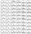 |
Fig. B.1 Observed spectra of Fe XXVI 1.778 Å, Fe XXV 1.859 Å, Ca XX 3.018 Å, Ar XVIII 3.731 Å, S XVI 4.734 Å and Si XIV 6.184 Å are shown in vertical columns from left to right. Each column presents spectra at ten orbital phases from 0.05 (top) to 0.95 (bottom). The x-axis represents the velocity shift from the line wavelength (in units of 1000 km/s), while the y-axis shows the observed flux (photons/s/keV/cm2 on Earth) with error bars and the model-fit (solid line) |
References
- Antokhin, I. I., & Cherepashchuk, A. M. 2019, ApJ, 871, 244 [Google Scholar]
- Antokhin, I. I., Cherepashchuk, A. M., Antokhina, E. A., & Tatarnikov, A. M. 2022, ApJ, 926, 123 [NASA ADS] [CrossRef] [Google Scholar]
- Dubus, G., Cerutti, B., & Henri, G. 2010, MNRAS, 404, L55 [NASA ADS] [Google Scholar]
- Giacconi, R., Gorenstein, P., Gursky, H., & Waters, J. R. 1967, Astrophys. J., 148, L119 [Google Scholar]
- Hanson, M. M., Still, M. D., & Fender, R. P. 2000, ApJ, 541, 308 [Google Scholar]
- Hjalmarsdotter, L., Zdziarski, A. A., Larsson, S., et al. 2008, MNRAS, 384, 278 [NASA ADS] [CrossRef] [Google Scholar]
- Kallman, T., McCollough, M., Koljonen, K., et al. 2019, ApJ, 874, 51 [NASA ADS] [CrossRef] [Google Scholar]
- Koljonen, K. I. I., & Maccarone, T. J. 2017, MNRAS, 472, 2181 [NASA ADS] [CrossRef] [Google Scholar]
- Koljonen, K. I. I., Hannikainen, D. C., McCollough, M. L., Pooley, G. G., & Trushkin, S. A. 2010, MNRAS, 406, 307 [NASA ADS] [CrossRef] [Google Scholar]
- Koljonen, K. I. I., Maccarone, T., McCollough, M. L., et al. 2018, A&A, 612, A27 [NASA ADS] [CrossRef] [EDP Sciences] [Google Scholar]
- Lommen, D., Yungelson, L., van den Heuvel, E., Nelemans, G., & Portegies Zwart, S. 2005, A&A, 443, 231 [NASA ADS] [CrossRef] [EDP Sciences] [Google Scholar]
- Parsignault, D. R., Gursky, H., Kellogg, E. M., et al. 1972, Nat. Phys. Sci., 239, 123 [Google Scholar]
- Suryanarayanan, A., Paerels, F., & Leutenegger, M. 2024, ApJ, 969, 110 [Google Scholar]
- Szostek, A., & Zdziarski, A. A. 2008, MNRAS, 386, 593 [Google Scholar]
- van Kerkwijk, M. H., Geballe, T. R., King, D. L., van der Klis, M., & van Paradijs, J. 1996, A&A, 314, 521 [Google Scholar]
- Veledina, A., Muleri, F., Poutanen, J., et al. 2024a, Nat. Astron., 8, 1031 [NASA ADS] [CrossRef] [Google Scholar]
- Veledina, A., Poutanen, J., Bocharova, A., et al. 2024b, A&A, 688, L27 [NASA ADS] [CrossRef] [EDP Sciences] [Google Scholar]
- Vilhu, O., Hjalmarsdotter, L., Zdziarski, A., et al. 2003, A&A, 411, L405 [NASA ADS] [CrossRef] [EDP Sciences] [Google Scholar]
- Vilhu, O., Hakala, P., Hannikainen, D. C., McCollough, M., & Koljonen, K. 2009, A&A, 501, 679 [NASA ADS] [CrossRef] [EDP Sciences] [Google Scholar]
- Vilhu, O., & Hannikainen, D. C. 2013, A&A, 550, A48 [NASA ADS] [CrossRef] [EDP Sciences] [Google Scholar]
- Vilhu, O., Kallman, T. R., Koljonen, K. I. I., & Hannikainen, D. C. 2021, A&A, 649, A176 [NASA ADS] [CrossRef] [EDP Sciences] [Google Scholar]
- Vilhu, O., Koljonen, K. I. I., & Hannikainen, D. C. 2023, A&A, 674, A74 [NASA ADS] [CrossRef] [EDP Sciences] [Google Scholar]
- Waltman, E. B., Fiedler, R. L., Johnston, K. J., & Ghigo, F. D. 1994, AJ, 108, 179 [Google Scholar]
- Waltman, E. B., Foster, R. S., Pooley, G. G., Fender, R. P., & Ghigo, F. D. 1996, AJ, 112, 2690 [NASA ADS] [CrossRef] [Google Scholar]
- XRISM Collaboration (Audard, M., et al.) 2024, ApJ, 977, L34 [Google Scholar]
- Zdziarski, A. A., Maitra, C., Frankowski, A., Skinner, G. K., & Misra, R. 2012, MNRAS, 426, 1031 [Google Scholar]
- Zdziarski, A. A., Mikolajewska, J., & Belczynski, K. 2013, MNRAS, 429, L104 [Google Scholar]
Written by Craig Markward.
All Tables
Results of the fitting procedures using a sine-curve for radial velocities and two absorbers for line intensities.
All Figures
|
Fig. 1 Chandra/HEG spectrum (OBSID 7268). The lines we analysed are marked. The flux (F) is in units of photons/s/keV/cm2 at Earth. |
| In the text | |
|
Fig. 2 Sine curve fits for the radial velocity (km/s, left panels) and two-absorber fits for the line emission (scaled, photons/s, right panels) for the six analysed emission lines. The dashed line represents the continuum at the line. |
| In the text | |
|
Fig. 3 K-amplitude (upper-left), the orbital phase with the highest blueshift (upper-right), Awind (lower left), and Aclump (lower right) as a function of the ionisation potential of the ion. Dots with error bars show the emission lines, while the filled boxes indicate the continua at the lines. ‘Si2G’ in the upper panels denotes the P Cygni (two-Gaussian) solution for the Si XIV line. |
| In the text | |
|
Fig. 4 Top panel: K-amplitudes of grid points plotted against their y-values sorted by their x-values. Middle panel: same as the upper panel but for the orbital phases with the highest blueshift. The values corresponding to the observed emission lines are marked by horizontal lines. Bottom panel: line formation sites combining information from the two upper panels (dots with error bars). The bottom panel also shows (dotted) curved contours with constant K-values (200, 300, 400, and 500 km/s increasing from the WR surface) and radial (dotted) contours with the constant bluest phases ϕ (from 0.3 to 0.7). |
| In the text | |
|
Fig. 5 Alternative arrangement for the emission regions of the Si XIV, S XVI, Ar XVIII, and Ca XX lines. Parts of the Ca and Ar lines formed in the compact star disc or corona (see the text). The solid curves represent surfaces with a constant ionisation parameter marked by a log ξ-value. These curves are intersections with the (x,y) plane of 3D surfaces where the lines are expected to form. For clarity, the error bars have been shifted vertically from y=0. The coordinate system is the same as in Fig. 4. |
| In the text | |
|
Fig. A.1 Permitted (Θj, ϕj) range corresponding to the angle between the line of sight and the jet (or funnel) axis to lie between 26–28 degrees. The dots indicate constraints on the inclination between 20–60 degrees, while the plus signs (darker region) mark the range between 26–28 degrees. The star represents the jet parameter values given by Dubus et al. (2010). |
| In the text | |
|
Fig. B.1 Observed spectra of Fe XXVI 1.778 Å, Fe XXV 1.859 Å, Ca XX 3.018 Å, Ar XVIII 3.731 Å, S XVI 4.734 Å and Si XIV 6.184 Å are shown in vertical columns from left to right. Each column presents spectra at ten orbital phases from 0.05 (top) to 0.95 (bottom). The x-axis represents the velocity shift from the line wavelength (in units of 1000 km/s), while the y-axis shows the observed flux (photons/s/keV/cm2 on Earth) with error bars and the model-fit (solid line) |
| In the text | |
Current usage metrics show cumulative count of Article Views (full-text article views including HTML views, PDF and ePub downloads, according to the available data) and Abstracts Views on Vision4Press platform.
Data correspond to usage on the plateform after 2015. The current usage metrics is available 48-96 hours after online publication and is updated daily on week days.
Initial download of the metrics may take a while.