| Issue |
A&A
Volume 688, August 2024
|
|
|---|---|---|
| Article Number | L27 | |
| Number of page(s) | 8 | |
| Section | Letters to the Editor | |
| DOI | https://doi.org/10.1051/0004-6361/202451356 | |
| Published online | 14 August 2024 | |
Ultrasoft state of microquasar Cygnus X-3: X-ray polarimetry reveals the geometry of the astronomical puzzle
1
Department of Physics and Astronomy, FI-20014 University of Turku, Finland
2
Nordita, KTH Royal Institute of Technology and Stockholm University, Hannes Alfvéns väg 12, SE-10691 Stockholm, Sweden
3
INAF Istituto di Astrofisica e Planetologia Spaziali, Via del Fosso del Cavaliere 100, 00133 Roma, Italy
4
Dipartimento di Fisica, Università degli Studi di Roma “Tor Vergata”, Via della Ricerca Scientifica 1, 00133 Roma, Italy
5
Dipartimento di Fisica, Università degli Studi di Roma “La Sapienza”, Piazzale Aldo Moro 5, 00185 Roma, Italy
6
Astronomical Institute of the Czech Academy of Sciences, Boční II 1401/1, 14100 Praha 4, Czech Republic
7
Nicolaus Copernicus Astronomical Center, Polish Academy of Sciences, Bartycka 18, 00-716 Warszawa, Poland
8
Astrophysics Group, Cavendish Laboratory, 19 J. J. Thomson Avenue, Cambridge CB3 0HE, UK
9
Harvard-Smithsonian Center for Astrophysics, 60 Garden St, Cambridge, MA 02138, USA
10
Astrophysics, Department of Physics, University of Oxford, Denys Wilkinson Building, Keble Road, Oxford OX1 3RH, UK
11
Dipartimento di Matematica e Fisica, Università degli Studi Roma Tre, Via della Vasca Navale 84, 00146 Roma, Italy
12
Max Planck Institute for Astrophysics, Karl-Schwarzschild-Str 1, 85741 Garching, Germany
13
Space Research Institute, Russian Academy of Sciences, Profsoyuznaya 84/32, 117997 Moscow, Russia
Received:
2
July
2024
Accepted:
30
July
2024
Abstract
Cygnus X-3 is an enigmatic X-ray binary that is both an exceptional accreting system and a cornerstone for population synthesis studies. Prominent X-ray and radio properties follow a well-defined pattern, and yet the physical reasons for the state changes observed in this system are not known. Recently, the presence of an optically thick envelope around the central source in the hard state was revealed using the X-ray polarization data obtained with the Imaging X-ray Polarimetry Explorer (IXPE). In this work we analyse IXPE data obtained in the ultrasoft (radio quenched) state of the source. The average polarization degree (PD) of 11.9 ± 0.5% at a polarization angle (PA) of 94° ±1° is inconsistent with the simple geometry of the accretion disc viewed at an intermediate inclination. The high PD, the blackbody-like spectrum, and the weakness of fluorescent iron line imply that the central source is hidden behind the optically thick outflow, similar to the hard-state geometry, and its beamed radiation is scattered, by the matter located along the funnel axis, towards our line of sight. In this picture the observed PD is directly related to the source inclination, which we conservatively determine to lie in the range 26° < i < 28°. Using the new polarimetric properties, we propose a scenario that can be responsible for the cyclic behaviour of the state changes in the binary.
Key words: accretion, accretion disks / polarization / stars: black holes / X-rays: binaries / X-rays: individuals: Cyg X-3
Corresponding author; This email address is being protected from spambots. You need JavaScript enabled to view it. .
© The Authors 2024
 Open Access article, published by EDP Sciences, under the terms of the Creative Commons Attribution License (https://creativecommons.org/licenses/by/4.0), which permits unrestricted use, distribution, and reproduction in any medium, provided the original work is properly cited.
This article is published in open access under the Subscribe to Open model. This email address is being protected from spambots. You need JavaScript enabled to view it. to support open access publication.
1. Introduction
Accreting binary system Cygnus X-3 (hereafter Cyg X-3) is one of the first detected X-ray sources (Giacconi et al. 1967). This persistent source shows several exceptional observational properties. It is the brightest X-ray binary in radio wavelengths, with fluxes that can reach 20 Jy (McCollough et al. 1999; Corbel et al. 2012), and is one of a few Galactic binaries with detectable γ-ray emission (Tavani et al. 2009; Atwood et al. 2009). It is one of the shortest-period X-ray binaries, Porb = 4.8 h, that is also rapidly changing owing to the high mass-loss rate from the system (van der Klis & Bonnet-Bidaud 1981; Antokhin & Cherepashchuk 2019). The short period implies that the luminous companion star is very compact, suggesting that the donor is a Wolf-Rayet (WR) star, which is further supported by the hydrogen-depleted infrared spectrum (van Kerkwijk et al. 1992, 1996; Fender et al. 1999). This unique binary plays an important role in population synthesis studies: a successful model is obliged to reproduce the presence of Cyg X-3 in the Milky Way, the compact object in a tight binary orbit with the WR companion; at the same time, current estimates suggest the presence of only one such system in our Galaxy (Lommen et al. 2005).
There is no detected optical counterpart due to the considerable distance to the source (D = 9.7 ± 0.5 kpc; Reid & Miller-Jones 2023) and its location close to the Galactic plane resulting in high absorption along to the line of sight. However, the orbital phase dependence of radio, infrared, X-ray, and γ-ray properties of the system have been studied extensively (e.g. McCollough et al. 1999; Fender et al. 1999; Zdziarski et al. 2018). The source was found to regularly switch between several spectral states characterised by distinct X-ray and radio properties (Fig. 1 and Szostek et al. 2008; Koljonen et al. 2010). Transitions between the spectral states are generally thought to be related to the changes in accretion geometry in the system, but the exact picture of plasma configuration and understanding of the physical reasons for these changes are still missing. This makes the source an ideal target for X-ray polarimetric studies.
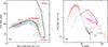 |
Fig. 1. Spectral states of Cyg X-3. Panel a: Radio–X-ray track made by Cyg X-3 as it swings between different spectral states (data from Zdziarski et al. 2016). Panel b: Set of average broadband spectra corresponding to the hard/radio quiescent (blue), intermediate/minor flaring (orange), ultrasoft/radio quenched (black), and soft non-thermal/flaring (magenta) states, as introduced in Szostek et al. (2008). IXPE data are shown with red symbols and the 2σ upper limit at 30 keV (in red) is from Swift/BAT. |
The source is most often found in the hard X-ray quiescent radio state (Waltman et al. 1996; Hjalmarsdotter et al. 2009), when the X-ray continuum can be roughly described as a cutoff power law with a peak at around 20 keV (Fig. 1b), and prominent iron lines can be clearly identified. Spectral decomposition in this state is complicated by the unknown absorption, in particular its component that is intrinsic to the source (Hjalmarsdotter et al. 2008; Zdziarski et al. 2010).
Cyg X-3 is found to make regular transitions towards the (ultra-)soft state, when the hard X-ray flux drops dramatically and the spectrum resembles a blackbody with kTbb ≈ 1.5 keV. Radio fluxes are likewise suppressed, motivating the name of the radio quenched state. This transition is often followed by a major radio flare, when the highest radio fluxes are detected, while the X-ray continuum is moderately soft and exhibits a high-energy tail (Szostek et al. 2008; Koljonen et al. 2010).
Exceptional multiwavelength properties of the source and a fast, repeating swing between different states prompted Hjellming (1973) to call it ‘an astronomical puzzle’. Interest in solving this puzzle has persisted for more than 50 years. A new chapter in the study of the source has been opened with the launch of the Imaging X-ray Polarimetry Explorer (IXPE), which enabled the first X-ray polarization studies in the 2−8 keV band.
The source was previously observed by IXPE in the X-ray hard (radio quiescent) and intermediate (minor flaring) states (Veledina et al. 2024). The first X-ray polarimetric observations in October–November 2022 revealed a high average polarization degree (PD) of 20.6 ± 0.3% (which changed to 23% after accounting for the unpolarized contribution of the iron line). The polarization angle, PA =  , suggests that it is nearly orthogonal to the extended jet emission and relativistic ejections observed in the system. The spectropolarimetric properties suggest that the X-ray emission is produced solely by reflection, indicating the presence of obscuring material hiding the central engine from the observer’s line of sight. The apparent high luminosity of 1038 erg s−1 and a much higher luminosity emitted along the funnel in the obscuring outflow (> 5.5 × 1039 erg s−1) imply that Cyg X-3 belongs to the class of ultraluminous X-ray sources. The dramatic drop in polarization in the minor flaring state, PD = 10.0 ± 0.5%, was interpreted in terms of the dilution of the outflow.
In this picture, the outflow could disappear completely in the ultrasoft and soft non-thermal states (radio quenched and major flaring states, respectively). Here we present the X-ray polarimetric properties of Cyg X-3 in the ultrasoft state, with the aim of verifying the source accretion geometry and of understanding the physical reasons of state transitions.
2. Data
IXPE observed the source in the ultrasoft state on 2024 June 2−3. We followed the standard data analysis procedures that are described in detail in Appendix A. Further analysis will be presented in an upcoming work (Rodriguez Cavero et al., in prep.). We used simultaneous Swift/BAT data1 (Gehrels et al. 2004) to estimate the flux in the hard X-ray band. We also monitored the source in radio with the AMI telescope at 15 GHz. The results of the radio monitoring of Cyg X-3 are presented in Appendix B.
3. Results
The source was observed in the ultrasoft X-ray spectral state (Fig. 1b), with highly suppressed hard X-ray flux, as indicated by Swift/BAT. We note the lower flux, with respect to its typical value (Szostek et al. 2008), around the iron line complex (compare the black and red spectra). Radio fluxes were likewise historically low, 4.5 ± 0.3 mJy (Fig. 1a and Appendix B). The average polarimetric properties are shown in Fig. 2. We find average PD = 11.9 ± 0.5% and PA = 94° ±1° and no significant energy dependence, in particular, around the iron line range. The PA is shifted by ∼4° with respect to the values detected in the hard and intermediate states.
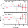 |
Fig. 2. Average PD and PA as a function of energy. The horizontal dashed lines correspond to the energy-average values. |
Spectropolarimetric data suggest an absence of the prominent iron line, in contrast to the hard and intermediate states (see Appendix A). The spectrum in this state was previously well fit by a single blackbody component, a multicolour disc, or a low-temperature Comptonization component (Szostek et al. 2008; Hjalmarsdotter et al. 2009; Koljonen et al. 2018). However, high PD and its independence of energy is not consistent with either of the aforementioned components.
Next we consider variations of polarimetric properties. Prominent orbital flux variations are detected, with the typical profile shape of a brief dip and a more extended peak (Fig. 3a). In Figs. 3b, c we show the PD and PA averaged over different orbital cycles. In contrast to the hard state, we find pronounced changes of PD in the ultrasoft state. The PA remains constant within the errors, yet systematically shifted with respect to the hard- and intermediate-state data in all bins. We compared the spectropolarimetric properties of time bins 2 and 3 (in Fig. 3b, c) to those of time bin 5 (see Figs. A.3 and A.4). The iron line is detected in time bin 5, albeit at a low significance; for the combined bin 2+3 its contribution is compatible with zero.
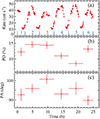 |
Fig. 3. Time variations of the IXPE count rate in the 2−8 keV band and the orbit-average PD and PA. Time is measured from the beginning of the observation at MJD 60463.8124. Boundaries of the time bins (except the beginning and end of the observation) correspond to the orbital phase 0. |
Previous IXPE observations in the hard and intermediate states revealed significant variations of polarization at the orbital period. In Fig. 4 we show the orbital phase-resolved polarimetric properties of the source in the three observed states. The PD variations in the ultrasoft state are nearly identical to those found in the intermediate state, but the PA shows a pronounced peak around phase 0 (corresponding to the lowest X-ray fluxes). Using the pcube analysis of the 2−5 keV and 5−8 keV energy bins, we also checked whether the energy dependence of PD is different for these two orbital phases. We find no difference between the two energy bins for the high X-ray flux spectra, associated with phase 0.5, but for the low-flux bin (phase 0) the PD decreases with energy at the 90% confidence level. We also performed orbital phase-resolved spectropolarimetry (see Figs. A.1 and A.2). The iron line is detected in the spectra around phase 0; for phase 0.5 only an upper limit can be determined (see Appendix A).
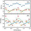 |
Fig. 4. Orbital phase dependence of the PD and PA from the hard state (blue triangles), the intermediate state (orange open squares), and ultrasoft state (red circles). The green lines show the best-fit rotating vector model (Appendix C) to the ultrasoft-state data. |
4. Discussion
Previous IXPE studies clearly showed that the states of Cyg X-3 do not simply match the hard or intermediate states of other X-ray binaries, and the standard scenarios that have been confirmed, for example Swift J1727.8−1613 (Veledina et al. 2023; Ingram et al. 2024; Podgorný et al. 2024) and Cyg X-1 (Krawczynski et al. 2022) cannot be applied to this source. If the soft state of Cyg X-3 is analogous to the other soft-state sources, the PD ∼ 1−2% can be expected (comparable to the measurements of Cyg X-1 and Swift J1727.8−1613 that are thought to have similar orbital inclinations; Svoboda et al. 2024; Steiner et al. 2024). On the contrary, we observe the average PD ≈ 12%, that appears somewhat higher than that observed in the intermediate state. This puts tight constraints on radiative mechanisms relevant to this state of the system, as well as the accretion geometry.
A high PD that is independent of energy is in line with the single reflection or scattering scenario. The presence of an obscuring medium covering the central source along the line of sight is inevitable for the production of the high polarization. The absence of a clear contribution of the iron line, both in spectral and polarimetric properties, indicates the spectrum is not dominated by the reflection off the cold and dense matter, suggested for the hard state (Veledina et al. 2024). This conclusion is supported by the previous spectroscopic analysis of the Chandra data (Kallman et al. 2019), that found an absence of the fluorescent line from neutral iron; however, lines of the highly ionised species of Fe XXV and Fe XXVI, whose motion is associated with the compact object (Vilhu et al. 2009) remain prominent throughout the ultrasoft state.
We have tested various scenarios where the observed polarization arises from the reflection at the inner walls of the funnel (using the same setup described in Podgorný et al. 2022, 2023; Veledina et al. 2024). We considered the orbital inclination in the range 20° < i < 40°, in line with previous estimates (Vilhu et al. 2009; Antokhin et al. 2022), and varied the density and ionisation of the medium. When decreasing the density of the funnel walls (with respect to the hard state NH = 1024 cm−2), the PD becomes a decreasing function of energy in the IXPE range because the matter becomes effectively transparent to high-energy radiation. Hence, the overall smaller funnel density cannot be responsible for the observed changes of polarization.
We also considered cases of higher ionisation. With increasing ionisation, we generally observe the decrease in the overall PD owing to the enhanced role of multiple scatterings. We find that in order to reproduce the lack of neutral and/or moderately ionized iron lines, the ionisation parameter (giving the ratio of ionising flux to the number density of matter) ξ ≳ 5000 is required. This value is somewhat high, yet still within the boundaries of the allowed range 2 ≲ log ξ ≲ 4 coming from the line spectroscopy (Kallman et al. 2019). However, at these high values the multiple scatterings occur within a large fraction of the envelope, similar to a spherical shell, hence the PD drops to 1%, becoming inconsistent with the observed levels. We conclude that the increased ionization of the entire funnel cannot produce the observed high and energy-independent PD. On the other hand, transmission of the polarized light (reflected from the funnel surface) through the ionized medium may lead to the observed ultrasoft-state polarization properties.
The observed blackbody-like spectrum and PD = 10−15% naturally appear in the scenario where the intrinsic radiation undergoes single Thomson scattering in the medium along the axis of the optically thick funnel and the observer sees only this scattered component (see Fig. 5). In this case, the observed average PD gives the direct estimate on the inclination. For the single Thomson scattering regime we have
 (1)
(1)
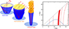 |
Fig. 5. Accretion geometry and parameters of Cyg X-3. Left: Sketch of the geometry associated with the hard, intermediate, and ultrasoft states. The red arrows indicate the direction of the incident and reflected or scattered photons by the optically thick outflow (blue). In the hard state, the only photons reflected at the back surface of the funnel are visible to the observer, while in the intermediate state the reflected and scattered emission is coming from different sides of the funnel (the funnel upper parts become semi-transparent or clumpy). In the soft state, radiation scattered off the matter lying along the funnel axis dominates over the contribution of reflected emission. Right: Polarization of radiation undergoing single scattering above a funnel of half-opening angle α for different observer inclinations i (red lines). The filled red band depicts the conservative PD range 10.8−12.4% of Cyg X-3 in the ultrasoft state, which translates to the inclination of i = 26° −28°; this is very close to the values of |
where μ is the cosine of the scattering angle. Thus PD = 11.9 ± 0.5% translates to inclination ![Mathematical equation: $ i=\arccos[(1-P)/(1+P)]^{1/2}=27{{\overset{\circ}{.}}}5\pm 0{{\overset{\circ}{.}}}5 $](/articles/aa/full_html/2024/08/aa51356-24/aa51356-24-eq4.gif) . This constraint is relevant to the geometry of an infinitely narrow funnel. Calculations that include averaging over the non-zero opening angle α of a conical funnel, for an isotropic central source and equal scattering probability within the funnel, show that PD dependence on α is weak (see nearly vertical contours of constant PD in Fig. 5).
. This constraint is relevant to the geometry of an infinitely narrow funnel. Calculations that include averaging over the non-zero opening angle α of a conical funnel, for an isotropic central source and equal scattering probability within the funnel, show that PD dependence on α is weak (see nearly vertical contours of constant PD in Fig. 5).
Orbital variability can be used as an independent tracer of accretion geometry. Orbital profiles of gamma-ray fluxes were previously explained by a jet-orbital axis misalignment (Dubus et al. 2010; Zdziarski et al. 2018) or bending of the jet or funnel (Dmytriiev et al. 2024). Radio fluxes were likewise varying due to changing wind absorption (Zdziarski et al. 2018). Interestingly though, we find an absence of the orbital modulation of radio fluxes during IXPE observations (Fig. B.2 in Appendix B). Polarization properties of the precessing funnel can be tested using the rotating vector model (see Appendix C; Radhakrishnan & Cooke 1969; Poutanen 2020). We note that this model does not necessarily assume that the radiation beam collimated by the funnel is precessing, but there could be an asymmetry in the distribution of scattering material, for example, formed by the bow shock (Antokhin et al. 2022) with the geometry fixed in the corotating frame of the binary. In Fig. 4 we show the best-fit model (green line). The fit gives χ2/d.o.f. = 25.7/8. The model fails to reproduce the data because the amplitude of PA variations in excess of 20° translates to the changes in PD, predicted by this model for i = 27°, by about 9%, much larger than the observed PD amplitude. While the model can reproduce orbital variations of PA, the precessing funnel scenario cannot be responsible for the orbital changes of PD. This may be related to a more complex dependence of PD on the angle between the funnel axis and the line of sight.
We note that the orbital-average ultrasoft-state PD shows pronounced variations from one orbital cycle to another (Fig. 3). The changes could indicate secular variations of funnel parameters, but might as well be related to the switching between the dominating mechanisms responsible for the polarization production: reflection at the funnel walls and scattering within and/or on top of the funnel itself. The latter possibility can be verified by comparing the spectra corresponding to different polarization levels: those coming from the scattering are expected to have no pronounced neutral iron line. In our case, however, the normalisation of the line in time bin 5 and an upper limit in combined time bin 2+3 are comparable. Thus, we cannot conclusively confirm or rule out this possibility.
Time variations of PD may potentially be linked to the changes in the optical depth of the scattering material: higher Thomson optical depth τ leads to higher scattered fluxes. Higher τ also leads to the reduction of PD, as per the increased role of the (unpolarized) contribution of higher-order scatterings. Changes of τ may be the reason for the visible anti-correlation between the orbital fluence and measured PD (see Fig. 3). The PD drop by a factor of 1.5 between the time bins 2+3 and 5 corresponds to the transition from an optically thin medium (τ < < 1) to the medium of Thomson optical depth τ ≈ 0.35. We can then obtain the average bolometric luminosity of the system using the ultrasoft-state flux estimate from Hjalmarsdotter et al. (2009) (with updated distance estimate and when accounting for the scattered fraction corresponding to τ = 0.35). We obtain the intrinsic luminosity estimate Lint ≈ 1.4 × 1039 erg s−1. This estimate is close to the Eddington limit for He-rich material if the compact object has mass ≲5 solar masses, in line with previous results (Zdziarski et al. 2013; Koljonen & Maccarone 2017).
At the same time, the spectra corresponding to the high flux phases (orbital phase 0.5) show strong suppression of the iron line compared to the low flux phases (phase 0, see Appendix A). This may indicate systematic changes between scattering (phase 0.5) and reflection (phase 0) mechanisms at different orbital phases, attributed to the changing viewing angle of precessing funnel. The observed high-flux PD = 11.2 ± 0.4% corresponds to the scattering angle (inclination) in this phase  .
.
The polarimetric properties discussed above imply that during the ultrasoft state, when the jet is quenched, the funnel interior and the channel above it become filled with matter coming from the WR wind and perhaps from the inner walls of the outflow (this picture is similar to the jet cocoon scenario, Koljonen et al. 2018). The amount of material along the funnel axis in this state is much larger than in the hard state when the powerful jet cleared the material within the funnel beam (and further away above it) and the observer saw only the light reflected from the inner walls. The drop in polarization during the intermediate (minor flaring) state might then be explained by the accumulation of matter close at the inner boundaries of the funnel and replacement of the reflection at the sharp inner boundary by the reflection within the volume close to this boundary (see Fig. 5). The effects of matter ionisation may also play a role in the PD reduction; in this case the funnel becomes partially transparent to the reflected radiation (but not the incident radiation).
We suggest the physical reason for the spectral changes Cyg X-3 and correlated radio activity of the source is solely related to the amount of material within the optically thick envelope of the source. In the hard state the amount of matter along the funnel axis is low and the spectrum is produced by the reflection off nearly neutral material of the funnel walls. A radio jet operates effectively within the funnel and produces a stable level of radio emission. The transition towards the soft state may be related to the accumulation of matter in the interior of the funnel, causing a reduction of the characteristic reflection (scattering) angle. It may also cause the intermittent character of radio emission (minor flaring). In the ultrasoft state, the observed radiation is caused by the Thomson scattering of the incident spectrum by the optically thin medium located along the funnel axis. Radio quenching is likewise related to the presence of a substantial amount of matter within the funnel, which is then wiped away during the transition to the soft non-thermal state, causing major radio flares. Once the matter along the funnel axis is cleared away by the jet, the source is observed again in the hard X-ray, quiescent radio state.
5. Summary
We have studied the X-ray polarimetric properties of the X-ray binary Cyg X-3 during the ultrasoft state. The high PD = 11.9 ± 0.5% and PA = 94° ±1° indicate that the central source is covered by a thick envelope, similar to the previously observed hard and intermediate states. The polarization of the continuum radiation can arise from a single scattering off the optically thin medium located along the funnel axis. This is different from the scenario for the other states, where the X-ray continuum is dominated by the reflection from funnel walls.
We showed that the PD in this case can serve as a direct probe of the orbital inclination,  . We discussed the changes in the orbit-average and phase-dependent PDs and find that this scenario can be realised in the phases with highest flux, with PD = 11.2 ± 0.4%, leading to the conservative inclination estimate 26° < i < 28°.
Changes of the orbital-average PD may be related to the optical depth variations of scattering matter. The transition between the hard and ultrasoft states may in turn be caused by the filling of the funnel by the matter (coming either from the funnel walls or from the enhanced WR wind) linked to the jet quenching. The major flaring state can then be related to the ejection of matter from the funnel, its eventual emptying, and the transition of the source to the hard state. This closes the loop of the correlated radio and X-ray activity in Cyg X-3.
Acknowledgments
The Imaging X-ray Polarimetry Explorer (IXPE) is a joint US and Italian mission. The US contribution is supported by the National Aeronautics and Space Administration (NASA) and led and managed by its Marshall Space Flight Center (MSFC), with industry partner Ball Aerospace (contract NNM15AA18C). The Italian contribution is supported by the Italian Space Agency (Agenzia Spaziale Italiana, ASI) through contract ASI-OHBI-2022-13-I.0, agreements ASI-INAF-2022-19-HH.0 and ASI-INFN-2017.13-H0, and its Space Science Data Center (SSDC) with agreements ASI-INAF-2022-14-HH.0 and ASI-INFN 2021-43-HH.0, and by the Istituto Nazionale di Astrofisica (INAF) and the Istituto Nazionale di Fisica Nucleare (INFN) in Italy. This research used data products provided by the IXPE Team (MSFC, SSDC, INAF, and INFN) and distributed with additional software tools by the High-Energy Astrophysics Science Archive Research Center (HEASARC), at NASA Goddard Space Flight Center (GSFC). This research has been supported by the Academy of Finland grant 355672 (AV, VA) and the Vilho, Yrjö, and Kalle Väisälä foundation (SVF). ADM, FLM, EC, FM and PS are partially supported by MAECI with grant CN24GR08 “GRBAXP: Guangxi-Rome Bilateral Agreement for X-ray Polarimetry in Astrophysics”. AAZ acknowledges support from the Polish National Science Center grants 2019/35/B/ST9/03944, 2023/48/Q/ST9/00138, and from the Copernicus Academy grant CBMK/01/24. JPod and MD acknowledge the support from the Czech Science Foundation project GACR 21–06825X and the institutional support from the Astronomical Institute RVO:6798581. DG and LR thank the staff of Lord’s Bridge, Cambridge, for their support in making the AMI observations.
References
- Antokhin, I. I., & Cherepashchuk, A. M. 2019, ApJ, 871, 244 [Google Scholar]
- Antokhin, I. I., Cherepashchuk, A. M., Antokhina, E. A., & Tatarnikov, A. M. 2022, ApJ, 926, 123 [NASA ADS] [CrossRef] [Google Scholar]
- Arnaud, K. A. 1996, ASP Conf. Ser., 101, 17 [Google Scholar]
- Atwood, W. B., Abdo, A. A., Ackermann, M., et al. 2009, ApJ, 697, 1071 [CrossRef] [Google Scholar]
- Baldini, L., Barbanera, M., Bellazzini, R., et al. 2021, Astropart. Phys., 133, 102628 [NASA ADS] [CrossRef] [Google Scholar]
- Baldini, L., Bucciantini, N., Di Lalla, N., et al. 2022, SoftwareX, 19, 101194 [NASA ADS] [CrossRef] [Google Scholar]
- Corbel, S., Dubus, G., Tomsick, J. A., et al. 2012, MNRAS, 421, 2947 [CrossRef] [Google Scholar]
- Di Marco, A., Costa, E., Muleri, F., et al. 2022, AJ, 163, 170 [NASA ADS] [CrossRef] [Google Scholar]
- Di Marco, A., Soffitta, P., Costa, E., et al. 2023, AJ, 165, 143 [CrossRef] [Google Scholar]
- Dmytriiev, A., Zdziarski, A. A., Malyshev, D., Bosch-Ramon, V., & Chernyakova, M. 2024, ApJ, submitted [arXiv:2405.09154] [Google Scholar]
- Dubus, G., Cerutti, B., & Henri, G. 2010, MNRAS, 404, L55 [NASA ADS] [Google Scholar]
- Fender, R. P., Hanson, M. M., & Pooley, G. G. 1999, MNRAS, 308, 473 [NASA ADS] [CrossRef] [Google Scholar]
- Gehrels, N., Chincarini, G., Giommi, P., et al. 2004, ApJ, 611, 1005 [Google Scholar]
- Giacconi, R., Gorenstein, P., Gursky, H., & Waters, J. R. 1967, ApJ, 148, L119 [NASA ADS] [CrossRef] [Google Scholar]
- Hickish, J., Razavi-Ghods, N., Perrott, Y. C., et al. 2018, MNRAS, 475, 5677 [NASA ADS] [CrossRef] [Google Scholar]
- Hjalmarsdotter, L., Zdziarski, A. A., Larsson, S., et al. 2008, MNRAS, 384, 278 [NASA ADS] [CrossRef] [Google Scholar]
- Hjalmarsdotter, L., Zdziarski, A. A., Szostek, A., & Hannikainen, D. C. 2009, MNRAS, 392, 251 [NASA ADS] [CrossRef] [Google Scholar]
- Hjellming, R. M. 1973, Science, 182, 1089 [CrossRef] [Google Scholar]
- Ingram, A., Bollemeijer, N., Veledina, A., et al. 2024, ApJ, 968, 76 [NASA ADS] [CrossRef] [Google Scholar]
- Kallman, T., McCollough, M., Koljonen, K., et al. 2019, ApJ, 874, 51 [NASA ADS] [CrossRef] [Google Scholar]
- Kislat, F., Clark, B., Beilicke, M., & Krawczynski, H. 2015, Astropart. Phys., 68, 45 [NASA ADS] [CrossRef] [Google Scholar]
- Koljonen, K. I. I., & Maccarone, T. J. 2017, MNRAS, 472, 2181 [NASA ADS] [CrossRef] [Google Scholar]
- Koljonen, K. I. I., Hannikainen, D. C., McCollough, M. L., Pooley, G. G., & Trushkin, S. A. 2010, MNRAS, 406, 307 [NASA ADS] [CrossRef] [Google Scholar]
- Koljonen, K. I. I., Maccarone, T., McCollough, M. L., et al. 2018, A&A, 612, A27 [NASA ADS] [CrossRef] [EDP Sciences] [Google Scholar]
- Krawczynski, H., Muleri, F., Dovčiak, M., et al. 2022, Science, 378, 650 [NASA ADS] [CrossRef] [Google Scholar]
- Lommen, D., Yungelson, L., van den Heuvel, E., Nelemans, G., & Portegies Zwart, S. 2005, A&A, 443, 231 [NASA ADS] [CrossRef] [EDP Sciences] [Google Scholar]
- McCollough, M. L., Robinson, C. R., Zhang, S. N., et al. 1999, ApJ, 517, 951 [NASA ADS] [CrossRef] [Google Scholar]
- Perrott, Y. C., Scaife, A. M. M., Green, D. A., et al. 2013, MNRAS, 429, 3330 [NASA ADS] [CrossRef] [Google Scholar]
- Podgorný, J., Dovčiak, M., Marin, F., Goosmann, R., & Różańska, A. 2022, MNRAS, 510, 4723 [CrossRef] [Google Scholar]
- Podgorný, J., Marin, F., & Dovčiak, M. 2023, MNRAS, 526, 4929 [CrossRef] [Google Scholar]
- Podgorný, J., Svoboda, J., Dovčiak, M., et al. 2024, A&A, 686, L12 [NASA ADS] [CrossRef] [EDP Sciences] [Google Scholar]
- Poutanen, J. 2020, A&A, 641, A166 [NASA ADS] [CrossRef] [EDP Sciences] [Google Scholar]
- Radhakrishnan, V., & Cooke, D. J. 1969, Astrophys. Lett., 3, 225 [NASA ADS] [Google Scholar]
- Reid, M. J., & Miller-Jones, J. C. A. 2023, ApJ, 959, 85 [CrossRef] [Google Scholar]
- Soffitta, P., Baldini, L., Bellazzini, R., et al. 2021, AJ, 162, 208 [CrossRef] [Google Scholar]
- Steiner, J. F., Nathan, E., Hu, K., et al. 2024, ApJ, 969, L30 [NASA ADS] [CrossRef] [Google Scholar]
- Svoboda, J., Dovčiak, M., Steiner, J. F., et al. 2024, ApJ, 966, L35 [NASA ADS] [CrossRef] [Google Scholar]
- Szostek, A., Zdziarski, A. A., & McCollough, M. L. 2008, MNRAS, 388, 1001 [NASA ADS] [Google Scholar]
- Tavani, M., Bulgarelli, A., Piano, G., et al. 2009, Nature, 462, 620 [NASA ADS] [CrossRef] [Google Scholar]
- van der Klis, M., & Bonnet-Bidaud, J. M. 1981, A&A, 95, L5 [NASA ADS] [Google Scholar]
- van Kerkwijk, M. H., Charles, P. A., Geballe, T. R., et al. 1992, Nature, 355, 703 [NASA ADS] [CrossRef] [Google Scholar]
- van Kerkwijk, M. H., Geballe, T. R., King, D. L., van der Klis, M., & van Paradijs, J. 1996, A&A, 314, 521 [Google Scholar]
- Veledina, A., Muleri, F., Dovčiak, M., et al. 2023, ApJ, 958, L16 [NASA ADS] [CrossRef] [Google Scholar]
- Veledina, A., Muleri, F., Poutanen, J., et al. 2024, Nat. Astron., submitted [arXiv:2303.01174] [Google Scholar]
- Vilhu, O., Hakala, P., Hannikainen, D. C., McCollough, M., & Koljonen, K. 2009, A&A, 501, 679 [NASA ADS] [CrossRef] [EDP Sciences] [Google Scholar]
- Waltman, E. B., Foster, R. S., Pooley, G. G., Fender, R. P., & Ghigo, F. D. 1996, AJ, 112, 2690 [NASA ADS] [CrossRef] [Google Scholar]
- Weisskopf, M. C., Soffitta, P., Baldini, L., et al. 2022, JATIS, 8, 026002 [NASA ADS] [Google Scholar]
- Zdziarski, A. A., Misra, R., & Gierliński, M. 2010, MNRAS, 402, 767 [CrossRef] [Google Scholar]
- Zdziarski, A. A., Mikolajewska, J., & Belczynski, K. 2013, MNRAS, 429, L104 [Google Scholar]
- Zdziarski, A. A., Segreto, A., & Pooley, G. G. 2016, MNRAS, 456, 775 [Google Scholar]
- Zdziarski, A. A., Malyshev, D., Dubus, G., et al. 2018, MNRAS, 479, 4399 [Google Scholar]
- Zwart, J. T. L., Barker, R. W., Biddulph, P., et al. 2008, MNRAS, 391, 1545 [NASA ADS] [CrossRef] [Google Scholar]
Appendix A: IXPE data
IXPE is the imaging polarimetry NASA/ASI mission launched in December 2021 (Weisskopf et al. 2022). It contains three grazing-incidence telescopes, each consisting of a mirror module assembly, which focuses X-rays onto a focal-plane polarization-sensitive gas pixel detector unit (DU; Soffitta et al. 2021; Baldini et al. 2021). IXPE observed Cyg X-3 on 2024 June 2−3 (ObsID 03250301) with the net exposure time of 60 ks.
The data were processed with the IXPEOBSSIM package (Baldini et al. 2022) version 31.0.1 using the CalDB released on 2024 February 28. Source photons were extracted from a circular region centred on the source, with the radius of 80″. Due to the brightness of the source, background subtraction was not applied and the unweighted approach was used (Di Marco et al. 2022, 2023).
We first perform a model-independent analysis of the orbital-averaged IXPE polarimetric data using the pcube algorithm included in the IXPEOBSSIM package, based on the formalism by Kislat et al. (2015). We compute the PD =  and the PA =
  , using the normalised Stokes parameters q = Q/I and u = U/I.
To investigate the orbital dependence of the polarimetric data, we folded the observation with the quadratic ephemeris (model 2 from Table 2) of Antokhin & Cherepashchuk (2019) using the xpphase method from the IXPEOBSSIM package. The data were grouped in 9 bins and then the pcube algorithm was applied for each phase bin in the energy range 2−8 keV.
Next, we utilised spectral information. The energy spectra were fitted simultaneously using the XSPEC package version 12.14.0 (Arnaud 1996) using χ2 statistics and the version 20240101_v013 of the instrument response functions. The reported uncertainties are at the 68.3% confidence level (1σ) unless stated otherwise. The spectropolarimetric analysis was performed using the weighted approach (Di Marco et al. 2022).
We performed spectropolarimetric analysis of Cyg X-3 at high and low flux levels corresponding to the time intervals when the IXPE count rate was higher or lower than 32 cnt s−1 (see the light curve in top panel of Fig. 3). These levels roughly give the fluxes around orbital phase 0.5 and 0, respectively. The spectral model we used as the basis of the spectropolarimetric analysis, given the soft state of the source, was tbabs*(polconst*diskbb+gauss+gauss), where the two unpolarised Gaussian lines are fixed at energies 2.4 and 6.6 keV with the width σ of 0.15 and 0.25 keV, respectively. The Gaussians are responsible for the contribution of the unpolarized lines of Si, S, Fe and other species identified by high-resolution spectroscopy (Kallman et al. 2019). We also used a constant factor const to account for uncertainties in the effective area of different DUs. The best-fit results for the high and low fluxes are reported in Table A.1. The deconvolved spectrum of Stokes parameters I, Q, and U in EFE representation are shown in Figs. A.1 and A.2.
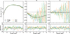 |
Fig. A.1. Spectropolarimetric properties of Cyg X-3 corresponding to the high fluxes with the IXPE count rate above 32 cnt s−1 (see Fig. 3) around orbital phase 0.5. |
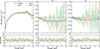 |
Fig. A.2. Same as Fig. A.1, but for the low fluxes with the IXPE count rate below 32 cnt s−1 (around orbital phase 0.0). |
Model parameters for the spectropolarimetric fit for the high and low fluxes.
Then, we performed the same spectropolarimetric analysis checking variation of the orbital-average polarization with time. In particular, we performed the analysis putting together the data in the time bins 2 and 3 and in the time bin 5 (see Fig. 3), corresponding to the highest and lowest PD. The best-fit results are given in Table A.2. The deconvolved spectrum of Stokes parameters I, Q, and U in EFE representation are shown in Figs. A.3 and A.4.
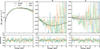 |
Fig. A.3. Same as Fig. A.1, but averaged over the orbital phases during time bins 2 and 3 (see Fig. 3). |
Model parameters for the spectropolarimetric fit for the time bins 2+3 and 5 of Fig. 3.
Appendix B: Radio behaviour at 15 GHz
Cygnus X-3 is monitored at 15 GHz, usually daily, with the Large Array of Arcminute MicroKelvin Imager (AMI; Zwart et al. 2008; Hickish et al. 2018). AMI consists of eight 12.8-m antennas sited at the Mullard Radio Astronomy Observatory near Cambridge, UK. The AMI receivers cover the band from 13 to 18 GHz, and are of a single linear polarisation, Stokes I + Q. Observations are usually made daily, although some are missed due to adverse weather conditions (high winds or heavy rain), or technical issues. Also the number of antennas available varies due to technical issues. Analysis is done using custom software, REDUCE_DC (Perrott et al. 2013). Each observation consists of multiple 10-min scans of Cyg X-3, interleaved with short (∼2-min) observations of a nearby compact source, which were used for phase calibration. The flux density scale is set using nearby observations of 3C 286, which are usually made daily. The day-to-day flux density uncertainty is estimated at ≈5%. Usually short observations, with two 10 min scans are made daily, but sometimes longer observations are made. Figure B.1 shows the AMI observations of Cyg X-3 for several months before and weeks after the IXPE observations. These show that at 15 GHz, Cyg X-3 was in a faint state after a larger outburst in early April. These AMI observations include a longer, ≈4 hour, observation of Cyg X-3 made on 2024 June 3, during the IXPE observations, which is shown in Fig. B.2. The source does not show any pronounced orbital variability in flux density.
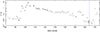 |
Fig. B.1. AMI observations of Cyg X-3 at 15 GHz from early March to mid-June 2024. Each point is the average flux density in a 10 min bin, with an error bar giving the statistical error. The dashed blue line indicates the IXPE observation date. |
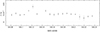 |
Fig. B.2. Same as Fig. B.1, but for the ≈4 h observation (i.e. approximately one orbital period) on 2024 June 3, simultaneous with IXPE. |
Appendix C: Orbital variability
To describe the orbital variability using the rotating vector model, we consider a funnel inclined at angle θ relative to the orbital axis and having azimuthal angle ϕ0 measured in the orbital plane from the line connecting the black hole to the WR star. The orbital axis make angle i to the line of sight. The PA of the scattered radiation can be written as χ = χ0 + χa + π/2, where χa is the position angle on the sky of the orbital angular momentum (measured from north to east) and χ0 is given by the rotating vector model (equation (30) in Poutanen 2020):
 (C.1)
(C.1)
The PD is determined by Eq. (1) where the cosine of the scattering angle varies with the orbital phase as
 (C.2)
(C.2)
The model thus has four parameters: i, θ, χa, and ϕ0. We fitted the ultrasoft-state polarization data with this model obtaining χ2 = 25.7 for 8 dof. The best-fit parameters are  , θ = 3°,
  , and ϕ0 = −120° (i.e. nearly in the direction of motion). This direction is not far from the position of the bow shock (Antokhin et al. 2022) where an excess of the optical depth is expected. We did not try to get the confidence level on the parameters, because the fit is not acceptable.
All Tables
Model parameters for the spectropolarimetric fit for the time bins 2+3 and 5 of Fig. 3.
All Figures
|
Fig. 1. Spectral states of Cyg X-3. Panel a: Radio–X-ray track made by Cyg X-3 as it swings between different spectral states (data from Zdziarski et al. 2016). Panel b: Set of average broadband spectra corresponding to the hard/radio quiescent (blue), intermediate/minor flaring (orange), ultrasoft/radio quenched (black), and soft non-thermal/flaring (magenta) states, as introduced in Szostek et al. (2008). IXPE data are shown with red symbols and the 2σ upper limit at 30 keV (in red) is from Swift/BAT. |
| In the text | |
|
Fig. 2. Average PD and PA as a function of energy. The horizontal dashed lines correspond to the energy-average values. |
| In the text | |
|
Fig. 3. Time variations of the IXPE count rate in the 2−8 keV band and the orbit-average PD and PA. Time is measured from the beginning of the observation at MJD 60463.8124. Boundaries of the time bins (except the beginning and end of the observation) correspond to the orbital phase 0. |
| In the text | |
|
Fig. 4. Orbital phase dependence of the PD and PA from the hard state (blue triangles), the intermediate state (orange open squares), and ultrasoft state (red circles). The green lines show the best-fit rotating vector model (Appendix C) to the ultrasoft-state data. |
| In the text | |
|
Fig. 5. Accretion geometry and parameters of Cyg X-3. Left: Sketch of the geometry associated with the hard, intermediate, and ultrasoft states. The red arrows indicate the direction of the incident and reflected or scattered photons by the optically thick outflow (blue). In the hard state, the only photons reflected at the back surface of the funnel are visible to the observer, while in the intermediate state the reflected and scattered emission is coming from different sides of the funnel (the funnel upper parts become semi-transparent or clumpy). In the soft state, radiation scattered off the matter lying along the funnel axis dominates over the contribution of reflected emission. Right: Polarization of radiation undergoing single scattering above a funnel of half-opening angle α for different observer inclinations i (red lines). The filled red band depicts the conservative PD range 10.8−12.4% of Cyg X-3 in the ultrasoft state, which translates to the inclination of i = 26° −28°; this is very close to the values of |
| In the text | |
|
Fig. A.1. Spectropolarimetric properties of Cyg X-3 corresponding to the high fluxes with the IXPE count rate above 32 cnt s−1 (see Fig. 3) around orbital phase 0.5. |
| In the text | |
|
Fig. A.2. Same as Fig. A.1, but for the low fluxes with the IXPE count rate below 32 cnt s−1 (around orbital phase 0.0). |
| In the text | |
|
Fig. A.3. Same as Fig. A.1, but averaged over the orbital phases during time bins 2 and 3 (see Fig. 3). |
| In the text | |
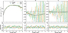 |
Fig. A.4. Same as Fig. A.1, but averaged over the orbital phases during time bin 5 (see Fig. 3). |
| In the text | |
|
Fig. B.1. AMI observations of Cyg X-3 at 15 GHz from early March to mid-June 2024. Each point is the average flux density in a 10 min bin, with an error bar giving the statistical error. The dashed blue line indicates the IXPE observation date. |
| In the text | |
|
Fig. B.2. Same as Fig. B.1, but for the ≈4 h observation (i.e. approximately one orbital period) on 2024 June 3, simultaneous with IXPE. |
| In the text | |
Current usage metrics show cumulative count of Article Views (full-text article views including HTML views, PDF and ePub downloads, according to the available data) and Abstracts Views on Vision4Press platform.
Data correspond to usage on the plateform after 2015. The current usage metrics is available 48-96 hours after online publication and is updated daily on week days.
Initial download of the metrics may take a while.