| Issue |
A&A
Volume 699, July 2025
|
|
|---|---|---|
| Article Number | A157 | |
| Number of page(s) | 15 | |
| Section | The Sun and the Heliosphere | |
| DOI | https://doi.org/10.1051/0004-6361/202554896 | |
| Published online | 04 July 2025 | |
Assessment of sunspot number cross-calibration approaches
1
Max Planck Institute for Solar System Research, Justus-von-Liebig-Weg 3, 37077 Göttingen, Germany
2
Leibniz Institute for Tropospheric Research, Permoserstraße 15, 04318 Leipzig, Germany
3
Institut für Astrophysik und Geophysik, Georg-August-Universität Göttingen, Friedrich-Hund-Platz 1, 37077 Göttingen, Germany
4
Space Physics and Astronomy Research Unit and Sodankylä Geophysical Observatory, University of Oulu, Oulu, 90014, Finland
⋆ Corresponding author: This email address is being protected from spambots. You need JavaScript enabled to view it.
Received:
31
March
2025
Accepted:
30
May
2025
Abstract
Context. Group sunspot number data form the longest record of direct observations of solar activity and variability. However, the observations were conducted by many observers using different telescopes and at diverse locations, which necessitates their proper cross-calibration. Historically, such a cross-calibration was performed with a simple linear scaling. More recently some non-linear approaches have also been developed, as well as modifications of the classical linear scaling. This resulted in a number of new composite sunspot series, which diverge before the 20th century, thus also leading to an uncertainty in the past solar activity and variability.
Aims. Our aim was to understand the causes of divergence between different sunspot series. To this end, we scrutinised the existing cross-calibration methods to identify the sources of their biases and uncertainties.
Methods. We used synthetic data imitating observers with different observing capabilities to test the performance of different cross-calibration approaches, including both simple linear scaling and non-linear non-parametric techniques. Some of these methods require a direct overlap between the records of two observers, while others rely on statistical properties of sunspot groups.
Results. We found that linear approaches generally overestimated and underestimated the maxima of strong and weak activity cycles, respectively, thus introducing a bias in the secular variability. In contrast, for typical characteristics of existing records of observers, non-parametric approaches returned more consistent results and lower errors. Out of these latter, methods relying on statistical properties of the records return worse results.
Conclusions. Our analysis revealed limitations of the various approaches and identified the best approaches. For future recalibrations of sunspot number, we recommend using a direct non-linear calibration when the data coverage is sufficient. However, the errors returned by such daisy-chain methods accumulate when going further back in time, if a multi-step daisy-chain (backbone) calibration is needed. To bridge extensive data gaps, we therefore recommend using a statistical method (e.g. active-day fraction).
Key words: methods: statistical / Sun: activity / sunspots
© The Authors 2025
 Open Access article, published by EDP Sciences, under the terms of the Creative Commons Attribution License (https://creativecommons.org/licenses/by/4.0), which permits unrestricted use, distribution, and reproduction in any medium, provided the original work is properly cited.
This article is published in open access under the Subscribe to Open model.
Open Access funding provided by Max Planck Society.
1. Introduction
Observing sunspots has been referred to as the longest-running experiment in science (Owens 2013). People have observed and recorded information on the appearance and characteristics of spots on the surface of the Sun since the invention of the telescope in 1610 (Vaquero & Vázquez 2009; Arlt & Vaquero 2020). These observations revealed the variable nature of solar activity, manifested in a roughly 11-year periodicity in the number of sunspots (Wolf 1850). The characteristics and conditions of these observations differ significantly because they were conducted by various people using different telescopes at diverse locations, potentially using different grouping conventions or spot-counting practices. This means that they require cross-calibration to a reference level in order to be compiled together in a coherent solar activity index. The first such series was called the Wolf sunspot number, followed by the international sunspot number (ISN; Clette et al. 2023). This quantity was computed as SN=k·(10·G+N), where N is the number of individual spots visible on the solar disc at a given time, G is the number of sunspot groups, and k is a scaling factor to bring the records of an observer to the level of a chosen reference observer. This activity index is not based solely on the counts of individual sunspots because of the increased uncertainty in recovering that quantity for earlier observations, while the number of groups is more robustly recovered. The lack of information on individual sunspots limited the extent of the daily series back to 1818, while annual data could be compiled back to 1750 and, with large uncertainties, to 1700.
With the aim of incorporating the earliest available sunspot data and lift uncertainties in the counts of individual sunspots, Hoyt & Schatten (1998) proposed a different sunspot activity index, based solely on the number of sunspot groups (hereafter GSN). For many years, these two indices were the main direct solar activity records covering extended periods, while records of plage areas (since 1892; e.g. Chatzistergos et al. 2020, 2022b), Hα filament areas (since 1909; e.g. Chatzistergos et al. 2023a), or F10.7 emission (since 1947; e.g. Tapping 2013) cover significantly shorter periods. In this respect, sunspot series have been widely used in a number of applications, particularly for studying solar magnetism, extending chromospheric indices (e.g. Yeo et al. 2020; Clette 2021; Chatzistergos et al. 2022a), and reconstructing solar irradiance variations (Foukal & Lean 1990; Solanki & Fligge 1998; Krivova et al. 2007, 2010; Dasi-Espuig et al. 2016; Wu et al. 2018; Wang & Lean 2021; Chatzistergos 2024), with important implications for studies of the solar influence on Earth's climate (Haigh 2007; Gray et al. 2010; Solanki et al. 2013; Krivova 2018; Chatzistergos 2023; Chatzistergos et al. 2023b). This highlights the importance of having information on past solar activity that is as accurate as possible, and thus in particular of sunspot number and group sunspot number series.
More recently, sunspot records have been scrutinised in more detail. It was realised that there were many inconsistencies in the raw sunspot data (see e.g. Vaquero et al. 2016; Clette et al. 2023) as well as issues with the cross-calibration approaches, especially on the applicability of a linear scaling between the records of different observers (Lockwood et al. 2016b; Usoskin et al. 2016a). Sunspot and group number counts reported by individual observers can be affected by various factors, including telescope aperture, atmospheric seeing conditions, and the type of detector used (e.g. the human eye, photographic plates, or modern electronic sensors). These factors collectively determine the observer's acuity, which defines the smallest sunspot group they are able to discern. Several studies (e.g. Usoskin et al. 2016a; Chatzistergos et al. 2017; Karachik et al. 2019) have shown that the number of individual spots and groups changes non-linearly with observational acuity or telescope aperture. The above led to the development of a number of alternative GSN series by using different cross-calibration techniques (Svalgaard & Schatten 2016; Cliver & Ling 2016; Usoskin et al. 2016b, 2021; Chatzistergos et al. 2017; Willamo et al. 2017) as well as versions 2–2.3 of the ISN (Bhattacharya et al. 2023, 2024). It should be noted that while the GSN series can be re-built from scratch using the raw sunspot group data (Vaquero et al. 2016), the ISN has not been fully revisited yet because of the lack of raw data, which are presently in the process of restoration (Clette et al. 2023). Some of these alternative series are shown in Fig. 1. Furthermore, corrections of existing sunspot records (e.g. Hayakawa et al. 2021; Carrasco et al. 2021a, 2024) and the recovery of new sunspot records (e.g. Carrasco et al. 2021b; Hayakawa et al. 2022, 2024; Ermolli et al. 2023) is an ongoing process (e.g. Vaquero et al. 2016; Clette et al. 2023) that has also improved sunspot number compilations over the early telescopic periods (e.g. Vaquero et al. 2015; Carrasco et al. 2022, 2024). However, despite all the advances, there are still significant disagreements between various individual sunspot number composites. These reconstructions generally agree over the 20th century, but strongly diverge before about 1880. The existing sunspot series can be roughly divided into three groups according to their implied mean activity level over the 18th and 19th centuries: high (Svalgaard & Schatten 2016; Cliver & Ling 2016); low (Hoyt & Schatten 1998); and moderate (Chatzistergos et al. 2017; Usoskin et al. 2021).
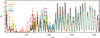 |
Fig. 1. Group sunspot number series by Hoyt & Schatten (1998, HoSc98, yellow), Svalgaard & Schatten (2016, SvSc16, dashed red), Chatzistergos et al. (2017, CEA17, dashed green), Usoskin et al. (2021, UEA21, cyan), and Velasco Herrera et al. (2024, VHS24, black). Shown are annual mean values. |
One possible contributor to this divergence is the difference in the cross-calibration technique used in the various studies. We tested the effect of the cross-calibration techniques on the resulting sunspot number composite by applying them to synthetic records simulating various observers with known characteristics. Here we discuss only GSN since the digitisation of the raw counts of individual sunspots needed to recalibrate ISN is still ongoing, but our results are applicable to ISN as well and will be useful for the preparation of the upcoming recalibration of ISN leading to its version 3 (Clette et al. 2023).
The paper is structured as follows. Section 2 provides an overview of the synthetic data we used as well as the cross-calibration techniques that we tested. Section 3 presents our results. We draw our conclusions in Sect. 4.
2. Data and methods
2.1. Data
For our analysis we used a large set of synthetic sunspot data generated previously (Chatzistergos et al. 2017; Chatzistergos 2017). These synthetic data are based on the observations of the Royal Greenwich Observatory (RGO)1 between 1874 and 1976 (Willis et al. 2013). However, due to some concerns about the stability of early RGO data expressed in the literature (Clette et al. 2014; Cliver & Ling 2016; Lockwood et al. 2016b), only data after 1900 were considered. The RGO database includes information about the area and location of individual sunspot groups for each day. Based on this, Chatzistergos et al. (2017), Chatzistergos (2017) created records of various artificial observers by imposing different acuity thresholds, A, defined as the lowest area of a sunspot group that the observer can discern. This way we emulated imperfect observers, while the original RGO data can be considered as perfect. Thus, evaluating different cross-calibration methods on such synthetic data and comparing the results to the original RGO data allows us to estimate the accuracy of the methods in certain controlled situations (e.g. different known acuities or overlaps). In the following, we refer to such synthetic observers as RGOXXX where XXX is the value of the acuity threshold, A, in units of millionths of the solar disc (msd). We used 121 different synthetic observers produced with acuity thresholds that ranged from 0 to 300 msd. These thresholds include all the integer values between 0 and 100 msd and every tenth integer between 100 and 300 msd.
We note that actual observational reports may also vary due to differences in grouping conventions, spot-counting practices, the possible use of weighting schemes, or changes in observer acuity over time (e.g. due to varying weather conditions or declining eyesight). These factors are expected to introduce additional uncertainty in the calibration process across all methods, which we do not consider here.
2.2. Cross-calibration methods
Here we present the five cross-calibration approaches that have been used to produce group sunspot number composites, namely those by Hoyt & Schatten (1998, HoSc98, hereafter), Svalgaard & Schatten (2016, SvSc16, hereafter), Chatzistergos et al. (2017, CEA17, hereafter), Usoskin et al. (2021, UEA21, hereafter), and Velasco Herrera et al. (2024, VHS24 hereafter). We describe each of these methods below. One more cross-calibration approach, shown by Clette et al. (2023, there referred to as DuKo22), utilises the tied-ranking of observer counts and has been employed to produce a group number series. However, we do not consider this method here for two reasons: firstly, it has not yet been fully published and described; secondly, its applicability on historical records is not straightforward as it requires reference-observer data for all days when the secondary observer reported counts, necessitating extrapolation, and thus introducing uncertainty.
2.2.1. HoSc98
Hoyt & Schatten (1998) scaled daily records of sunspot groups by different observers linearly. The scaling parameter for a given observer was determined as
 (1)
(1)
where G* is the group count by the primary observer and G the group count by the observer in question, while the summation is over all days on which both observers counted at least one sunspot group. In addition, Hoyt & Schatten (1998) set a threshold on kHoSc98 such that the counts of a given observer were only used if 0.6<kHoSc98<1.4. For example, the synthetic observer RGO010 (i.e. with an acuity threshold A = 10 msd) would receive a calibration factor of kHoSc98 = 1.12 to be cross-calibrated to the original RGO data (see light blue line in Fig. 2).
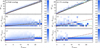 |
Fig. 2. Calibration matrix for the method by Chatzistergos et al. (2017) between RGO and a synthetic observer with acuity threshold A = 10 msd (that is RGO010). The matrices show probability mass functions, which are colour-coded (see colour bars to the right of each panel). The top panels show the matrices with the actual records, while the middle and bottom panels show the matrices for the difference of the counts of the observers. In the bottom panel, the columns of the matrix that had insufficient statistics were filled with a Monte Carlo bootstrap simulation. The left-hand column is for the full period of RGO observations, while in the right-hand column only 1% of the randomly selected days were considered (see Sect. 3.3). The red circles with error bars give the mean values within each column and the 1σ intervals. The green curve shows the fit represented by Eq. (3), while the scalings for HoSc98, SvSc16, and VHS24 are shown in dashed cyan, red, and black, respectively. We recall that SvSc16 was determined for annual values. The solid black line in the top panels denotes a slope of unity. |
2.2.2. SvSc16
Svalgaard & Schatten (2016) also applied a linear scaling between the group counts. However, in their approach, the scaling factor is determined with a linear regression of annual mean values computed for both observers, irrespective of the exact overlap of the days of their observations. For data from each observer, they first computed monthly means and then from those the annual means, considering all months that had at least one observation by this observer. The applied linear regression was forced through the origin, thus assuming that 0 in the counts of one observer is always 0 for the other observer's counts too (cf. Usoskin et al. 2016a; Lockwood et al. 2016a). The scaling factor in this method is thus defined as
 (2)
(2)
where Y* and Y are the yearly average group counts of the primary observer and the secondary observer, respectively. Although Svalgaard & Schatten (2016) mention that they checked the goodness of their fits, they do not explicitly specify under which conditions (if at all) the data from a given observer would not be used for the cross-calibrated record. It is also worth noting that annual means were derived for the primary and secondary observers on their respective observational days, not only on their common days. Thus, annual means underlying the comparison might eventually be derived from observations on different days, which can lead to biases. For the synthetic observer RGO010, for example, we obtained kSvSc16 = 1.12 needed to cross-calibrate this record to the original RGO data (see red line in Fig. 2).
2.2.3. CEA17
The third cross-calibration approach is the one by Chatzistergos et al. (2017). It was first introduced by Usoskin et al. (2016a, b), and Bhattacharya et al. (2024) used its variation. This approach uses conversion matrices of probability mass functions (PMFs) of group counts by different observers. For this, a normalised histogram of group counts reported by the reference observer is computed for all days for which the secondary observer reported a given group count. The normalised histograms for different group counts of the secondary observer are stitched together into a calibration matrix so that each column represents a PMF. The resulting calibration matrices are then used to determine the most probable value for the reference observer's count given a specific count of the secondary observer. An example of such a PMF for the synthetic observer RGO010 is shown in Fig. 2a).
Some of the columns of the matrices produced in this way remain empty or do not have sufficient statistics to accurately describe the relation between the two observers’ counts. A bootstrap Monte Carlo simulation was performed to fill these columns. We randomly selected half of the overlapping days to produce a separate matrix and fitted the difference between the mean of the PMF of each column,  , and the count of the secondary observer, G, with the equation in the form
 (3)
(3)
where R0, B, and a were free parameters of the fitting. This process was repeated 1000 times. The resulting 1000 fits (Eq. (3)) were then used to create a probability distribution function matrix from them. This matrix was then employed to replace the columns in the initial PMF with insufficient statistics. An example calibration matrix for the synthetic observer RGO010 is shown in Fig. 2. In particular, the top panels show the initial matrix, while the middle panels show the difference between the records of the two observers to help highlight the non-linearity of the relationship. It is evident that the last five columns do not have sufficient statistics; they were thus replaced by the results of the Monte Carlo simulation, as shown in the bottom panel for the difference matrix. The calibration was then performed by replacing each single group count of the secondary observer with the PMF of the corresponding group count column. This way, the calibration returns a PMF series, which also includes information about the uncertainty of the records and not just a single value as in other methods.
To ensure sufficient and proper statistics for accurate cross-calibration, CEA17 further considered a number of additional criteria. These, in particular, include a lower limit of 20 overlapping days between the two observers and an overlap of more than four years for long-running observers (to avoid spurious long-term trends). In addition, the matrix must have sufficient statistics for at least three columns and one-quarter of the range of counts by the secondary observer, or the difference between the two records in question for counts below five groups should be lower than two groups. An additional constraint was imposed by considering the metrics of the fit (Eq. (3)): if the fit returned a χ2 per degree of freedom greater than 6 the observer was not considered.
2.2.4. UEA21
The fourth method is the one by Usoskin et al. (2016b, 2021), Willamo et al. (2017, 2018). The great benefit of this method over those described above is that it does not require a direct overlap between the observers. The calibration is done with PMF matrices as in the CEA17 method. However, instead of comparing the two observers directly over their overlapping days, UEA21 makes use of the statistics of active days (days with at least one sunspot group reported). This means that the PMF matrices are pre-constructed from the synthetic RGO data for different acuities, while the acuity threshold of each observer is determined from the statistics of active days. For a given observer, this is achieved by computing the cumulative distribution of active days within each month and comparing it to reference distributions constructed from the synthetic RGO data for different acuities and different temporal coverages. The reference curve that minimises the sum of squared residuals to that of the observer's is taken as the acuity threshold of the observer, and thus determines which PMF matrix should be used for the calibration.
2.2.5. VHS24
The last method is the one by Velasco Herrera et al. (2024). This is another linear scaling method where the scaling parameter is defined as
 (4)
(4)
where σG and  are the standard deviations of the counts of the secondary and the reference observer, respectively. In contrast to the HoSc98 and SvSc16 methods, VHS24 did not force this relation to the origin, but considered an additive parameter b so that
 (5)
(5)
where 〈G〉 and 〈G*〉 are the mean value of the entire records of the secondary and reference observers, respectively.
This method was also applied on data without direct overlap by considering the records from Kislovodsk to be the reference. Since we want to evaluate the performance of the methodology, here we consider the entire record of RGO as the reference (i.e. since 1900). For the synthetic observer RGO010, for example, we obtained kVHS24 = 1.09 and b = 0.16 needed to cross-calibrate this record to the original RGO data (see black line in Fig. 2).
This methodology is marked by serious limitations. In particular, a big limitation of this method is that the standard deviation of values, which is used to determine the scaling parameter, is variable over the solar cycle, being typically lower during activity minima than during maxima. Considering that the scaling applied by VHS24 has no way of establishing that it compares records from similar activity levels, it is thus expected that it will lead to random artefacts. The authors also did not present any evaluation of whether this approach can be applied to data without a direct overlap and if it returns consistent results. However, we include it here for the sake of completeness.
3. Comparison of the methods
Figure 2 provides a first comparison between the various methods for calibration of the synthetic observer RGO010 to the original RGO data. We show the PMF matrix used for the calibration for the CEA17 and UEA21 methods, as well as the relations for the other three methods (all represented by straight lines). The resulting cross-calibration relationships differ significantly, in particular they exhibit different behaviours for low and high group counts, in this case below and above about 6–8 groups. The fit used for the CEA17 method follows rather well the mean values within each column of the PMF matrix. Relative to that, the scaling applied with all three linear methods leads to greater overestimations of high group counts, which is about 1 group when RGO010 reported 24 groups. The opposite behaviour is seen for a low number of groups, where the method by CEA17 leads to slightly higher values than those of the linear methods. Similar comparisons with records of actual observers can be seen in Usoskin et al. (2016a), Chatzistergos et al. (2017), Chatzistergos (2017). The above comparison suggests that the CEA17 and UEA21 non-linear methods are more accurate in performing the cross-calibration for daily values since they are able to capture the non-linearity of the relationship, while the methods by HoSc98, SvSc16, and VHS24 lead to an overestimation of high group counts as well as a slight underestimation of low group counts. We note that the acuity threshold of 10 msd, discussed here for illustration, corresponds to a relatively good observer, while the discrepancy may be stronger for observers with poorer instrumentations available during earlier centuries. In the following, we discuss in detail this comparison by also considering the effect of the acuity of the observer and the activity levels on the outcome.
3.1. Performance of methods for varying acuities
We applied the CEA17, HoSc98, UEA21, VHS24, and SvSc16 methodologies that were introduced in Sect. 2 to cross-calibrate all synthetic observers. Given that the SvSc16 series contains only annual values, we first computed the annual means for all methods from the calibrated records of synthetic observers to ensure direct comparability. We then compared them with the annual values of the original RGO data.
Figure 3 compares the standard metrics describing the quality of the calibrations to the original RGO for reconstructions with each of the five methods for given acuities. In particular, we show the RMS, mean, relative unsigned, and maximum absolute differences for all cross-calibration techniques. In terms of these metrics, SvSc16, VHS24, and HoSc98 return very similar results, while CEA17 and UEA21 behave differently. We note here that for these metrics, CEA17 and UEA21 are by design identical as they used the same calibration matrices. That is because this is an idealised case for UEA21 where the same data that were used to produce the reference calibration curves were also used as the secondary observer's data, and thus the method has no uncertainty in determining their acuity thresholds. In terms of RMS differences, CEA17 performs slightly better than other methods for acuity thresholds lower than about 30 msd, but worse for greater acuities. In contrast, the maximum absolute difference is higher for CEA17 for acuity thresholds below 20 msd and lower afterwards. The mean differences show the highest spread among the methods, being consistently very close to zero for CEA17, UEA21, and VHS24, while constantly decreasing with increasing acuity for HoSc98 and SvSc16, which implies that the overall mean value is consistently underestimated by these methods. This suggests that the methods by HoSc98 and SvSc16 introduce a systematic bias that increases with acuity, while the other methods return rather symmetric errors that almost completely balance out over solar cycle timescales.
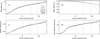 |
Fig. 3. Differences between reconstructions using the methods CEA17 (green), UEA21 (light blue), SvSc16 (purple), VHS24 (black), and HoSc98 (red), and the original RGO group number series for different acuities. The reconstructions were done for the entire period of RGO record. Shown are the RMS (a), mean (b), relative unsigned (c), and maximum absolute (d) differences. We note that by design, CEA17 and UEA21 are identical in these metrics in this case. The vertical dashed lines indicate the acuity threshold beyond which the respective method excludes the observer based on its quality criteria (see Sect. 2.2). |
Figure 4 shows how well the different methods cross-calibrate the various synthetic observers in comparison to the original RGO counts as a function of time. In particular, Figures 4b-f) show the differences between the cross-calibrated counts of synthetic observers and the original RGO counts for nine acuity thresholds (A = 1, 3, 5, 10, 20, 30, 50, 100, and 300 msd). The differences are given as  , where
  is the calibrated group number of synthetic observer with acuity A, and G0 is the original RGO data, which is the synthetic observer with acuity A = 0 msd. For comparison purposes, Figure 4a) shows the difference of the raw counts of the synthetic observers to the original values from RGO. Figure 4 highlights further the differences in the results provided by the various cross-calibration techniques. In particular, both HoSc98 and SvSc16 overestimate or underestimate activity for the strongest or weakest cycles, respectively. The higher the acuity threshold, the stronger this effect is. This conforms to the expectations for such approaches, as discussed at the beginning of Sect. 3. In contrast, the methods by CEA17, UEA21, and VHS24 show a more coherent behaviour: with increasing acuity they habitually underestimate activity maxima and overestimate activity minima, albeit typically to a lesser degree than HoSc98 and SvSc16. Thus, the key difference between the methods can be summarised as follows. CEA17, UEA21, and VHS24 typically overestimate (underestimate) activity minima (maxima), independently of the mean activity level. At the same time, the other methods introduce an error that depends on the activity level, such that the amplitudes of weak and strong cycles are skewed in opposite directions, leading to unwanted systematic effects. The HoSc98 and SvSc16 approaches return yearly averages that differ less from the yearly averages of the primary observer during periods of low solar activity compared to the CEA17 approach. The elevated values at activity minima resulting with the CEA17 method are expressions of the uncertainty of the cross-calibration, which increases with increasing acuity threshold. This uncertainty is ignored by the HoSc98 and SvSc16 methods, which force the relation through the origin. Thus, for these methods when the secondary observer reported 0 groups it will always be 0, also in the calibrated data.
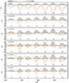 |
Fig. 4. Difference between group counts of synthetic data of different acuity to the original RGO data ( |

Figure 4 and the above discussions make it clear that the uncertainties of the cross-calibration increase with the increasing acuity of the observers independently of the method. This highlights the importance of employing, whenever possible, records of comparatively similar quality. In Fig. 4 we also mark the cases for which the criteria imposed by the respective method would exclude an observer. In particular, CEA17 would exclude observers with A≥87 msd, while the limit for HoSc98 is A≥31 msd. VHS24 and SvSc16 did not mention any quality criteria. These limits, marked in Fig. 4, indicate that for all acuities considered by HoSc98, its performance is worse than that of CEA17. We note that many of the real observers back to 1749 have an estimated acuity threshold below 60 msd (Usoskin et al. 2016b). We also emphasise here that for the methods requiring a direct overlap between two observers, the acuity is a relative measure between these two specific observers, and thus it is expected to be relatively low and rather unlikely to reach very high values. On the contrary, for the two methods that do not require a direct overlap between the observers, acuities can become rather high. For these methods, the acuity difference is defined relative to a 20th-century observer, and thus almost systematically increases (i.e. worsens) going back in time.
Finally, we note that the results presented in this section are for the idealised situation when there is a 100% overlap between the records of the secondary and reference observers, which is rather unlikely to occur with actual observers. Thus, the errors of the various methods presented here can be considered a low limit. In the next sections we discuss how the various cross-calibration approaches handle incomplete overlaps between the two observers.
3.2. Performance of methods for activity levels outside of those used for the reconstruction
In this section we analyse the impact of the training interval on the outcome of the cross-calibration with various methods. In particular, we removed some SCs when constructing the calibration relationships and evaluated how well the different techniques were able to calibrate the data.
Figures 5–7 show the differences between the calibrated series constructed with each method by removing some individual SCs from the fitting process and those obtained using all data available for the calibration. The values shown in Figures 5–7 are effectively the deviations from those shown in Fig. 4 and they thus highlight the effect of the removal of specific data on the calibration process. These are expressed as  , where
  is the calibrated group number of the synthetic observer with acuity A using all data, and
  is the same, but when excluding solar cycle SC from the cross-calibration.
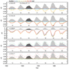 |
Fig. 5. Sensitivity of the cross-calibration methods (as denoted in each panel) to activity levels during periods used to build the conversion relationships. Shown are the differences between the calibrated group counts for the synthetic data (cycle 16 was excluded from the calibration) and for the data where all cycles were considered for the calibration ( |

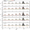 |
Fig. 6. Same as Fig. 5, but this time SC 19, the strongest cycle over the considered period, is excluded from the calibration. |
Figures 5 and 6 show the results by removing a single SC. In particular, we removed SC 16, which is one of the weakest cycles within the RGO data and SC 19, the strongest cycle on the record. We considered SC 16 and not SC 14 so as to be on the conservative side, due to the potential issues with early RGO data extending up to 1915 (Clette et al. 2014; Cliver & Ling 2016; Lockwood et al. 2016b). We find that removing a weak SC like SC 16 has a rather weak effect on the calibration with all methods. UEA21 is the method that is the least sensitive to removing a weak cycle such as SC 16. The acuity of the observers was precisely determined from the statistics of active days in all but three cases shown here (with acuities of 1, 5, and 100 msd). This means that the errors introduced by this method when removing SC 16 are typically as low as when considering the full dataset. Small discrepancies sometimes arise from inaccuracies in estimating observer acuity (e.g. for acuities of 1, 5, and 100 msd shown in Fig. 5), which affect the selection of the appropriate calibration matrix. Among the other methods, the smallest effect is found for CEA17, which for example exhibits changes that are lower than 0.03 for the synthetic observer RGO050, while for the same observer a difference of -0.06 and -0.08 is reached for HoSc98 and SvSc16, respectively. The errors with VHS24 exceed −0.3 and are in general about four times higher than for the other methods. While all other methods return minute errors for low acuities, this is not the case for VHS24. The results for VHS24 are very similar for all acuity thresholds tested, meaning that the effect of the missing statistics for one cycle has a significantly greater effect in this method than the acuity of the synthetic observers. For CEA17, missing the statistics of SC 16 leads to a slight increase in the values during activity maxima, while the effect on minima is smaller. For the HoSc98, SvSc16, and VHS24 methods, in contrast, the values during all activity maxima rise. The only exception is the synthetic observer RGO300 when using HoSc98, although in this case the derived scaling parameter would render this observer to be excluded in any case.
Removing a strong cycle like SC 19 has a stronger impact on the calibration. The methods by VHS24 and SvSc16 return the highest errors. They overestimate all values during activity maxima, with differences reaching up to about 1.5 and 0.3, respectively, for the synthetic observer RGO050. HoSc98 also overestimates the values during activity maxima, although only by about half that of the SvSc16 method. The method by CEA17 tends to underestimate the values during maxima. However, we find for synthetic observers RGO001 to RGO010 that the effect is minute, while it increases to about −0.1 for synthetic observers RGO020 and RGO030. UEA21 systematically overestimates the acuity of the observer, thus in the end also amplifies the group numbers. This error decreases for higher acuities, and becomes 0 for 300 msd. This is an artefact, however, since 300 msd was the highest acuity considered for the synthetic observers used to produce the reference curves. This introduces a cap in the determined acuities with the UEA21 method.
Finally, Figure 7 shows the results when all SCs after SC 15 were removed. We also tested the case when all SCs before SC 19 were removed (not shown here). For the cases of removing all SCs before SC 19 and all after SC 15 the effect was qualitatively the same as removing SC 16 and SC 19, respectively. That is, HoSc98, SvSc16, UEA21, and VHS24 systematically underestimated (overestimated) the group counts by removing weak (strong) cycles from the calibration process. CEA17 exhibits the opposite behaviour for most acuities; however, CEA17 typically also returns the lowest errors. Also in this case, VHS24 and SvSc16 perform worse than the other methods. We note that for VHS24 the errors become quite significant, exceeding two and five groups when removing all cycles after SC 16 and before SC 19, respectively, while the errors are quite consistent for all the acuities tested here. Thus, as previously reported, the main error with VHS24 is methodological and is due to comparing the statistics of group records over different periods that are actually not comparable. The errors for UEA21 also become significant, reaching up to four groups when all SCs after SC 15 are excluded. However, when all cycles before SC 19 are excluded, the errors are lower, up to about two groups, and are mostly below one group. This might hint at issues with the early RGO data, that there are big differences in the active day fraction statistics over different periods of RGO data, or that the process used to estimate the acuity of observers in the UEA21 method needs improvement. We note that qualitatively our results for UEA21 here are consistent with those by Willamo et al. (2018).
Figure 8 compares the RMS differences of the records cross-calibrated with the SvSc16, HoSc98, UEA21, and VHS24 methods to that using CEA17. The RMS difference returned by each method minus the RMS difference of CEA17 are shown both for the annual means (left column) and the daily values (when available; right column). Thus, positive (negative) values mean that CEA17 performs better (worse) than the other respective method. We find that in general CEA17 performs better than all methods for acuity thresholds below about 30 msd. When excluding some SCs the results are similar. The biggest difference is seen when removing SCs 16–20, when the better performance of CEA17 is most pronounced. However, when removing SCs 14–18, CEA17 offers only a marginal improvement compared to HoSc98 and SvSc16, while the HoSc98 performs better for acuities above 12 msd. For daily values, the results for UEA21 and VHS24 are qualitatively the same as for the annual means, although the differences are slightly lower. However, comparing CEA17 to HoSc98 for daily values we find a consistently better performance for CEA17 with increasing acuity.
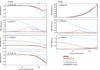 |
Fig. 8. Comparison of RMS differences returned by the various methods with that of CEA17 by considering different calibration periods. The curves are shown as the RMS difference of each method (as denoted in each panel) minus the RMS difference of CEA17 (positive and negative values mean CEA17 performs better and worse than the respective method, respectively). |
Figure 9 illustrates the mean difference between the cross-calibrated series and the original RGO series as a function of acuity. For HoSc98, the mean difference decreases with increasing acuity. However, when SCs 16–20 are excluded, HoSc98 leads to a slight overestimation of most moderate acuities before also turning to an underestimation. For SvSc16, the mean differences also decrease with increasing acuity, although when excluding SCs 16–20 they instead steadily increase. CEA17 provides overall more stable results; however, also with this method the mean difference is affected for acuities exceeding approximately 20 msd. In contrast, VHS24 shows substantial offsets across different periods used for cross-calibration. This discrepancy arises from their flawed assumption that the standard deviation of sunspot counts remains unchanged over different activity levels.
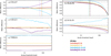 |
Fig. 9. Comparison of mean differences of calibrated to original RGO data for the various methods by considering different calibration periods. The vertical dashed lines indicate the acuity threshold beyond which the respective method excludes the observer based on its quality criteria (see Sect. 2.2). |
In summary, the SvSc16, VHS24, and UEA21 cross-calibration approaches are very sensitive to the periods covered by the data used for the calibration that might lead to significant uncertainties. The uncertainties are lower for HoSc98 and CEA17. This means that for daily values CEA17 performs better for all acuities tested here, while for the annual means it returns better and more consistent results for acuity thresholds lower than about 30 msd.
3.3. Performance of methods for reduced overlaps
In this section we compare the performance of the cross-calibration methods by reducing the overlap between the observers. We did this by randomly removing days from the reference observer so that the overlap with the secondary observer had the following values: 50%, 20%, 10%, 7%, 5%, 4%, 3%, 2%, and 1%. For each case we performed the calibration 100 times by randomly selecting different days achieving the desired overlaps. The same subsamples of days were used for all cross-calibration methods.
Figure 2 shows examples of the calibration relations for the different methods for RGO010, considering the entire record (left column) and one realisation with only 1% of the data (right column). All three methods applying linear scaling (HoSc98, SvSc16, and VHS24) give a higher value for the scaling factor for the 1% coverage compared to the full series (kHoSc98 = 1.13, kSvSc16 = 1.19, and kVHS24 = 1.17 and b = 0.25). For CEA17, the mean values in each PMF are only minutely affected, although the reduced statistics influence the width of individual PMFs, and thus the uncertainty of the reconstruction. Figure 10 shows the difference of the group numbers of RGO010 calibrated with the various methods to the original RGO counts. These are expressed as  , where
  is the calibrated group number of the synthetic observer with acuity A using all the data, and
  is the same but with a reduced coverage RC.
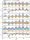 |
Fig. 10. Comparison between RGO010 and RGO000 group counts, represented as the differences between the raw data ( |


The method by CEA17 returns the smallest differences and most consistent results compared to the other methods, which, in addition to returning higher errors, also introduce a bias by increasingly overestimating the maxima with decreasing coverage. UEA21 returns very high errors when the coverage is very low, although reaches similar values to CEA17 with increasing coverage.
The calibrations with the SvSc16 and VHS24 methods are significantly affected by data gaps. On average, reduced coverage results in an overestimated activity. However, depending on the selected days, random errors can lead to measurable over- or underestimation of group counts.
Figure 11 presents a comparison of the RMS differences between the calibrated and original records as a function of observer overlap. For acuity thresholds below 30 msd, CEA17 performs better than the other methods for annual values if the overlap is at least 3% of the length of the reference observer (Figure 11). The results are qualitatively similar when comparing the daily values, although for RGO001 HoSc98 performs better for overlaps lower than 20%, while CEA17 progressively performs better than HoSc98 and the other methods for all overlaps with increasing acuity. The errors with SvSc16, VHS24, and UEA21 are typically more affected with a reduction in observer overlaps than CEA17 or HoSc98. However, UEA21 becomes closer to CEA17 with increasing coverage.
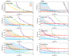 |
Fig. 11. Comparison between the performance of the various cross-calibration methods on synthetic observers as a function of overlap to the original RGO data. Shown are the results for synthetic observers with acuity thresholds of 1 (a, e), 5 (b, f), 10 (c, g), and 30 (d, h) msd. The shaded surfaces mark the range due to the 100 realisations for each case of overlap, but to ease visibility are shown only for CEA17 and HoSc98. The RMS differences are computed for the annual values (left column) and the daily values (right column). The horizontal black line marks the differences if the raw data are used uncalibrated (shown only at the top panels). |
4. Summary and conclusions
The number of sunspots is the longest and most used direct metric of solar activity. Having an accurate sunspot number series is crucial for studies of past solar magnetism, reconstructions of irradiance variations (Chatzistergos et al. 2023b), and thus also for understanding the Sun's influence on Earth's climate (Solanki & Unruh 2013; IPCC 2021). However, construction of a consistent and accurate record is a complicated task. This is, to a large extent, because the available data come from many observers with significantly different observing capabilities, which results in quite diverse levels of quality of the data. The first such series, introduced by Rudolf Wolf, is now called the international sunspot number series; later on, additional series of sunspot group counts were also introduced. Historically, the cross-calibration of the available records had long been performed with a simple linear scaling introduced by Wolf in the mid-19th century. Various issues with this approach have been reported in the literature (see e.g. Clette et al. 2023), which led to the construction of a number of alternative sunspot number series using different methodologies. The existing reconstructions of group sunspot numbers diverge before the 20th century. The existing cross-calibration methods can be divided into those that require a direct overlap between observers (CEA17, HoSc98, and SvSc16) and those that perform the calibration based on statistical properties of the series (UEA21 and VHS24). Alternatively, they can also be divided into those applying a linear scaling of the data, which are in fact most of the methods (e.g. HoSc98, SvSc16, and VHS24) or non-linear and non-parametric methods (CEA17 and UEA21).
Here we performed a sensitivity study of the commonly used cross-calibration techniques. In particular, we used synthetic data generated with a broad range of acuities to simulate historical observers. This allowed us to quantify calibration errors and evaluate the methods in cases of suboptimal observer overlap. By specifically excluding strong or weak cycles from the cross-calibration, we assessed the performance of the methods under these various conditions.
The accuracy of cross-calibration methods varied with observer acuity, with errors increasing for higher acuities for all the methods used. This highlights the importance of employing records of similar quality whenever possible. We found that the non-linear calibration methods (CEA17 and UEA21) performed more consistently than the linear methods for observers with different acuities and different overlapping periods. The linear calibration methods (HoSc98, SvSc16, and VHS24) systematically amplify strong cycles and underestimate weak cycles.
The exclusion of weak or strong solar cycles impacted the calibration differently across methods. Removing a weak cycle like SC 16 had a minimal effect in all methods (except VHS24), with CEA17 and UEA21 being the least affected. Removing a strong cycle like SC 19 led to larger errors, particularly for VHS24 and SvSc16, which tend to overestimate values during activity maxima. Generally, removing a weak cycle from the calibration period led to underestimated activity maxima for the linear methods (HoSc98, SvSc16, and VHS24), while removing a strong cycle resulted in an overestimation. The non-parametric methods (UEA21 and CEA17) exhibited the opposite trend.
Data gaps significantly impact SvSc16 and VHS24, on average leading to exaggerated activity for decreasing coverage. For reduced coverage, even for low-acuity observers, HoSc98, SvSc16, and VHS24 consistently overestimate activity maxima, whereas CEA17 performs better. For annual values and acuity thresholds below 30 msd, CEA17 outperforms HoSc98 when the observer overlap is at least 3% of the reference period. For daily values, HoSc98 performs slightly better for overlaps below 20%, but CEA17 progressively improves with increasing acuity and coverage. Overall, CEA17 emerges as the most reliable cross-calibration method, maintaining accuracy across different conditions and minimising biases that affect other methods, particularly under limited data availability.
It is noteworthy that all methods returned pronounced differences to RGO over SC 15. We see this even for the case of RGO001. This might be an indication that there are indeed residual consistency issues with the RGO data over this cycle, as has been previously argued by Sarychev & Roshchina (2009), Clette et al. (2014), Cliver & Ling (2016), Lockwood et al. (2016b).
It is important to note that methods requiring a direct overlap between the records of observers (CEA17, HoSc98, and SvSc16) are expected to return errors that accumulate with an increasing number of connections when going further back in time. The effect of the daisy-chaining process was not evaluated in this study, but it would be important to address it in forthcoming studies. Complications for this are that each of the above-mentioned studies used daisy-chaining in a different way, while HoSc98 did not even provide sufficient documentation to replicate their process. The UEA21 and VHS24 methods do not have this issue. However, we note that these methods carry the implicit assumption that the statistical property they use remains stable in time. UEA21 considers the statistics of active days, while VHS24 uses the standard deviation of group counts. Since the standard deviation of the group counts changes dramatically with the activity level and period covered, the latter is a methodological drawback of the VHS24 method.
Overall, it is recommended to use a direct calibration based on the observer's acuity threshold when the data coverage is sufficient (e.g. CEA17). A statistical method (e.g. UEA21 based on the active-day fraction) should be used to bridge extensive data gaps.
Acknowledgments
This work was supported by the European Union's Horizon 2020 research and Innovation program under grant agreement No 824135 (SOLARNET). This project has received funding from the European Research Council (ERC) under the European Union's Horizon 2020 research and innovation programme (grant agreement No. 101097844 – project WINSUN). This study has made use of Smithsonian Astrophysical Observatory (SAO)/NASA's Astrophysics Data System (ADS; https://ui.adsabs.harvard.edu/) Bibliographic Services.
Available at https://solarscience.msfc.nasa.gov/greenwch.shtml
References
- Arlt, R., & Vaquero, J. M. 2020, Liv. Rev. Sol. Phys., 17, 1 [NASA ADS] [CrossRef] [Google Scholar]
- Bhattacharya, S., Lefèvre, L., Hayakawa, H., Jansen, M., & Clette, F. 2023, Sol. Phys., 298, 12 [Google Scholar]
- Bhattacharya, S., Lefèvre, L., Chatzistergos, T., Hayakawa, H., & Jansen, M. 2024, Sol. Phys., 299, 45 [Google Scholar]
- Carrasco, V. M. S., Nogales, J. M., Vaquero, J. M., Chatzistergos, T., & Ermolli, I. 2021a, J. Space Weather Space Clim., 11, 51 [NASA ADS] [CrossRef] [EDP Sciences] [Google Scholar]
- Carrasco, V. M. S., Vaquero, J. M., & Gallego, M. C. 2021b, PASJ, 73, 747 [NASA ADS] [CrossRef] [Google Scholar]
- Carrasco, V. M. S., Llera, J., Aparicio, A. J. P., Gallego, M. C., & Vaquero, J. M. 2022, ApJ, 933, 26 [Google Scholar]
- Carrasco, V. M. S., Aparicio, A. J. P., Chatzistergos, T., et al. 2024, ApJ, 968, 65 [Google Scholar]
- Chatzistergos, T. 2017, Analysis of historical solar observations and long-term changes in solar irradiance, Ph.D. Thesis (Uni-edition), University of Göttingen, Germany [Google Scholar]
- Chatzistergos, T. 2023, Rendiconti Lincei. Scienze Fisiche e Naturali, 34, 11 [Google Scholar]
- Chatzistergos, T. 2024, Sol. Phys., 299, 21 [Google Scholar]
- Chatzistergos, T., Usoskin, I. G., Kovaltsov, G. A., Krivova, N. A., & Solanki, S. K. 2017, A&A, 602, A69 [NASA ADS] [CrossRef] [EDP Sciences] [Google Scholar]
- Chatzistergos, T., Ermolli, I., Krivova, N. A., et al. 2020, A&A, 639, A88 [NASA ADS] [CrossRef] [EDP Sciences] [Google Scholar]
- Chatzistergos, T., Ermolli, I., Krivova, N. A., et al. 2022a, A&A, 667, A167 [NASA ADS] [CrossRef] [EDP Sciences] [Google Scholar]
- Chatzistergos, T., Krivova, N. A., & Ermolli, I. 2022b, Front. Astron. Space Sci., 9 [Google Scholar]
- Chatzistergos, T., Ermolli, I., Banerjee, D., et al. 2023a, A&A, 680, A15 [NASA ADS] [CrossRef] [EDP Sciences] [Google Scholar]
- Chatzistergos, T., Krivova, N. A., & Yeo, K. L. 2023b, J. Atmosph. Sol.-Terr. Phys., 252, 106150 [Google Scholar]
- Clette, F. 2021, J. Space Weather Space Clim., 11, 2 [NASA ADS] [CrossRef] [EDP Sciences] [Google Scholar]
- Clette, F., Svalgaard, L., Vaquero, J. M., & Cliver, E. W. 2014, Space Sci. Rev., 186, 35 [CrossRef] [Google Scholar]
- Clette, F., Lefèvre, L., Chatzistergos, T., et al. 2023, Sol. Phys., 298, 44 [NASA ADS] [CrossRef] [Google Scholar]
- Cliver, E. W., & Ling, A. G. 2016, Sol. Phys., 291, 2763 [NASA ADS] [CrossRef] [Google Scholar]
- Dasi-Espuig, M., Jiang, J., Krivova, N. A., et al. 2016, A&A, 590, A63 [NASA ADS] [CrossRef] [EDP Sciences] [Google Scholar]
- Ermolli, I., Chatzistergos, T., Giorgi, F., et al. 2023, ApJS, 269, 53 [Google Scholar]
- Foukal, P., & Lean, J. 1990, Science, 247, 556 [NASA ADS] [CrossRef] [Google Scholar]
- Gray, L. J., Beer, J., Geller, M., et al. 2010, Rev. Geophys., 48, 4001 [NASA ADS] [CrossRef] [Google Scholar]
- Haigh, J. D. 2007, Liv. Rev. Sol. Phys., 4, 2 [Google Scholar]
- Hayakawa, H., Iju, T., Uneme, S., et al. 2021, MNRAS, 506, 650 [CrossRef] [Google Scholar]
- Hayakawa, H., Hattori, K., Sôma, M., et al. 2022, ApJ, 941, 151 [Google Scholar]
- Hayakawa, H., Suyama, T., Clette, F., et al. 2024, MNRAS, 532, 4289 [Google Scholar]
- Hoyt, D. V., & Schatten, K. H. 1998, Sol. Phys., 179, 189 [Google Scholar]
- IPCC 2021, in Climate Change 2021: The Physical Science Basis. Contribution of Working Group I to the Sixth Assessment Report of the Intergovernmental Panel on Climate Change, eds. V. Masson-Delmotte, P. Zhai, A. Pirani, et al. (Cambridge, United Kingdom and New York, NY, USA: Cambridge University Press), 2061 [Google Scholar]
- Karachik, N. V., Pevtsov, A. A., & Nagovitsyn, Y. A. 2019, MNRAS, 488, 3804 [Google Scholar]
- Krivova, N. A. 2018, Climate Changes in the Holocene (CRC Press), 107 [CrossRef] [Google Scholar]
- Krivova, N. A., Balmaceda, L., & Solanki, S. K. 2007, A&A, 467, 335 [NASA ADS] [CrossRef] [EDP Sciences] [Google Scholar]
- Krivova, N. A., Vieira, L. E. A., & Solanki, S. K. 2010, J. Geophys. Res. (Space Phys.), 115, 12112 [Google Scholar]
- Lockwood, M., Owens, M. J., Barnard, L., et al. 2016a, Sol. Phys., 291, 2811 [Google Scholar]
- Lockwood, M., Owens, M. J., Barnard, L., & Usoskin, I. G. 2016b, ApJ, 824, 54 [NASA ADS] [CrossRef] [Google Scholar]
- Owens, B. 2013, Nature, 495, 300 [CrossRef] [Google Scholar]
- Sarychev, A. P., & Roshchina, E. M. 2009, Sol. Syst. Res., 43, 151 [Google Scholar]
- Solanki, S. K., & Fligge, M. 1998, Geophys. Res. Lett., 25 [Google Scholar]
- Solanki, S. K., & Unruh, Y. C. 2013, Astron. Nachr., 334, 145 [NASA ADS] [CrossRef] [Google Scholar]
- Solanki, S. K., Krivova, N. A., & Haigh, J. D. 2013, ARA&A, 51, 311 [Google Scholar]
- Svalgaard, L., & Schatten, K. H. 2016, Sol. Phys., 291, 2653 [NASA ADS] [CrossRef] [Google Scholar]
- Tapping, K. F. 2013, Space Weather, 11, 394 [CrossRef] [Google Scholar]
- Usoskin, I. G., Kovaltsov, G. A., & Chatzistergos, T. 2016a, Sol. Phys., 291, 3793 [NASA ADS] [CrossRef] [Google Scholar]
- Usoskin, I. G., Kovaltsov, G. A., Lockwood, M., et al. 2016b, Sol. Phys., 291, 2685 [NASA ADS] [CrossRef] [Google Scholar]
- Usoskin, I., Kovaltsov, G., & Kiviaho, W. 2021, Sol. Phys., 296, 13 [Google Scholar]
- Vaquero, J. M., & Vázquez, M. 2009, in The Sun Recorded Through History: Scientific Data Extracted from Historical Documents (New York, NY: Springer), Astrophys. Space Sci. Lib., 361 [Google Scholar]
- Vaquero, J. M., Kovaltsov, G. A., Usoskin, I. G., Carrasco, V. M. S., & Gallego, M. C. 2015, A&A, 577, A71 [CrossRef] [EDP Sciences] [Google Scholar]
- Vaquero, J. M., Svalgaard, L., Carrasco, V. M. S., et al. 2016, Sol. Phys., 291, 3061 [NASA ADS] [CrossRef] [Google Scholar]
- Velasco Herrera, V. M., Soon, W., Babynets, N., et al. 2024, Adv. Space Res., 73, 2788 [Google Scholar]
- Wang, Y. M., & Lean, J. L. 2021, ApJ, 920, 100 [Google Scholar]
- Willamo, T., Usoskin, I. G., & Kovaltsov, G. A. 2017, A&A, 601, A109 [NASA ADS] [CrossRef] [EDP Sciences] [Google Scholar]
- Willamo, T., Usoskin, I. G., & Kovaltsov, G. A. 2018, Sol. Phys., 293, 69 [Google Scholar]
- Willis, D. M., Henwood, R., Wild, M. N., et al. 2013, Sol. Phys., 288, 141 [Google Scholar]
- Wolf, R. 1850, Astronomische Mitteilungen der Eidgenössischen Sternwarte Zurich, 1, 27 [Google Scholar]
- Wu, C. -J., Krivova, N. A., Solanki, S. K., & Usoskin, I. G. 2018, A&A, 620, A120 [NASA ADS] [CrossRef] [EDP Sciences] [Google Scholar]
- Yeo, K. L., Solanki, S. K., & Krivova, N. A. 2020, A&A, 639, A139 [NASA ADS] [CrossRef] [EDP Sciences] [Google Scholar]
All Figures
|
Fig. 1. Group sunspot number series by Hoyt & Schatten (1998, HoSc98, yellow), Svalgaard & Schatten (2016, SvSc16, dashed red), Chatzistergos et al. (2017, CEA17, dashed green), Usoskin et al. (2021, UEA21, cyan), and Velasco Herrera et al. (2024, VHS24, black). Shown are annual mean values. |
| In the text | |
|
Fig. 2. Calibration matrix for the method by Chatzistergos et al. (2017) between RGO and a synthetic observer with acuity threshold A = 10 msd (that is RGO010). The matrices show probability mass functions, which are colour-coded (see colour bars to the right of each panel). The top panels show the matrices with the actual records, while the middle and bottom panels show the matrices for the difference of the counts of the observers. In the bottom panel, the columns of the matrix that had insufficient statistics were filled with a Monte Carlo bootstrap simulation. The left-hand column is for the full period of RGO observations, while in the right-hand column only 1% of the randomly selected days were considered (see Sect. 3.3). The red circles with error bars give the mean values within each column and the 1σ intervals. The green curve shows the fit represented by Eq. (3), while the scalings for HoSc98, SvSc16, and VHS24 are shown in dashed cyan, red, and black, respectively. We recall that SvSc16 was determined for annual values. The solid black line in the top panels denotes a slope of unity. |
| In the text | |
|
Fig. 3. Differences between reconstructions using the methods CEA17 (green), UEA21 (light blue), SvSc16 (purple), VHS24 (black), and HoSc98 (red), and the original RGO group number series for different acuities. The reconstructions were done for the entire period of RGO record. Shown are the RMS (a), mean (b), relative unsigned (c), and maximum absolute (d) differences. We note that by design, CEA17 and UEA21 are identical in these metrics in this case. The vertical dashed lines indicate the acuity threshold beyond which the respective method excludes the observer based on its quality criteria (see Sect. 2.2). |
| In the text | |
|
Fig. 4. Difference between group counts of synthetic data of different acuity to the original RGO data ( |
| In the text | |
|
Fig. 5. Sensitivity of the cross-calibration methods (as denoted in each panel) to activity levels during periods used to build the conversion relationships. Shown are the differences between the calibrated group counts for the synthetic data (cycle 16 was excluded from the calibration) and for the data where all cycles were considered for the calibration ( |
| In the text | |
|
Fig. 6. Same as Fig. 5, but this time SC 19, the strongest cycle over the considered period, is excluded from the calibration. |
| In the text | |
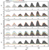 |
Fig. 7. Same as Fig. 5, but excluding all cycles after 15. |
| In the text | |
|
Fig. 8. Comparison of RMS differences returned by the various methods with that of CEA17 by considering different calibration periods. The curves are shown as the RMS difference of each method (as denoted in each panel) minus the RMS difference of CEA17 (positive and negative values mean CEA17 performs better and worse than the respective method, respectively). |
| In the text | |
|
Fig. 9. Comparison of mean differences of calibrated to original RGO data for the various methods by considering different calibration periods. The vertical dashed lines indicate the acuity threshold beyond which the respective method excludes the observer based on its quality criteria (see Sect. 2.2). |
| In the text | |
|
Fig. 10. Comparison between RGO010 and RGO000 group counts, represented as the differences between the raw data ( |
| In the text | |
|
Fig. 11. Comparison between the performance of the various cross-calibration methods on synthetic observers as a function of overlap to the original RGO data. Shown are the results for synthetic observers with acuity thresholds of 1 (a, e), 5 (b, f), 10 (c, g), and 30 (d, h) msd. The shaded surfaces mark the range due to the 100 realisations for each case of overlap, but to ease visibility are shown only for CEA17 and HoSc98. The RMS differences are computed for the annual values (left column) and the daily values (right column). The horizontal black line marks the differences if the raw data are used uncalibrated (shown only at the top panels). |
| In the text | |
Current usage metrics show cumulative count of Article Views (full-text article views including HTML views, PDF and ePub downloads, according to the available data) and Abstracts Views on Vision4Press platform.
Data correspond to usage on the plateform after 2015. The current usage metrics is available 48-96 hours after online publication and is updated daily on week days.
Initial download of the metrics may take a while.