| Issue |
A&A
Volume 699, July 2025
|
|
|---|---|---|
| Article Number | A218 | |
| Number of page(s) | 10 | |
| Section | The Sun and the Heliosphere | |
| DOI | https://doi.org/10.1051/0004-6361/202554738 | |
| Published online | 11 July 2025 | |
Advancing understanding of sunspot penumbra formation with non-linear force-free field extrapolations
1
Institute for Astrophysics and Geophysics, Friedrich-Hund-Platz 1, 37077 Göttingen, Germany
2
Institut für Sonnenphysik (KIS), Georges-Köhler-Allee 401A, 79110 Freiburg in Breisgau, Germany
3
Astronomical Institute of the Czech Academy of Sciences, Fričova 298, 25165 Ondřejov, Czech Republic
⋆ Corresponding author: This email address is being protected from spambots. You need JavaScript enabled to view it.
Received:
25
March
2025
Accepted:
8
June
2025
Abstract
Context. Although sunspots have been extensively studied, the mechanism behind the formation of penumbrae is still not fully understood.
Aims. In this work, we investigate the process of sunspot penumbrae formation from a novel approach based on the analysis of magnetic fields from non-linear force-free field (NLFFF) extrapolations aiming to identifying the key parameters driving this process.
Methods. We calculate NLFFF extrapolations from HMI/SDO data sampling the development of the active region NOAA 12757 before, during, and after penumbra formation. We analyse the resulting magnetic field inclination, magnetic field tension, and the current density evolution in the leading spot. The analysis focuses on the stable part of the sunspot, away from the AR opposite polarity.
Results. The analysis of the extrapolations has revealed that: (1) the magnetic field inclination measured at the footpoints of the extrapolated field lines agrees with the results inferred from inversions, confirming the consistency of the methodology. (2) Penumbra formation is preceded by the continuous emergence of magnetic flux as outlined by serpentine fields observed in the low layers. After emerging, these fields further rise shaping the active region field topology formed by high-lying loops. (3) The emergence of local patches of new flux is characterised by high magnetic tension and significant current densities, primarily concentrated at the protospot boundary. Both the magnetic tension and current densities gradually dissipate as the magnetic loops continue to rise. This flux emergence occurs in regions where the penumbra is not yet formed and the magnetic canopy is not yet developed. (4) With the increase of emerged flux, a magnetic canopy develops and gradually expands around the spot in unison with the forming underlying penumbra. (5) As the penumbra and canopy expand, the surrounding network field, initially present close to the spot boundary, gradually migrates outward, reaching a maximum distance of about 9 Mm. This and the rise of serpentine fields, footpointed by migrating moving magnetic features provide evidence of the connectivity between the sunspot’s core magnetic field and the surrounding network field.
Conclusions. This case study provides clear evidence that the formation of stable penumbra results from a bottom-up approach: the continuous emergence and upward rise of serpentine field lines into the corona during which a sunspot magnetic canopy develops.
Key words: Sun: atmosphere / Sun: general / Sun: magnetic fields / Sun: photosphere / sunspots
© The Authors 2025
 Open Access article, published by EDP Sciences, under the terms of the Creative Commons Attribution License (https://creativecommons.org/licenses/by/4.0), which permits unrestricted use, distribution, and reproduction in any medium, provided the original work is properly cited.
This article is published in open access under the Subscribe to Open model. This email address is being protected from spambots. You need JavaScript enabled to view it. to support open access publication.
1. Introduction
Even though sunspots have been observed and investigated for many years, some physical processes operating in sunspots require more deep understanding. The structure of a sunspot reaching full development typically shows an umbra region and a penumbra. In the umbra, the magnetic field is found to be vertical and has intensities of up to 3−4 kG (see e.g. Borrero & Ichimoto 2011, and references therein). The penumbra surrounds the umbra region and appears in observations as being composed of filamented bright structures. The penumbra is formed in a time frame of a few hours, which eludes its observation with high spatial resolution, and hosts more inclined magnetic fields than the umbra with strengths of 1−2 kG.
The research on penumbra formation became more intense with high-resolution photospheric observations (Schlichenmaier et al. 2010). From these observations, it was shown by Rezaei et al. (2012) that: (1) before the formation of the penumbra, the magnetic field in the umbra region is strong and stable; (2) at the penumbra site the magnetic field is strong and inclined, and (3) the total magnetic flux of the spot increases, owing to the coalescence of newly emerging flux around the proto-spot during its development.
From a theoretical point of view, a number of realistic 3D MHD (magneto-hydrodynamic) simulations of sunspots can reproduce most of the global properties observed in stable sunspots. The first full sunspot simulation was performed by Rempel (2012). To obtain the required inclinations of the penumbral field lines in these simulations, the horizontal field strength is artificially increased at the top boundary as also pointed out by Panja et al. (2021). A recent work Jurčák et al. (2020) on sunspot simulations shows that penumbra is driven by the subsurface structure of the magnetic field and that the artificial increase of the horizontal field strength in MHD simulations results into magnetic field properties that are not in agreement with observed sunspots. The simulations performed until present are only restrained at the photospheric level. There is no report, as far as we are aware, showing the surrounding topology of the magnetic field during a sunspot penumbra formation.
Other observational studies on penumbra formation (e.g. Shimizu et al. 2012a; Romano et al. 2013) in higher (chromospheric) layers hint towards the existence of an overlying canopy as a key ingredient for penumbra formation. Yet, this has not been proven so far. The formation of sunspot penumbrae is still under debate (see e.g. Bello González et al. 2019) and the magnetic field configuration above the photosphere has not yet been investigated. Tiwari (2012) investigated whether the magnetic fields it the photosphere adhere to linear or non-linear force-free conditions. After analysing both simple and complex sunspots, the findings indicate that photospheric sunspot magnetic fields generally align more closely with the non-linear force-free field approximation.
We applied the non-linear force-free field extrapolation (NLFFF) method (Wheatland et al. 2000; Wiegelmann 2004; Wiegelmann & Inhester 2010) to a series of HMI vector magnetograms that recorded the sunspot penumbra formation process aiming to investigate the properties of the overlying magnetic field before and during penumbra formation. The structure of the paper is as follows: in Section 2 we describe the observations, Section 3 is dedicated to the methodology description; in Section 4 we present the results of the investigation and Section 5 is reserved for the conclusions and discussions.
2. Observations
We used observations from the HMI instrument (Schou et al. 2012) onboard the SDO spacecraft (Pesnell et al. 2012) which provides continuous vector magnetograms with 12 min cadence and 1 arcsec spatial resolution.
For the selection of our observations, we searched for a pore that formed a fully developed sunspot while on the visible disc within ±30° latitude and longitude. We select the sunspot near the sun centre to be able to use the non-linear force-free field method (NLFFF) method in the Cartesian geometry. This region, within ±30° latitude and longitude, is where the magnetic field measurements are more reliable, and the Sun’s surface can be reasonably approximated as planar. To identify a suitable candidate, we examined continuum images from HMI/SDO. A pore/sunspot, part of the active region AR 12757, was observed on 26 January 2020, at the beginning of the cycle 25 when the solar activity was at its minimum. We chose this particular pore/sunspot to minimise the influence of surrounding magnetic activity on the forming sunspot.
For the analysis of the sunspot penumbra formation we used the SHARP (Spaceweather HMI Active Region Patch) HMI vector magnetograms and continuum images. The SHARP magnetograms are obtained from inversions in the Milne-Eddigton (ME) approximation with the VFISV code (Borrero et al. 2011). To have good coverage of the penumbra formation stages, we selected an observational interval of 18 hours, with a 12-minute cadence, starting at 04:12 UT when we could identify the early stage of the sunspot (pore) until 22:00 UT when the data show a fully formed sunspot. The coordinates from the Sun centre of the pore/sunspot centre spanned in longitude from 10.62° E to 0.09° W where the solar latitude was 8.42° N.
In Fig. 1, we show three snapshots of the sunspot evolution, the initial and last frame of the analysed sequence in the left and right columns, respectively. In the middle column we show the sunspot at an intermediate step of the analysed time period. The top row and middle row shows the snapshots in the continuum and magnetic field intensity, and in the bottom row we display the inclination angle obtained from the inversions. We defined the umbra and penumbra boundaries using continuum intensity where the intensities are normalised to the quiet Sun, IQS. Umbral regions are defined by a maximum intensity of 0.5 IQS, green contours in Fig. 1. The penumbral regions are defined as 0.5 < IQS < 0.95, magenta contours in Fig. 1 and brighter regions are taken as quiet-Sun.
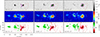 |
Fig. 1. HMI intensity maps (top row) and magnetic field strength (middle row) and magnetic field inclination (bottom row) of the AR 12757 on January 26, 2020. Magnetic field inclination is shown only in pixels with B > 150 G. Maps corresponding to the start and end times of our analysis are shown in the left and right panels, respectively. The middle panels show the active region in the middle of the analysed time period. The green and magenta contours show the umbra/penumbra and penumbra/quiet Sun boundaries, respectively. The black oval contours show the distance from the ellipse centre at r/r0 = 1, 2, 3, where r0 is the “radius” of the ellipse fitted to the penumbra/quiet Sun boundary at the end time of the analysed time period. The red dashed contours show our region of interest (ROI). The temporal evolution of a close-up of the are under study is available online. |
To analyse various physical parameters relative to the position within the sunspot, we inscribed an ellipse to the outer penumbral boundary of the sunspot once it fully developed (last frame of the analysed time period, right column in Fig. 1). The semi-minor and semi-major axes of the ellipse are approximately 9 Mm and 10 Mm, respectively. Thus, we can ascribe the radial distance with respect to the ellipse radius to all pixels within the field of view (FOV). Radial distances are shown for all frames by black contours in Fig. 1. We focus our analysis on the western part of the leading sunspot, where the evolution of the penumbra is not influenced by the interaction with the opposite polarity of the tailing magnetic field and the penumbra develops coherently in this region. The region of interest (ROI) is marked by the dashed red lines in Fig. 1.
3. Methodology
3.1. NLFFF extrapolations
For the NLFFF modelling, we used the vector component of the photospheric magnetic field from the SHARP-CEA maps. The vector B is remapped to a Carrington (CRLN/CRLT) coordinate system with cylindrical equal area (CEA) projection and decomposed into radial (Br), transversal (Bt), and longitudinal (Bp) magnetic field.
We modeled the magnetic field of the forming sunspot from the photosphere to the low corona using the non-linear force-free field (NLFFF) extrapolation method. This modelling relies on specific assumptions about the solar corona’s environment. According to the plasma-β model by Gary (2001), magnetic pressure dominates over plasma pressure, gravity effects, and kinematic ram pressure from plasma flows in the corona (Wiegelmann & Sakurai 2012). Under these conditions, the force-free field assumption is applied, where the Lorentz force vanishes, satisfying the non-linear equation j × B = 0, along with the solenoidal condition ∇ ⋅ B = 0.
To solve these force-free equations, we employ an optimization approach originally proposed by Wheatland et al. (2000) and later developed by Wiegelmann (2004) and Wiegelmann & Inhester (2010). The current version of the NLFFF optimization approach uses surface observations of all three magnetic field components as boundary conditions.
The core of the NLFFF method is minimising a scalar cost function (Ltot), which consists of multiple terms that enforce the constraints that the final solution must satisfy. These terms are designed to ensure consistency with the underlying physical assumptions. The terms of the functional are
 (1)
(1)
 (2)
(2)
 (3)
(3)
The function to be minimised is
 (4)
(4)
The computational box has an inner physical domain surrounded by a buffer zone on the top and lateral boundaries. The force-free and divergence-free conditions are satisfied if the first two terms (Eqs. (1) and (2)) are minimised to zero. wf is a boundary weight function which is set to unity in the physical domain and it decreases monotonically to zero towards the outer buffer zone (see Wiegelmann 2004, for more details). The third term (Eq. (3)) minimises the differences between the observed and modelled magnetic field at the bottom boundary. In Eq. (3), σq(r) are estimated measurement errors for the three field components q = x, y, z on S (see Tadesse et al. 2011, for more details).
In an ideal configuration, all terms (L1…L3) are minimised to zero. By using photospheric observations and considering that the assumptions of the method are not fulfilled in the entire computational domain, the final solution of the NLFFF extrapolation always has residual values in all terms of the functional. The NLFFF extrapolation method is an ill-posed and ill-conditioned problem, where measurement errors at the boundary tend to amplify with increasing height. While the force-free condition is well-satisfied in the corona, it is only partially met in the photosphere and chromosphere. According to Tiwari (2012), the force-free field condition holds within the sunspot region at the photospheric level. However, in the chromosphere, plasma pressure becomes the dominant force, making the NLFFF method less suitable for modelling this layer. Notably, the NLFFF approach considers only the magnetic field configuration and does not account for other forces or pressures.
For the calculations of the NLFF magnetic field, we used the multiscale approach. On the coarsest grid of 110 × 42 × 100 in the x × y × z directions, we use an initial potential field determined from the normal component of the HMI surface field. The solution of the NLFFF extrapolation, on all but the finest grid, is interpolated on the next grid and used as the initial condition for the extrapolation on the new grid. The final coronal field model analysed below is the result obtained on the 440 × 168 × 400 grid. At any level change, the grid size is reduced (enhanced) by a factor of two. The NLFF field reconstructions are calculated iteratively from an initial magnetic field until the field B has relaxed to a force-free state.
In total, we obtained 90 solutions of the magnetic field modelling based on the NLFFF method. In the z direction, the spatial range is [1, 1.5] Rs, and one grid point of the box is 2.6 Mm.
3.2. Magnetic tension
One of the assumptions of the NLFFF method is the force-free conditions in the solar corona, which also means that the current density J is parallel to the magnetic field B, so the Lorentz force is zero. The Lorentz force (j × B) can be defined as a sum of the magnetic tension and pressure (Eq. (5)), two competing forces that if they are in balance they fulfill the force-free condition:
 (5)
(5)
In a force-free environment, the parallel components of the magnetic tension and pressure cancel out, and the acting contributions are the perpendicular components on the B.
The magnetic tension force (Tm) acts orthogonal to B, and it can be written as kB2/4π, where k represents the curvature vector that points towards the centre of the curvature of the magnetic field line and has the expression  , where
  is the unit vector of the magnetic field (
 ). An increase in the magnetic field line curvature means an increase in the tension force.
3.3. Consistency check: HMI vs. extrapolations inclinations
The initial bottom boundary condition for the NLFFF extrapolation is the magnetic field vector obtained by Milne-Eddington inversions (VFISV, Borrero et al. 2011) of the spectropolarimetric data observed by HMI/SDO. The average inversion errors for the data used are approximately 50 G for the magnetic field strength and 6° for the magnetic field inclination (mean values of the errors over the field of view and time as determined by the inversion code VFISV). As given by Eq. (3), the discrepancy between the inferred and model magnetic field vector at the bottom boundary is one of the cost functions that is minimised during the NLFFF extrapolation. By applying a 4th-order Runge-Kutta method, we traced every field line resulting from the extrapolation to its footpoint within the FOV. We calculated the angle between the tangent of the magnetic field lines and the normal to the surface. In Figs. 2 and 3, we compare the magnetic field inclination and strength, respectively, within the outermost ellipse shown in the right panel of Fig. 1 (fully fledged leading sunspot at 22:00 UT) derived from the inversion, γinv and Binv (left panels), with the inclination and field strength of the resulting NLFFF field lines, γext and Bext, respectively (second panels from left). In the third plot (from left) of Figs. 2 and 3, we show the probability density functions (PDF) of all the pixels within the same area for the entire analysed period. For display purposes, we neglect the field’s polarity for the inclination, and thus 0° corresponds to the vertical field irrespective of its polarity and 90° to the horizontal field.
 |
Fig. 2. Comparison of magnetic field inclination from ME inversion (γinv) and from NLFFF extrapolation (γext) within the outermost ellipse marked in Fig. 1. From left to right, the first and second panels show the scatter plots of γinv and γext, respectively, as a function of radial distance from the spot centre for data from 22:00 UT (fully fledge spot). The third panel shows the probability density function of the relation between γext on γinv for all times and all pixels within the ellipse. The green colour corresponds to pixels with I/Ic < 0.5 (umbra), the magenta colour corresponds to pixels with 0.5 < I/Ic < 0.95 (penumbra), and the red colour corresponds to pixels with I/Ic > 0.95. The right-most panel shows the mean difference between the inclination values determined from extrapolations and from inversions in penumbral regions (magenta line) and umbral regions (green line). The black line shows the smoothed value for all pixels within the sunspot. |
It can be seen that in the umbra and penumbra (green and magenta colours), the inclination values are similar where γext is on average 5° to 10° more horizontal than γinv. In these areas, Bext and Binv show similar values where Bext is on average approximately 100 G stronger than Binv. Comparing the first two panels of Figs. 2 and 3, the γext and Bext in umbra and penumbra have fewer outliers compared to γinv and Binv, respectively, that is, extrapolation also smooths the distribution of inversion values.
In the quiet Sun regions, where the magnetic field strength is negligible and the field lines are not well defined, γinv is predominantly around 80° (caused by the inherent limitations of inversion codes that tend to fit noise in the Stokes Q and U signals) and NLFFF extrapolations provide γext around 90°. In these regions we obtain comparable values of Bext and Binv. Similarly to umbral and penumbral regions, Bext is approximately 100 G stronger than Binv on average.
In quiet-Sun areas, we also observe strong network fields. Those are apparent as red peaks in the scatter plots in Fig. 3, where the amplitude of the peak is higher by 200 G for Bext compared to Binv. Such peaks are difficult to identify in the scatter plots of magnetic field inclination in Fig. 2 as this parameter is more sensitive to noise than magnetic field strength. Nevertheless, γext and γinv are comparable also in these network areas as shown in Fig. 6 in Sect. 4.
In the right-most panel of Fig. 2, we show the temporal evolution of the mean difference between the inferred inclination values. It shows that NLFFF extrapolations can better fit the fully developed AR as the mean difference of inclinations is decreasing from around 7° to 3°. For this panel, we used only pixels within the sunspot (within magenta contours shown in Fig. 1). We note that the trend is not so obvious if we compare γinv and γext in the ROI. There, the difference is around 4° from the beginning of the time period analysed. Similarly, Binv and Bext also best fit during the mature sunspot stage, after the difference drops from around 130 G down to 60 G for the penumbral areas (magenta). In the umbra, the difference in value is lower, running from 80 G down to around 40−50 G.
The results of this comparison gives as confidence in the methodology used in this investigation. We are not aware of any such comparison between NLFFF results and observations in previous studies.
3.4. Tracing magnetic field lines
The extrapolations allow us to track changes in the field topology and to trace individual field lines from the protospot to the fully fledged sunspot stage. We traced two sets of magnetic field lines to analyse the evolution of the magnetic field. The first set provides a global overview of the entire computational domain, while the second focuses on a specific region of interest. For the global view, to ensure consistency and avoid bias in loop selection, we determined a set of randomly selected (x, y) footpoints, which were used as starting points for tracing magnetic field lines in each NLFFF solution. Figure 4 shows three snapshots that highlight selected 3D magnetic field lines that outline the magnetic topology of the active region at the start (04:12 UT, top panel), middle (13:00 UT, middle panel) and end (22:00 UT, bottom panel). An animation of the complete time evolution is available in the supplementary material. For the local view, we traced magnetic field lines with footpoints at different constant y-values within the ROI and for x-values ranging from 280 to 310 pixels ([140, 155] arcseconds). The same pairs (x, y) of footpoints were used for all time frames. An example of a locally traced set of loops is presented in Figure 5.
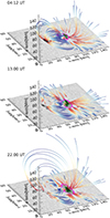 |
Fig. 4. 3D loops traced from the solution of the NLFFF extrapolation at 04:12 UT (left panel) and 22:00 UT (right panel), overplotted on the HMI magnetogram. The colour code of the loops is scaled with the height of the loops: red shows the footpoints and blue shows the highest point of the loops. |
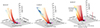 |
Fig. 5. Snapshots of the magnetic field lines in a selected area at different stages during penumbra formation. Each height step corresponds to 2.6 Mm. The colour coding represents the proximity of the field-line summit: blueish tones indicate nearby field lines that close locally, while reddish tones indicate more distant summits (‘open’ field lines connecting to the AR opposite polarity or extending beyond). |
4. Results and discussion
We follow the development of the AR 12757 leading spot for 18 hours. As seen in the intensity movies associated with Fig. 1, the sunspot develops from a protospot stage by coalescence of the nearby pores of the same polarity, similar to the process reported from high-resolution observations by Rezaei et al. (2012) and references therein.
High-resolution observations of a sunspot report a penumbra forming in segments (García-Rivas et al. 2024; Rezaei et al. 2012). In agreement with previous observations, the AR 12757 leading sunspot’s penumbra develops by sectors rather than uniformly. The first sector begins to form within the ROI. The second starts forming in the south-east of the previous. A third larger sector starts to form on the opposite (northern) side of the spot. It is noticeable that the penumbral sector starting to form last is eventually the first to reach its maximum width (see for example time 19:48 UT in the movie).
4.1. Magnetic field topology during penumbra formation
We follow the local evolution of the magnetic field topology during penumbra formation by tracing magnetic field lines in selected seed pixels, as described in Section 3.4. The ROI is selected based on the following criteria: (1) We focus on a penumbra that forms on the spot side away from the AR’s opposite polarity. With this, we avoid complex areas of intense magnetic and dynamic activity during the AR formation. This allows the study of the forming penumbra in a quiet environment, and (2) the seed pixels are selected along extended cuts across this area.
Plots of a close-up of the field lines of one of the cuts at three selected times that correspond to key moments of penumbra formation are shown in Fig. 5. The times correspond to the protospot stage (05:24 UT), forming penumbra (11:00 UT), and fully fledged penumbra (16:48 UT), respectively. Animations of the full evolution are provided as supplementary material.
4.1.1. Emergence of serpentine fields (05:24 UT).
During the protospot stage, magnetic field lines emerge at the solar surface as serpentine fields, undulating up and down, likely as a result of convective buffeting during their ascent through the sub-photospheric layers.
4.1.2. The magnetic field topology develops (11:00 UT).
After likely shedding their mass load, we observe the rise of the serpentine fields bringing new flux into the atmosphere. The continuous emergence of these rising field lines, transitioning from inclined to more vertical, gradually shapes the magnetic field topology of the sunspot in that region.
4.1.3. The sunspot magnetic field reaches equilibrium (16:48 UT onwards).
Field lines continue to further rise, with some (red-topped) connecting to the AR opposite polarity and others (blue-topped) connecting to nearby opposite polarities. At this stage, magnetic flux continues to emerge onto the solar surface, as evidenced by the appearance of new serpentine fields. However, the densely packed spot magnetic field bundle of the spot hinders the easy ascent of the new field lines. A state of equilibrium or saturation has been reached.
4.1.4. Serpentine fields and moving magnetic features (MMFs).
The footpoints of serpentine fields appear in HMI photospheric magnetograms as MMFs of both polarities and can be traced in the inclination maps of the movie associated with Fig. 1. MMFs are also apparent in Fig. 6, where the upper panel presents a time-distance plot of the azimuthally averaged HMI-inverted magnetic inclination within the ROI. Only pixels with a magnetic field strength larger than 200 G are considered in the averaging. MMFs of both polarities can be tracked as they migrate from the sunspot’s main field toward the magnetic patches of network fields. Their presence as footpoints of the serpentine fields, along with the previously described evolution of the traced field lines, provides evidence of the connectivity between the forming sunspot magnetic field and the surrounding network.
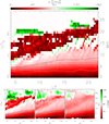 |
Fig. 6. Upper panel: Time-distance plot of the azimuthally averaged values of magnetic field inclination derived from HMI observations in the ROI marked by the dashed red lines in Fig. 1 at the photospheric level. The white and black lines outline the mean position of the umbra/penumbra and penumbra/quiet Sun boundaries, respectively. Lower panels: Same as upper panel but for the extrapolations at 0 Mm, 7.9 Mm, and 15.8 Mm. The azimuthal average of γ is only applied in pixels where B > 200 G. |
4.2. Formation and development of the sunspot magnetic canopy
Following the development of the sunspot magnetic field through the continuous emergence of field lines in the ROI (see Sect. 4.1), we now investigate in more detail the formation of the sunspot magnetic canopy and its coupling with the underlying forming penumbra.
4.2.1. Photosphere.
In the ROI, on average, the penumbra (shown in Fig. 6 as the region between the white and black lines) initially shows a length of about 1.5 Mm. It gradually extends until reaching stability at a length of 5 Mm. This penumbral length corresponds to 0.6 of the radius of the spot, a generally observed ratio found in developed sunspots (e.g. Keppens & Martinez Pillet 1996; Westendorp Plaza et al. 2001; Mathew et al. 2003; Borrero et al. 2004; Bellot Rubio et al. 2004; Sánchez Cuberes et al. 2005; Beck 2008; Borrero & Ichimoto 2011).
The plots show indications of a photospheric magnetic canopy with an average inclination of 75° developing and expanding around the spot in unison with the growth of the penumbra (outlined by the black line).
During the protospot phase, the magnetic canopy does not extend beyond the sunspot intensity boundary. It steadily expands during the development of the spot (i.e. the gathering of incoming flux and formation of the penumbra) until it reaches about 3 − 4 Mm beyond the boundary of the spot.
As the penumbra forms, we also observe a gradually increasing distance between the network field (outlined by the highly vertical fields in red and green), the sunspot’s visible boundary, and the sunspot’s magnetic canopy. Once the penumbra has fully developed in the ROI, the distance between the sunspot boundary and the network is found to be around 9 Mm. This value is comparable with the extension of the moat cell reported by Löhner-Böttcher & Schlichenmaier (2013) from a sample of 31 spots. In between the sunspot canopy and the network field, we observe migrating MMFs as described in Sect. 4.1.
4.2.2. Extrapolations.
The evolution of the magnetic field inclination at three selected heights probed by the extrapolations is shown in the lower time-distance panels of Fig. 6. A movie of the evolution at all heights up to 20 Mm is also available as supplementary material. Those allow for studying the topology of the sunspot magnetic field in the ROI at higher layers of the atmosphere. As in the photosphere, the magnetic canopy evolves as the spot gathers the incoming flux. This is expected from sunspot models, yet observational evidence is now shown here.
Starting from the sunspot centre, the magnetic funnel topology radially extends from vertical (0° to 45°) fields in the sunspot core to fields with 80° (70°) inclination at 7.9 Mm (15.8 Mm) between the sunspot and the outward-migrating network, eventually becoming more vertical (60°) above the photospheric network. This evolution shows the interaction between the sunspot funnel and the network fields: the network fields shape the edge of the sunspot funnel, turning it more vertical, while at the same time, the network magnetic field becomes more horizontal with height as it interacts with the sunspot magnetic canopy.
From high-resolution observations of a partly fledged sunspot, Lindner et al. (2023) found spectro-polarimetric signatures of a chromospheric magnetic canopy exclusive of the areas where the penumbra formed. In previous studies, Shimizu et al. (2012b) and Romano et al. (2013) had reported a chromospheric halo in areas around a protospot in which penumbra formed later on. Those halos could also be interpreted as signatures of a canopy previous to the penumbra formation as the ones presented here.
4.3. Magnetic tension
The magnetic tension force is considered to have a stabilising effect on the convective motions, by balancing the buoyancy force (Priest 1982). From the results of the NLFFF extrapolations, we calculated the tension force from the photosphere to the corona based on the equation described in Section 3.2.
In Fig. 7, we show three snapshots of the magnetic tension in the leading sunspot at the photospheric level. The complete temporal evolution of Tm is available in the movie associated with Fig. 7. From the time evolution, we observe concentrations of enhanced tension force mostly in the sunspot umbra and the inner to mid penumbra. After approximately 180 minutes (from the beginning of the studied period), we observe in the ROI an overall decrease in the tension force as the penumbra boundary extends and penumbra develops. The tension force is proportional to both the (square of the) magnetic field strength and the curvature of the magnetic field lines. A comparison with curvature values (not shown) shows that enhanced Tm values result from a combination of locally increased curvature combined with larger field strengths than those in the surroundings.
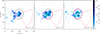 |
Fig. 7. Magnetic field tension at the photosphere at the initial state of the sunspot analysis (left panel), intermediate state at 13:00 UT (middle), and at the end of the analysis (right panel). The contours are identical to those used in Fig. 1. The temporal evolution of Tm is available online. |
Based on photospheric magnetic fields, Venkatakrishnan & Tiwari (2010) and Tiwari (2012) studied the manifestation of the vertical magnetic tension force in fully formed sunspots. Venkatakrishnan & Tiwari (2010) found that in sunspots, at photospheric level, stronger vertical tension forces are present in stronger and more vertical fields. For the penumbra region, we find a Pearson correlation value of 0.91 between the unsigned vertical magnetic field and the tension force (as defined in Sect. 3.2), and we find a poor correlation (0.42) between the unsigned vertical magnetic field and the tension force in the umbra region. It is to be noted that the vertical tension force derived by Venkatakrishnan & Tiwari (2010) is a signed parameter, while the tension force we derived (Section 3.2) is an unsigned parameter, orthogonal to the B, directed radially inward to the magnetic field line curvature.
4.4. Current density
The presence of electric currents signals a deviation from the minimum-energy, current-free (potential) configuration of the magnetic field. Consequently, free magnetic energy is directly associated with the electric currents in the solar corona. By determining the three-dimensional structure of the vector magnetic field, the vector current density can be calculated as the curl of the magnetic field. Figs. 8 and 9 show the vertical Jz and horizontal Jhor components of J, respectively. Temporal evolutions of both Jz and Jhor are provided as supplementary material. As far as we are aware, this is the first attempt to investigate the evolution of the current density during the sunspot penumbra formation.
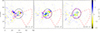 |
Fig. 8. Analogous to Fig. 7, but for the vertical current density at the photospheric level. The temporal evolution of Jz is available online. |
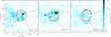 |
Fig. 9. Analogous to Fig. 7, but for the horizontal current density at the photospheric level. The temporal evolution of Jhor is available online. |
Strong vertical currents are important due to their association with the buildup of twisted magnetic structures, such as flux ropes. Strong vertical currents can suggest the formation of current sheets–thin regions where the magnetic field changes direction sharply. These current sheets are prime locations for reconnection. In the Jz component shown in Fig. 8, we observe the strongest vertical currents in the eastern part of the protospot, away from the ROI. These strong vertical currents are associated with the surrounding pores coalescing the protospot (see Fig. 1, and the associated movie). These patches of enhanced Jz are not associated with a stronger Jhor component (Fig. 9).
In the umbra, we observe a mixed current density polarity until approximately 21:00 UT, after which it stabilises, with positive Jz in the north and negative Jz in the south. The low values of the current densities suggest low magnetic field twisting (as the currents are determined by the curl of the magnetic field). This implies that the system reached a lower energy state, likely following the release of accumulated free energy. The images in the extreme ultraviolet wavelengths (not shown here) reveal a couple of eruptions originating from this active region, during which the magnetic free energy (the difference between the force-free and potential energy) is released.
In the western and northern regions of the penumbra, the negative Jz polarity predominates, although occasional small fluctuations with positive polarity occur. These two regions correspond to the stable sector (ROI), and the sector first reaching maturity (northside of the sunspot). On the western side of the studied sunspot, in the ROI, we observe lower values of Jz when compared with the eastern ones.
Strong horizontal currents are found in active regions where intense magnetic fields emerge from the Sun’s interior. Areas often coincide with locations of energy buildup before solar eruptions. The presence of strong horizontal currents can also indicate regions where magnetic reconnection might take place. During the formation of the penumbra, enhanced patches of Jh appear at various sunspot locations, mostly coinciding with the outward-moving dynamic boundary of the forming penumbra.
Examples can be seen at, for example, 04:12 UT, 06:48 UT, 07:48 UT, 11:36 UT, 13:00 UT and 19:12 UT in the animation linked to Figs. 8 and 9. They are connected to Jz bipoles with values reaching approximately half of Jhor, and to magnetic flux emergence during penumbra formation (as seen in the evolution of the magnetic inclination; Fig. 1 and associated movie).
Figure 10 shows two examples: at 04:12 UT in the top row, and 13:00 UT in the bottom row. Both exhibit enhanced magnetic tension and current density components associated with magnetic flux emergence. The inner footpoints of the emerging loop, located at the umbral boundary, show negative Jz and align with the highest Tm values detected in the sunspot. The outer footpoint, with opposite polarity to the sunspot, has positive Jz and no enhanced Tm, and is located outside the penumbra/quiet Sun boundary. The emerging loop field lines are subjected to a high curvature along their entire length (not shown), but because Tm values are proportional to B2, we obtain the highest magnetic tension at the inner footpoint. The strongest Jhor values are observed between the footpoints, indicating the loop nature of the emergence. Both J and Tm are strongest immediately after flux emergence, weakening as the field lines rise.
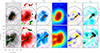 |
Fig. 10. Close-up of the protospot at 4:12 UT (top row) and 13:00 UT (bottom row) as seen in (from left to right) intensity maps, magnetic inclination, magnetic tension, magnetic field strength resulting from extrapolation, vertical and horizontal currents. All colour coding identical to previous images except for inclination, where dark green corresponds to 110 deg. The arrows point to the centre of gravity of the Tm enhancements. |
From the intensity images (Fig. 10, left column), it is clear that such flux emergence occurs in regions where we do not observe penumbral filaments and the magnetic canopy has not yet developed.
High-resolution observations of penumbra formation analysed by García-Rivas et al. (2024) showed similar indications of flux emergence at the outskirts of a protospot previous to the appearance of penumbral filaments.
In MHD simulations of sunspots carried out by M. Schmassmann (priv. comm.), flux emerges from the sub-photopsheric layers onto the solar surface, in a similar manner as indicated by the observations.
With time and the evolution of penumbrae on all sides of the sunspot studied, the observed J components weaken as the sunspot reaches a magnetic configuration closer to the potential field configuration.
Note that with HMI resolution and the simplified inversion scheme, we do not observe currents associated with the fine structure of the penumbral magnetic field (uncombed magnetic field, Solanki & Montavon 1993), where we have a weaker and horizontal magnetic field in penumbral filaments surrounded by a stronger and more vertical background field. Such currents were reported by, for example Puschmann et al. (2010) using high-resolution observations.
Based on observations, it has been determined that electric currents in well-isolated active regions (ARs) are generally balanced. At the photospheric level, currents can arise through two main mechanisms: either they emerge from below the solar surface (Leka et al. 1996) or they are generated by surface motions (Seehafer 1989). AR currents are thought to form through two primary processes: The stressing of the coronal magnetic field by photospheric and subsurface flows and the emergence of current-carrying flux from the solar interior into the corona. The first mechanism is expected to produce neutralised currents, whereas the second mechanism involves flux ropes rising through the convection zone, which are magnetically isolated and carry well-neutralised currents (Török et al. 2014). Magnetohydrodynamic (MHD) simulations have shown that significant and rapid deviations from current neutralization occur concurrently with the onset of substantial flux emergence (Török et al. 2014). Leka et al. (1996) analysed a system of five bipoles and observed the existence of an electric current carried to the photosphere before the emergence of sunspots seen in intensity. Our findings show that during penumbra formation (as part of sunspot development), local enhancements of the J components are coupled to emerging new flux. This supports the idea that electric currents locally emerge from subphotopsheric layers during sunspot formation.
Analysing the vertical current densities and magnetic gradients of a series of fully formed sunspots, Balthasar (2006) observed the opposite polarity in the values of the vertical currents, and concluded that it could be an indication of ring currents around inclined flux tubes forming the penumbra. Our observations show a continuous variation in the spatial distribution of the strong intensities pairs of positive-negative Jz polarities.
5. Conclusions
For the first time, NLFFF extrapolations were applied to SDO/HMI observations of a forming sunspot aiming to disentangle the mechanisms operating during this process. Magnetic field extrapolations confirm recent studies that indicate that the formation of a stable penumbra is a bottom-up mechanism. This mechanism is initiated by the emergence of sea-serpent fields and their subsequent rise through the atmosphere into the corona, eventually connecting to the opposite polarity of (1) the active region or (2) distant network regions.
The development of the sunspot canopy is found to occur in unison with the development of the underlying penumbra. This highlights the critical role of the overlying canopy in the formation of the penumbra by blocking the emergence and further rise of serpentine fields. This blockage provides the photosphere (and below) with the strong horizontal fields required to shape granulation into the characteristic elongated penumbral mode of magneto-convection. The analysis of the inclination of the extrapolated fields at various heights provides observational evidence of the topology of the sunspot magnetic funnel during its development, strongly influenced by the interaction with the surrounding network fields of the same polarity.
The trace of magnetic field lines reveals that as the sunspot accumulates newly emerging flux on the side facing the AR following polarity, the footpoints of the serpentine fields on the opposite spot side appear as MMFs in the inclination maps. It is also observed that the network field, originating at the outskirts of the protospot and with the same polarity, migrates outward until reaching a stable distance (around 9 Mm). As the serpentine field rises, these MMFs migrate away from the sunspot, eventually reaching the magnetic network. These together provide clear evidence of the (subphotospheric) connectivity between the developing magnetic field in the sunspot and the surrounding network.
The magnetic tension force stabilises convective motions and is strongest in the umbra and inner penumbra, decreasing as the penumbra develops. A strong correlation (0.91) is found between the vertical magnetic field and tension force in the penumbra, whereas a weaker correlation (0.42) is observed in the umbra.
Strong vertical currents are associated with twisted magnetic structures and reconnection, while strong horizontal currents coincide with energy buildup and flux emergence during penumbra formation. Observations show that local enhancements in current density are coupled with emerging flux, supporting the idea that currents originate from subphotospheric layers during sunspot development. Over time, as the sunspot evolves, the current distribution stabilises, bringing the magnetic configuration closer to a potential field state.
This pioneering study provides new insights into the formation of sunspot penumbrae. While a more extensive survey involving multiple cases will be pursued, the insights gained here significantly enhance our understanding of the key elements in the processes of sunspot and penumbra formation.
Data availability
Movies associated to Figs. 1, 5–9 are available at https://www.aanda.org
Acknowledgments
I.C. acknowledges the support of the Coronagraphic German and US Solar Probe Plus Survey (CGAUSS) project for WISPR by the German Aerospace Center (DLR) under grant 50OL2301. NBG and JJ acknowledge support by the Czech–German common grant, funded by the Czech Science Foundation under the project 23-07633K and by the Deutsche Forschungsgemeinschaft under the project BE 5771/3-1 (eBer-23 13412). JJ acknowledges the institutional support RVO:67985815. The HMI data are courtesy of NASA/SDO and the HMI science teams. This research has received financial support from the European Union’s Horizon 2020 research and innovation program under grant agreement No. 824135 (SOLARNET). We thank the referee for taking the time to carefully read the paper and for helping us improve our manuscript.
References
- Balthasar, H. 2006, A&A, 449, 1169 [NASA ADS] [CrossRef] [EDP Sciences] [Google Scholar]
- Beck, C. 2008, A&A, 480, 825 [NASA ADS] [CrossRef] [EDP Sciences] [Google Scholar]
- Bello González, N., Jurčák, J., Schlichenmaier, R., & Rezaei, R. 2019, ASP Conf. Ser., 526, 261 [Google Scholar]
- Bellot Rubio, L. R., Balthasar, H., & Collados, M. 2004, A&A, 427, 319 [NASA ADS] [CrossRef] [EDP Sciences] [Google Scholar]
- Borrero, J. M., & Ichimoto, K. 2011, Liv. Rev. Sol. Phys., 8, 4 [Google Scholar]
- Borrero, J. M., Solanki, S. K., Bellot Rubio, L. R., Lagg, A., & Mathew, S. K. 2004, A&A, 422, 1093 [NASA ADS] [CrossRef] [EDP Sciences] [Google Scholar]
- Borrero, J. M., Tomczyk, S., Kubo, M., et al. 2011, Sol. Phys., 273, 267 [Google Scholar]
- García-Rivas, M., Jurčák, J., Bello González, N., et al. 2024, A&A, 686, A112 [NASA ADS] [CrossRef] [EDP Sciences] [Google Scholar]
- Gary, G. A. 2001, Sol. Phys., 203, 71 [Google Scholar]
- Jurčák, J., Schmassmann, M., Rempel, M., Bello González, N., & Schlichenmaier, R. 2020, A&A, 638, A28 [NASA ADS] [CrossRef] [EDP Sciences] [Google Scholar]
- Keppens, R., & Martinez Pillet, V. 1996, A&A, 316, 229 [NASA ADS] [Google Scholar]
- Leka, K. D., Canfield, R. C., McClymont, A. N., & van Driel-Gesztelyi, L. 1996, ApJ, 462, 547 [NASA ADS] [CrossRef] [Google Scholar]
- Lindner, P., Kuckein, C., González Manrique, S. J., et al. 2023, A&A, 673, A64 [NASA ADS] [CrossRef] [EDP Sciences] [Google Scholar]
- Löhner-Böttcher, J., & Schlichenmaier, R. 2013, A&A, 551, A105 [NASA ADS] [CrossRef] [EDP Sciences] [Google Scholar]
- Mathew, S. K., Lagg, A., Solanki, S. K., et al. 2003, A&A, 410, 695 [NASA ADS] [CrossRef] [EDP Sciences] [Google Scholar]
- Panja, M., Cameron, R. H., & Solanki, S. K. 2021, ApJ, 907, 102 [Google Scholar]
- Pesnell, W. D., Thompson, B. J., & Chamberlin, P. C. 2012, Sol. Phys., 275, 3 [Google Scholar]
- Priest, E. R. 1982, Solar Magneto-hydrodynamics (Dordrecht: D. Reidel), 21 [Google Scholar]
- Puschmann, K. G., Ruiz Cobo, B., & Martínez Pillet, V. 2010, ApJ, 721, L58 [Google Scholar]
- Rempel, M. 2012, ApJ, 750, 62 [Google Scholar]
- Rezaei, R., Bello González, N., & Schlichenmaier, R. 2012, A&A, 537, A19 [NASA ADS] [CrossRef] [EDP Sciences] [Google Scholar]
- Romano, P., Frasca, D., Guglielmino, S. L., et al. 2013, ApJ, 771, L3 [NASA ADS] [CrossRef] [Google Scholar]
- Sánchez Cuberes, M., Puschmann, K. G., & Wiehr, E. 2005, A&A, 440, 345 [NASA ADS] [CrossRef] [EDP Sciences] [Google Scholar]
- Schlichenmaier, R., Rezaei, R., Bello González, N., & Waldmann, T. A. 2010, A&A, 512, L1 [NASA ADS] [CrossRef] [EDP Sciences] [Google Scholar]
- Schou, J., Scherrer, P. H., Bush, R. I., et al. 2012, Sol. Phys., 275, 229 [Google Scholar]
- Seehafer, N. 1989, ESA Spec. Publ., 285, 87 [Google Scholar]
- Shimizu, T., Ichimoto, K., & Suematsu, Y. 2012a, ApJ, 747, L18 [NASA ADS] [CrossRef] [Google Scholar]
- Shimizu, T., Ichimoto, K., & Suematsu, Y. 2012b, ASP Conf. Ser., 456, 43 [Google Scholar]
- Solanki, S. K., & Montavon, C. A. P. 1993, A&A, 275, 283 [NASA ADS] [Google Scholar]
- Tadesse, T., Wiegelmann, T., Inhester, B., & Pevtsov, A. 2011, A&A, 527, A30 [NASA ADS] [CrossRef] [EDP Sciences] [Google Scholar]
- Tiwari, S. K. 2012, ApJ, 744, 65 [NASA ADS] [CrossRef] [Google Scholar]
- Török, T., Leake, J. E., Titov, V. S., et al. 2014, ApJ, 782, L10 [CrossRef] [Google Scholar]
- Venkatakrishnan, P., & Tiwari, S. K. 2010, A&A, 516, L5 [NASA ADS] [CrossRef] [EDP Sciences] [Google Scholar]
- Westendorp Plaza, C., del Toro Iniesta, J. C., Ruiz Cobo, B., et al. 2001, ApJ, 547, 1130 [Google Scholar]
- Wheatland, M. S., Sturrock, P. A., & Roumeliotis, G. 2000, ApJ, 540, 1150 [Google Scholar]
- Wiegelmann, T. 2004, Sol. Phys., 219, 87 [NASA ADS] [CrossRef] [Google Scholar]
- Wiegelmann, T., & Inhester, B. 2010, A&A, 516, A107 [NASA ADS] [CrossRef] [EDP Sciences] [Google Scholar]
- Wiegelmann, T., & Sakurai, T. 2012, Liv. Rev. Sol. Phys., 9, 5 [Google Scholar]
All Figures
|
Fig. 1. HMI intensity maps (top row) and magnetic field strength (middle row) and magnetic field inclination (bottom row) of the AR 12757 on January 26, 2020. Magnetic field inclination is shown only in pixels with B > 150 G. Maps corresponding to the start and end times of our analysis are shown in the left and right panels, respectively. The middle panels show the active region in the middle of the analysed time period. The green and magenta contours show the umbra/penumbra and penumbra/quiet Sun boundaries, respectively. The black oval contours show the distance from the ellipse centre at r/r0 = 1, 2, 3, where r0 is the “radius” of the ellipse fitted to the penumbra/quiet Sun boundary at the end time of the analysed time period. The red dashed contours show our region of interest (ROI). The temporal evolution of a close-up of the are under study is available online. |
| In the text | |
|
Fig. 2. Comparison of magnetic field inclination from ME inversion (γinv) and from NLFFF extrapolation (γext) within the outermost ellipse marked in Fig. 1. From left to right, the first and second panels show the scatter plots of γinv and γext, respectively, as a function of radial distance from the spot centre for data from 22:00 UT (fully fledge spot). The third panel shows the probability density function of the relation between γext on γinv for all times and all pixels within the ellipse. The green colour corresponds to pixels with I/Ic < 0.5 (umbra), the magenta colour corresponds to pixels with 0.5 < I/Ic < 0.95 (penumbra), and the red colour corresponds to pixels with I/Ic > 0.95. The right-most panel shows the mean difference between the inclination values determined from extrapolations and from inversions in penumbral regions (magenta line) and umbral regions (green line). The black line shows the smoothed value for all pixels within the sunspot. |
| In the text | |
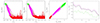 |
Fig. 3. Analogous to Fig. 2, but for magnetic field strength. |
| In the text | |
|
Fig. 4. 3D loops traced from the solution of the NLFFF extrapolation at 04:12 UT (left panel) and 22:00 UT (right panel), overplotted on the HMI magnetogram. The colour code of the loops is scaled with the height of the loops: red shows the footpoints and blue shows the highest point of the loops. |
| In the text | |
|
Fig. 5. Snapshots of the magnetic field lines in a selected area at different stages during penumbra formation. Each height step corresponds to 2.6 Mm. The colour coding represents the proximity of the field-line summit: blueish tones indicate nearby field lines that close locally, while reddish tones indicate more distant summits (‘open’ field lines connecting to the AR opposite polarity or extending beyond). |
| In the text | |
|
Fig. 6. Upper panel: Time-distance plot of the azimuthally averaged values of magnetic field inclination derived from HMI observations in the ROI marked by the dashed red lines in Fig. 1 at the photospheric level. The white and black lines outline the mean position of the umbra/penumbra and penumbra/quiet Sun boundaries, respectively. Lower panels: Same as upper panel but for the extrapolations at 0 Mm, 7.9 Mm, and 15.8 Mm. The azimuthal average of γ is only applied in pixels where B > 200 G. |
| In the text | |
|
Fig. 7. Magnetic field tension at the photosphere at the initial state of the sunspot analysis (left panel), intermediate state at 13:00 UT (middle), and at the end of the analysis (right panel). The contours are identical to those used in Fig. 1. The temporal evolution of Tm is available online. |
| In the text | |
|
Fig. 8. Analogous to Fig. 7, but for the vertical current density at the photospheric level. The temporal evolution of Jz is available online. |
| In the text | |
|
Fig. 9. Analogous to Fig. 7, but for the horizontal current density at the photospheric level. The temporal evolution of Jhor is available online. |
| In the text | |
|
Fig. 10. Close-up of the protospot at 4:12 UT (top row) and 13:00 UT (bottom row) as seen in (from left to right) intensity maps, magnetic inclination, magnetic tension, magnetic field strength resulting from extrapolation, vertical and horizontal currents. All colour coding identical to previous images except for inclination, where dark green corresponds to 110 deg. The arrows point to the centre of gravity of the Tm enhancements. |
| In the text | |
Current usage metrics show cumulative count of Article Views (full-text article views including HTML views, PDF and ePub downloads, according to the available data) and Abstracts Views on Vision4Press platform.
Data correspond to usage on the plateform after 2015. The current usage metrics is available 48-96 hours after online publication and is updated daily on week days.
Initial download of the metrics may take a while.