| Issue |
A&A
Volume 699, July 2025
|
|
|---|---|---|
| Article Number | A153 | |
| Number of page(s) | 12 | |
| Section | Catalogs and data | |
| DOI | https://doi.org/10.1051/0004-6361/202554700 | |
| Published online | 07 July 2025 | |
Magnitude-limited catalogue of unresolved white dwarf-main sequence binaries from Gaia DR3
1
Departament de Física, Universitat Politècnica de Catalunya,
c/Esteve Terrades 5,
08860
Castelldefels,
Spain
2
Institut d’Estudis Espacials de Catalunya (IEEC),
C/Esteve Terradas, 1, Edifici RDIT,
08860
Castelldefels,
Spain
3
Centro de Astrobiología (CAB), CSIC-INTA,
Camino Bajo del Castillo s/n,
28692
Villanueva de la Cañada,
Madrid,
Spain
4
Hamburger Sternwarte, University of Hamburg,
Gojenbergsweg 112,
21029
Hamburg,
Germany
5
Astrophysics Research Cluster, School of Mathematical and Physical Sciences, University of Sheffield,
Sheffield,
S3 7RH,
UK
6
Anton Pannekoek Institute for Astronomy, University of Amsterdam,
1090
GE Amsterdam,
The Netherlands
★ Corresponding author: alberto.rebassa@upc.edu
Received:
22
March
2025
Accepted:
18
May
2025
Context. Binary stars containing a white dwarf and a main sequence star (WDMS binaries) can be used to study a wide range of aspects of stellar astrophysics.
Aims. We built a magnitude-limited sample of unresolved WDMS binaries from Gaia DR3 to enlarge these studies.
Methods. We looked for WDMS with available spectra whose location in the Gaia colour-magnitude diagram bridges the gap between the evolutionary sequences of single white dwarfs (WDs) and the MS. To exclude spurious sources, we applied quality cuts on the Gaia photometry and astrometry and we fit the SED (spectral energy distribution) of the objects with VOSA (Virtual Observatory SED Analyser) to exclude single sources. We further cleaned the sample via visual inspection of the Gaia spectra and publicly available images of the objects. We re-fit the SEDs of the finally selected WDMS with VOSA using composite models to measure their stellar parameters and we searched for eclipsing systems by inspecting available ZTF and CRTS light curves.
Results. The catalogue consists of 1312 WDMS and we manage to derive stellar parameters for 435. This is because most WDMS are dominated by the MS companions, making it hard to derive parameters for the WDs. We also identified 67 eclipsing systems and estimated a lower limit to the completeness of the sample to be ≃50% (≃5% if we consider that not all WDMS in the studied region have Gaia spectra).
Conclusions. Our catalogue increases the volume-limited sample we presented in our previous work by one order of magnitude. Despite the fact that the sample is incomplete and suffers from heavy observational biases, it is well characterised. Thus, it can be used to further constrain binary evolution by comparing the observed properties to those from synthetic samples obtained by modelling the WDMS population in the Galaxy, while taking into account all selection effects.
Key words: binaries: close / stars: late-type / white dwarfs
© The Authors 2025
 Open Access article, published by EDP Sciences, under the terms of the Creative Commons Attribution License (https://creativecommons.org/licenses/by/4.0), which permits unrestricted use, distribution, and reproduction in any medium, provided the original work is properly cited.
This article is published in open access under the Subscribe to Open model. Subscribe to A&A to support open access publication.
1 Introduction
White dwarf-main sequence (WDMS) binaries are binary stars formed by a white dwarf (WD), the most common stellar remnant, and a main-sequence (MS) star. They are descended from MS binaries, whereby the primary, more massive star, had time to evolve out of the MS. Two general pathways lead to the formation of a WDMS, as we describe below.
The first one involves mass transfer interactions that usually take place once the primary becomes a red giant, or an asymptotic giant star. That is, the initial MS binary orbital separation is short enough (≲10 AU; Farihi et al. 2010) for the giant star to overfill its Roche-lobe and to transfer mass to the secondary, less massive, companion. Given that the mass transfer is generally dynamically unstable, the system is thought to evolve through a common envelope phase (Paczynski 1976; Webbink 2008) in which the core of the giant and the secondary star are surrounded by common material formed by the outer layers of the giant -that have been transferred to but not accreted by the companion - and friction considerably reduces the orbital separation; hence, we see orbital periods up to a few hours and days (Rebassa-Mansergas et al. 2008; Nebot Gómez-Morán et al. 2011). With respect to WDMS that have orbital periods as long as ≃1000 days are also suggested to be the outcome of common envelope evolution (Yamaguchi et al. 2024), with stable non-conservative mass transfer being the alternative evolutionary path for such long-period systems (Hallakoun et al. 2024; Garbutt et al. 2024). It is expected that these post-common envelope binaries account for approximately 25% of the initial MS binaries (Willems & Kolb 2004).
The second scenario, encompassing the remaining ≃75% of the cases, does not involve mass transfer episodes, since the initial MS binary orbits are wide enough to avoid them; consequently, the primary star evolves as a single star would. In these cases, the orbital periods of the WDMS binaries are of the order of hundreds to thousands of days.
Both the case of wide WDMS binaries that evolved similarly to isolated stars and that of post-common envelope binaries, these systems have been extremely valuable for tackling a broad range of issues. For instance, since the WD in wide WDMS binaries can be used to measure stellar ages, studies of such systems have helped constrain the age-metallicity relation (Rebassa-Mansergas et al. 2016a, 2021a) and the age-velocity dispersion relation (Raddi et al. 2022) in the solar neighbourhood, as well as the age-activity-rotation relation of low-mass MS stars (Rebassa-Mansergas et al. 2013, 2023; Chiti et al. 2024). They can also be used to test the WD mass-radius relation (Arseneau et al. 2024; Raddi et al. 2025) and the initial-to-final mass relation (Zhao et al. 2012; Barrientos & Chanamé 2021). On the other hand, close post-common envelope binaries allow for constraints to be placed on the efficiency of the common envelope ejection (Zorotovic et al. 2010; Camacho et al. 2014; Cojocaru et al. 2017; Grondin et al. 2024), the mass-radius relation of WDs (Parsons et al. 2017), low-mass MS stars (Parsons et al. 2018), and even brown dwarfs (Parsons et al. 2025) and sub-dwarf stars (Rebassa-Mansergas et al. 2019) via analyses of eclipsing systems, origins of low-mass WDs (Rebassa-Mansergas et al. 2011), angular momentum losses due to magnetic braking (Schreiber et al. 2010; Zorotovic et al. 2016), and origins of magnetism in WDs (Marsh et al. 2016; Schreiber et al. 2021).
The first large catalogue of ≃3200 WDMS binaries was built thanks to the mining of the Sloan Digital Sky Survey (SDSS; Eisenstein et al. 2011) spectroscopic database (Rebassa-Mansergas et al. 2012, 2016b), closely followed by the spectroscopic catalogue of ≃900 additional systems (Ren et al. 2018) from the Large Sky Area Multi-Object Fiber Spectroscopic Telescope (LAMOST; Cui et al. 2012). Since these samples are largely affected by selection effects, in particular, by the fact that earlier type than M companions outshine the WDs in the optical (Rebassa-Mansergas et al. 2010), efforts have been placed to combine ultraviolet photometry with optical photometry and/or spectroscopy that allowed for the identification of thousands of WDMS binaries containing F, G, and K companions (Parsons et al. 2016; Rebassa-Mansergas et al. 2017; Ren et al. 2020; Anguiano et al. 2022; Nayak et al. 2024; Sidharth et al. 2024).
A potential issue from the above studies is that they are all magnitude-limited, which makes it difficult to unveil the underlying population unless population synthesis studies are taken into account (Davis et al. 2010; Toonen & Nelemans 2013; Torres et al. 2022). In this sense, the astrometry and photometry provided by the Gaia satellite (Gaia Collaboration 2018, 2023) allow us to mitigate this effect, as it became possible to build the first volume-limited sample of 112 well-characterised candidates within 100 pc from the early data release 3 (Rebassa-Mansergas et al. 2021b). In this analysis, we defined a region in the Gaia Gabs versus GBP - GRP diagram to exclude single WD and MS stars and derived the WD and MS stellar parameter distributions, which clearly differed from those obtained from magnitude-limited samples. Moreover, a direct comparison with the parameter distributions obtained from numerical simulations that reproduced the Gaia population in the Galaxy provided additional valuable insight into binary star formation and evolution (Santos-García et al. 2025). Unfortunately, despite being a volume-limited sample, the Gaia catalogue was revealed to be highly incomplete, as most of the WDMS binaries are expected to have Gaia colours very similar to those of MS stars (Santos-García et al. 2025), which had been excluded from the analysis. As mentioned above, these systems are difficult to identify since the MS companions outshine the WDs in the optical. A promising way to move forward is to make use of artificial intelligence algorithms to differentiate among single MS stars and WDMS binaries via the analysis of available Gaia spectra from its data release 3 (DR3; Echeverry et al. 2022; Li et al. 2025; Pérez-Couto et al. 2025).
In this work, our motivation is to build up the Gaia WDMS binary sample we presented in Rebassa-Mansergas et al. (2021b). However, we have not implemented any distance cut, opting instead to maintain the focus in the bridge region of the Gaia colour-magnitude diagram (CMD) between single WD stars and single MS stars. This study is specifically aimed at providing a magnitude-limited and well-characterised sample from Gaia that can be directly compared to the output of numerical simulations, such as those we implemented in Santos-García et al. (2025). This will allow us to derive further constraints on binary evolution theory.
In Section 2, we introduce the WDMS binary sample. In Section 3, we explain our approach to deriving their stellar parameters. In Section 4, we compare our sample to other works in the literature. In Section 5, we identify eclipsing WDMS among our objects. We present our conclusions in Section 6.
2 The WDMS sample
We essentially followed the same criteria as Rebassa-Mansergas et al. (2021b) to build the WDMS binary sample from Gaia DR3 (Gaia Collaboration 2023). Specifically, we considered all objects in the intermediate region between single WD and single MS stars in the Gaia colour-magnitude diagram with parallax over the error and the G, GBP, GRP flux over error parameters greater than 10. However, in this work we did not impose any distance limit and we focussed the search on objects with available Gaia spectra. As we will see later, this condition (i.e. having available Gaia spectra) affects the completeness of our catalogue. However, it is required since we intend to measure the stellar parameters of the identified candidates from these spectra. Moreover, visual inspections are of great help in confirming the binary nature of the candidates via the identification of the two components in the available spectra. This process resulted in 126 787 selected sources, as illustrated in the top left panel of Figure 1.
To reduce contaminants (defined as sources that are not WDMS stars) from our selected candidates, we first applied a condition on the excess factor parameter provided by Gaia. This parameter is defined as C = (FBP + FRP>)/FG (Evans et al. 2018), where F denotes flux in the Gaia bands, and it is expected to be close to 1. Thus, any object with deviations from C = 1 may be associated to internal calibration issues. It should be emphasised that one of the possible causes for having a large excess factor is binarity, that is, based on Gaia reporting two sources that form a partially resolved system. As noted by Riello et al. (2021), C is colour-dependent and so, they defined C* = C − f (GBP, GRP), where the function, f, provides the expected excess at a given colour. In other words, by correcting the expected excess, any object with a |C*| value larger than zero can be considered as a potential source affected by calibration issues. It depends on the user’s choice to be as restrictive as necessary to exclude such sources. To that end, we followed the same approach as Rebassa-Mansergas et al. (2021b) and removed all sources with:
 (1)
(1)
 (2)
(2)
 (3)
(3)
This cut reduced the WDMS candidates to 82 021. It should be noted that these cuts are different from the traditional criteria suggested by Riello et al. (2021), which is based not only on the |C*| value but also on its deviation, σ. Thus, the user may exclude objects by simply applying a |C*| > Nσ cut by fixing a value of N. However, even when using N = 5, which is expected to be a largely conservative cut (meaning that most of the excluded sources should indeed be associated to spurious data), we ended up excluding clear WDMS binaries from the sample. In fact, any cut in the excess noise will unavoidably exclude real WDMS, thus affecting the completeness of the final sample. This issue is discussed in Section 4.
So far, we have only applied one constraint to the Gaia astrometry, excluding objects with parallax relative errors larger than 10%. Thus, an additional way to further exclude contaminants from our list is by removing objects associated with bad astrometric solutions. In particular, Gaia provides three parameters that can be used for such purpose (Lindegren et al. 2012): the re-normalised unit weight error (RUWE), which should be near 1.0 for point sources that are well fitted by a single-star model to their astrometric observations; the astrometric_excess_noise parameter, which quantifies the agreement between the observations of a given object and the best-fit astrometric model; and the astrometric_excess_noise_sig parameter, which gives the significance of the astrometric_excess_noise. It has been suggested in Gaia reporting that objects with RUWE > 1.4, astromet-ric_excess_noise > 2 or astrometric_excess_noise_sig > 2 may have issues with their astrometric solutions. Since larger than canonical values of RUWE are also possible due to binarity, we adopted all sources from our list with RUWE values smaller than 3, instead of 1.4. This is justified by looking at Figure 4 (topleft panel) of Belokurov et al. (2020), where less than 5% of the 801 spectroscopic binaries considered have RUWE values larger than 3. In the same way, to avoid missing possible binaries, we excluded objects satisfying astrometric_excess_noise > 3 & astrometric_excess_noise_sig > 3, rather than the canonical value of 2. As a consequence, the number of WDMS binaries in our list was further reduced to 62 386 (see the top right panel of Figure 1). In more than 99% of the cases, the sources were excluded due to the RUWE condition, whilst the rest of objects had a RUWE value smaller than 3, but large values of both astrometric_excess_noise and astromet-ric_excess_noise_sig. This means that our cuts in these last two parameters are basically irrelevant. In Section 4, we discuss the impact of the adopted RUWE cut in the completeness of our catalogue.
It is worth noting that there are more Gaia parameters that users can potentially explore to exclude possible contaminants, such as astrometric_sigma5d_max1 (see e.g. Gentile Fusillo et al. 2019), the astrometric fidelity parameter able to classify spurious data (Rybizki et al. 2022), or even alternative quantities such as the local unit weight error defined by Penoyre et al. (2022). However, we do not implement further quality cuts in astrometry and proceed in reducing the number of contaminants (in particular, single sources expected near the locus of single WD and MS stars) as follows.
We used GaiaXPy to convert the Gaia spectra of each source into synthetic Javalambre Physics of the Accelerating Universe Astrophysical Survey (J-PAS; Marín-Franch et al. 2012; Benitez et al. 2014) photometry, which consists of 57 filters continuously sampling the spectrum between 3700 and 9200 Å, thus obtaining their spectral energy distributions (SEDs). We then fitted the resulting SEDs using the Virtual Observatory SED Analyser (VOSA; Bayo et al. 2008)2 tool. In the fitting process, we only took into account those points in the SED with relative flux errors less than 10%, and all data above 4000 Å, since the signal-to-noise ratio below this value is generally substantial. This implied 1004 objects were excluded simply because they did not have enough reliable points in their SEDs. Moreover, we adopted the geometric distances for each source from Bailer-Jones (2023) and the extinction from the 3D maps of Lallement et al. (2014), but we did not use upper limits in the fits. In a first step, we used the CIFIST (Allard et al. 2013) grid (effective temperatures between 2200 and 7000 K, surface gravities between 4.5 and 5.5 dex, typical values for MS stars, and solar metallic-ity) to exclude 37 712 objects with χ2 fit values less than 10. In 99.5% of these cases, the corresponding visual goodness of fit Vgfb3 was less than 2, with a maximum value of 7.2. Since Vgfb values of less than 15 are usually taken as a validation for a good fit, these excluded objects should indeed be very likely single MS stars, possibly affected by extinction. It is worth noting that we initially applied a Vgfb < 15 cut to filter out single MS star candidates; however this resulted in a non-negligible fraction of excluded WDMS binaries and, as a consequence, we opted for the approach described above. In a second step, we fitted the remaining 24 674 sources with the Koester (2010) model grid of hydrogen-rich WDs (effective temperatures between 5000 and 40 000 K and surface gravities between 6.5 and 9.5 dex). We excluded 10 769 sources, very likely single or double4 WDs, with χ2 fit values less than 10, which correspond to Vgfb values of less than 3 in 98% of the cases, with a maximum value of 8.7. After this exercise, we were left then with 13 905 WDMS binary candidates in our list (see bottom -left panel of Figure 1).
We proceeded to visually inspect the Gaia spectra of the 13 905 candidates, which resulted in the identification of 1312 genuine WDMS binaries, 155 cataclysmic variables (which we identify as objects with spectra that display prominent and broad Balmer emission lines arising from the accretion disk) and 12 438 other sources. Most of these other sources were single, hot WDs and low-mass, low-metallicity sub-dwarfs according to their Gaia spectra. Given that the WD Koester (2010) grid and the Allard et al. (2013) CIFIST grid in VOSA do not include WD model spectra hotter than 40 000 K or low-metallicity stars (i.e. only solar abundances are included), respectively, it is not surprising that these objects were not previously considered as single stars; therefore, they had not previously been excluded. It is also worth noting that the visual classification of WDMS relies on the identification of both stars in the spectra, which is challenging if one of the components dominates the SED. This problem is worsened due to the low resolution of the Gaia spectra. As a consequence, this process is biased against the identification of WDMS with mild blue or red excess in their spectra. In Section 4 we will evaluate how these issues affect the completeness of our sample. Example spectra of a WDMS binary, a cataclysmic variable, a single hot WD and a single low-metallicity subdwarf star can be seen in Figure 2. We note that these identified CVs are not included in our WDMS catalogue, since we are focussing on non-accreting binaries. However, it is, of course, plausible that some WDMS in our sample could be detached CVs crossing the period gap.
To finalise, we visually inspected the Pan-STARSS g-band and POSS/DSS blue and red images of our objects by eye and flagged 72 objects that are possibly contaminated by the presence of bright nearby stars. Specifically, these are candidates for not being real WDMS binaries, but contaminated stars by the flux of nearby sources. Two examples are shown in Figure 3.
A summary of the different cuts we have applied, including the fraction of excluded objects, is provided in Table 1. An excerpt of the full 1312 WDMS binary catalogue is included in Table 2. The full table is is available at the CDS.
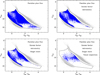 |
Fig. 1 Results of our criteria imposed on the Gaia date release 3 data base to select WDMS binaries (see details in Section 2). Top-left: 126 787 sources within the WDMS binary region defined by the black solid lines (Rebassa-Mansergas et al. 2021b) shown in blue with the available spectra and satisfying parallax and flux relative errors above 10%. The gray dots illustrate the expected location of single WD and MS stars. Top-right: same as top-left, after applying our excess factor and astrometry (RUWE; astrometric_excess_noise and astrometric_excess_noise_sig) cuts, which leaves 62 386 objects. Bottom-left: same after excluding single stars using VOSA, leaving 13 905 candidates. Bottom right: final catalogue of 1312 WDMS binaries after visual inspection of the Gaia spectra. |
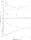 |
Fig. 2 Example spectra of a WDMS binary (top, Gaia ID 1057463111970047488. Note: in this work, we use the DR3 IDs), a cataclysmic variable (middle top: Gaia ID 3703726255561754880), a hot WD (middle bottom: Gaia ID1060659289192635904) and a low-mass low-metallicity subdwarf as revealed by the broad absorption feature at ~7000 Å (bottom: Gaia ID 1048217078174314496) arising from the visual inspection of the Gaia spectra. |
3 Stellar parameters
In this section, we attempt to derive the stellar parameters of the 1312 WDMS binary candidates. To that end, we first use the two-body fit implemented in VOSA. In this case, we complemented the Gaia J-PAS synthetic photometry with Galaxy Evolution Explorer (GALEX; Bianchi et al. 2017), Two Micron All Sky Survey (2MASS; Skrutskie et al. 2006), and Wide-field Infrared Survey Explorer (ALLWISE; Wright et al. 2018) photometry associated with good quality flags and avoiding upper limits in the fit. In the matching process, we took into account the Gaia proper motions of the targets to compute the position in the epoch 2000 and applied a search radius of 5 arcsec.
We used the low-mass star CIFIST and the hydrogen-rich WD models in the fit, which provided the bolometric luminosities (Lbol = 4πD2Fbol, where D is the distance to each target and Fbol is the bolometric flux5), effective temperatures (from the best-model fit in the grids after re-scaling the flux), and radii (both from the flux scaling factors of both components and the Stefan-Boltzmann equation) for the two components. We subsequently derived the WD surface gravities interpolating the effective temperatures and radii in the hydrogen-rich cooling sequences from La Plata (Althaus et al. 2013; Camisassa et al. 2016, 2019). Finally, we obtained the WD masses from the well-known relation g = GM/R2, where M and R are the mass and the radius, G is the gravitational constant, and g is the surface gravity (note: we obtained log g from the cooling sequences).
We visually inspected the two-body fits to evaluate the validity of the results obtained. It became obvious that in the cases where the secondary star dominates the SED, it was not possible for VOSA to find a combination of models that satisfactorily sampled the observed SEDs due to the lack of points available at blue wavelengths. As a consequence, even when the combination of models matched the observed data, we considered most of the results as unreliable since the WDs typically piled up at too low effective temperatures (5000-7000 K) as compared to those from the secondary stars (2800-3000 K). Such low-luminosity WDs would not be visible in the optical against such M star companions. An example is shown in the top panel of Figure 4. To compensate for the intrinsically low bolometric fluxes (and luminosities) of the WDs, there is a tendency for VOSA to yield large radii to those objects, which translates into very low WD masses. This likely explains the excess of extremely low-mass WDs identified in Rebassa-Mansergas et al. (2021b). In Brown et al. (in prep.) we will discuss in detail these issues, but we advance here that all fits resulting in WD effective temperatures of less than 10000K should be taken with caution. In other words, the SEDs of WDMS with dominating MS companions have few available points at blue wavelengths in their SEDs, where the WDs are expected to contribute most. As a consequence, the WD parameters tend to be unreliable. Having available GALEX photometry helps to mitigate this effect. However, the visual inspection of the fits also revealed that in some cases, the best-fit WD model failed at sampling the GALEX photometry (see the middle panel of Figure 4).
Due to the reasons outlined above, we only considered as reliable fits those with WD effective temperatures larger than 10 000 K, WD masses higher than 0.35 M⊙ and with the bestfit WD model matching the GALEX data (when available). An example is illustrated in the bottom panel of Figure 4. This resulted in 435 WDMS binaries with reliable fits. The distribution of WD effective temperatures, surface gravities and masses, and secondary star effective temperatures are shown in Figure 5.
Most WDs have effective temperatures between 12 000 and 17 000 K, with a long tail towards higher temperatures, as it is expected from a magnitude-limited sample (see e.g. Rebassa-Mansergas et al. 2010). The WD masses peak at ≃0.5 M⊙ and the surface gravities at log g ≃7.8 dex, in agreement with the volume-limited sample presented in Rebassa-Mansergas et al. (2021b). In that paper, we argued these peaks are lower than the canonical values of ≃0.6 M⊙ and 8 dex, presumably due to the fact that unresolved WDMS binaries within 100 pc are likely post common-envelope binaries, which tend to contain low-mass WDs (Rebassa-Mansergas et al. 2011). As we show in Section 5, our sample may indeed have a large fraction of post-common envelope systems, which is also expected in a magnitude-limited sample since low-mass WDs are more luminous for a fixed effective temperature (see Rebassa-Mansergas et al. 2011, for a discussion on how this effect affects the SDSS WDMS sample). However, it is also worth noting that Santos-García et al. (2025) offered evidence that ≃30% of the Gaia WDMS in Rebassa-Mansergas et al. (2021a) passed through a common envelope phase; this is a fraction that is presumably similar to what is seen for the current sample (although it could be even smaller due to the larger distances considered). Therefore, the peak at lower WD masses might also be related to the same issue with the two-body fits in VOSA mentioned above, which tends to yield lower masses than expected.
In the middle and bottom panels of Figure 6, we compare the WD surface gravities and effective temperatures, respectively, of 54 objects with reliable VOSA fits that also have such values derived from available SDSS spectra (Rebassa-Mansergas et al. 2016b). It becomes obvious that not only the surface gravities (and, hence, the masses), but also the effective temperatures derived in this work seem to be systematically lower than those obtained fitting the much higher resolution SDSS spectra. This effect may be related to reddening. Even though extinction is taken into account in the VOSA fits, it could affect the WDs more than their companions since they are bluer.
The secondary star effective temperatures are mainly concentrated between 2700 and 3400 K, with a peak at around 3200 K, which corresponds to M dwarfs of spectral types M3-M6 (Rebassa-Mansergas et al. 2007). This is in line with our expectations, since WDMS with earlier and later spectral type companions would tend to fall out of our regions of study.
The same pattern is observed when considering all WDMS binaries in the sample, including those objects with WDs cooler than 10 000 K and less massive than 0.3 M as indicated by their VOSA WD fits. We consider this as an indicator that the secondary star fits from VOSA are more reliable than those obtained for the WDs. Indeed, when comparing these temperatures with those obtained from the SDSS spectra for the 54 common objects with derived parameters6, we find that for only 12 objects (≃22% of the cases) the differences are of more than 150 K. The most dramatic discrepancy is for five objects with effective temperatures higher than 3700 K as derived from their SDSS spectra, which are considered to be much cooler according to the VOSA fits. In these cases, the temperature difference ranges from 500 to 1100 K.
We conclude this section by emphasising that the stellar parameters obtained from the VOSA two-body fits are generally reasonable and reliable for the secondary stars. Conversely, the WD parameters should only be considered as reliable for certain ranges (effective temperatures larger than 10 000 K and masses higher than 0.3 M⊙) and, especially, when GALEX photometry is available. That is, in those cases where the secondary star dominates the SED, too few photometric points are available in the blue, where the WDs make up a substantial contribution. As a consequence, the WD parameters obtained from the fit are subject to substantial uncertainties. The stellar parameters for each target with visually acceptable two-body fits are included in Table 2.
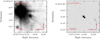 |
Fig. 3 Example images illustrating WDMS candidates (red squares) for being contaminated by the presence of nearby sources. Left panel: POSS/DSS blue image of Gaia ID 2055951194776633600. Right panel: Pan-STARSS g-band image of Gaia ID 2776554794743195648. |
WDMS selection process from our initial sample to the final catalogue.
Excerpt from the Gaia WDMS binary catalogue.
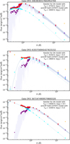 |
Fig. 4 Example of two-body VOSA fits. The top panel shows a typical MS-dominated WDMS binary in our sample. The combination of models (purple for the secondary star and cyan for the WD) seem to fit relatively well the observed data (red dots). However, the effective temperature of the WD is too low. Clearly, such a low-luminosity WD would not be seen against a 3000 K secondary M star. The middle panel illustrates an example of a bad fit, especially in the ultraviolet range. The bottom panel shows what we consider a good fit, where the models match the observed data at all wavelengths. |
4 Comparison with other WDMS binary samples
In this section, we compare our WDMS binary catalogue with other published samples from Gaia For completeness, we also compare our catalogue to the largest spectroscopic sample of WDMS binaries prior to Gaia namely, from SDSS. We also use the results of the comparisons to estimate the completeness of our sample.
We note that we do not include a comparison with Sidharth et al. (2024) since their Gaia WDMS binaries are located in the WD locus and they were therefore excluded by our selection criteria. In the same way, we do not compare our catalogue with the sample of Gaia astrometric binaries from Shahaf et al. (2024) since these objects are mainly located in the MS, therefore also outside of our region of study.
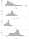 |
Fig. 5 Distribution of WD effective temperatures, surface gravities, masses, and secondary star effective temperatures derived from 435 WDMS binaries with reliable VOSA two-body fits, shown from top to bottom. |
4.1 Comparison with Rebassa-Mansergas et al. (2021b)
The present work is aimed at enlarging the volume-limited sample we provided in Rebassa-Mansergas et al. (2021b). Here, we check whether or not the 112 WDMS candidates in that sample are included in our new catalogue. Of the 112 sources, 84 have Gaia DR 3 spectra and 65 are common objects. Of the remaining 19 candidates, 5 and 6 are now classified in this work as single MS stars and single WDs, respectively, while performing the VOSA fits to their synthetic J-PAS SEDs (Section 2). We repeated the fits including GALEX, 2MASS and WISE photometry and found the same results except for two objects: Gaia ID 1900545847646195840 and Gaia ID 5490140356700680576, which display near infrared excess arguably from a low-mass companion that requires confirmation. Hence, the discrepancy between the results obtained here and those in Rebassa-Mansergas et al. (2021b) for these objects is due to the improved sampling of the optical SEDs used in this work (57 points), compared to the considerably fewer optical points used in Rebassa-Mansergas et al. (2021b); the other 8 objects are considered as a cataclysmic variable (1), as single WDs (2) or as single MS stars (5) after visual inspection of their Gaia spectra. It is also worth noting that our new catalogue includes 31 WDMS binary candidates within 100 pc that were not included in Rebassa-Mansergas et al. (2021b). In all except 8 cases the visual inspection of the 31 spectra revealed one of the two components to dominate most of the flux in the optical, systems that challenge identification by any method. The topleft panel of Figure 7 provides a confusion matrix illustrating the level of agreement between the catalogues.
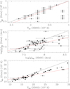 |
Fig. 6 Comparison among the WD effective temperatures (bottom) and surface gravities (middle) as well as MS star effective temperatures (top) for 54 WDMS binaries with VOSA reliable two-body fits and spectroscopic parameters derived from SDSS spectra. The black dashed lines indicate the one to one relation, whilst the red dashed lines are linear fits to the data. Note: in the top panel, values above 3700 K in the horizontal axis were not considered. |
4.2 Comparison with Nayak et al. (2024)
Nayak et al. (2024) provided a sample of 257 WDMS binaries within 100 pc by means of combining optical with ultraviolet data. This allowed us to identify WDMS binaries in the MS locus of the Gaia Gabs versus GBP - GRP diagram, with 28 of their sources falling in our region of study and 21 with Gaia spectra. Of the 21 targets, 17 are in our list, 3 are associated to a large excess and one we consider a cataclysmic variable. The top-right panel of Figure 7 provides the corresponding confusion matrix illustrating the level of agreement between the catalogues.
4.3 Comparison with Li et al. (2025)
Li et al. (2025) provided a catalogue of ≃30 000 WDMS binaries from Gaia data release 3. They used artificial intelligence neural networks to select them among the millions of available Gaia spectra. The advantage of their approach is that it allowed them to identify systems not only in the WDMS bridge between WDs and MS stars, but also outside this region. Thus, their work introduces a new methodology for identifying WDMS that can potentially reduce observational selection effects.
We compared our sample of 1312 WDMS with their list in this section. Of their 30 000 sources, 3769 are within our WDMS binary region and 962 are common objects. This means there are 2807 WDMS binary candidates in their list that we do not have and 350 candidates from our list that they do not have. Figure 7 (bottom-left) illustrates the corresponding confusion matrix between the catalogues.
We visually inspected the 2807 objects from Li et al. (2025) that were not in our list and identified 111 as WDMS. These objects were selected by our initial parallax and flux cuts, but were excluded because of large excess factor (82 sources) and uncertain astrometry (29 sources). The remaining 2696 objects were not considered by us as WDMS binaries according to our visual inspection, but they were flagged as such by the artificial intelligence neural network. Indeed, many of the spectra are virtually identical or closely resemble those of typical single MS stars and WDs and our human inspection was unable to confirm or disprove the WDMS classification. It is therefore very possible that several of those are indeed WDMS binaries. However, we also found 35 cataclysmic variables among the 2696 sources and many spectra that are difficult to interpret as representative of the WDMS binary population (see a couple of examples in Figure 8). We consider this to be likely because Li et al. (2025) did not visually inspect the spectra of their 30 000 WDMS binary candidates to exclude objects from their list.
The 350 objects that are included in our catalogue, but not in Li et al. (2025) all show the typical features of WDMS binaries in their spectra, with both components visible. Li et al. (2025) did not apply any cut in excess factor nor astrometric_excess_noise to their sample, only on RUWE. However, the RUWE values of the 350 sources are generally not too large (<≃1.5) and we have not found a clear reason why these objects were missed in their analysis.
4.4 Comparison with the SDSS WDMS binary catalogue
The spectroscopic catalogue of WDMS binaries from SDSS contains 3287 objects (Rebassa-Mansergas et al. 2016b), of which 316 have Gaia spectra and pass our parallax and flux relative error cuts of 10% (Section 2), with 140 in our final sample. Of the 176 that we do not have, 62 were excluded due to a large excess factor, 4 because they had large RUWE values, and 6 because they did not have enough points for reliable VOSA fits; in addition, 86 and 5 because they had χ2 values smaller than 10 when fitting them with VOSA using WD and low-mass star CIFIST models, respectively, and, thus, they were considered single objects; finally, another 13 were excluded because the visual inspection of their Gaia spectra did not reveal clear features of both components. We also visually inspected the 86+5 objects that we considered single objects based on their single-body VOSA fits and found the same issue; namely, their Gaia spectra did not reveal clear features of both objects. This is an observational bias related to the low resolution of Gaia All these objects reveal mild blue or red excess in the higher resolution SDSS spectra that are not featured in the Gaia spectra. Two examples are shown in Figure 9. It is worth noting that just one of the 91 WDMS that we characterised as individual sources based on their VOSA χ2 values has been included in the sample of Li et al. (2025), which indicates the neural networks also struggle to find such objects, especially those with dominant WD primaries.
In the bottom-right panel of Figure 7, we show the confusion matrix illustrating the level of agreement between our catalogue and the SDSS sample.
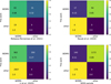 |
Fig. 7 Confusion matrices representing the level of agreement between our catalogue and other samples: Rebassa-Mansergas et al. (2021b) at the top-left, Nayak et al. (2024) at the top-right, Li et al. (2025) at the bottom-left, and the SDSS WDMS sample at the bottom-right. The values within the matrices indicate the number of targets falling in each category and the percentages respect to the total number of objects in each row. In particular, the top-left cells in each matrix indicate the number and fraction of common objects, whilst the diagonal cells indicate the number of objects (and fractions) missed (or not included) by the corresponding works. |
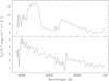 |
Fig. 8 Example spectra of WDMS binaries in the list of Li et al. (2025) that we do not consider as such. Gaia source IDs are 767397543537053312 (top) and 5952567592693723904 (bottom). |
4.5 Completeness of the catalogue
From the analysis in the previous sections, we were able to identify several important issues that limit the completeness of our WDMS binary catalogue, defined as Ncat/Ntot, where Ncat is the number of WDMS binaries in our catalogue and Ntot is the total number of observable WDMS binaries within the considered region of the Gaia Gabs versus GBP - GRP diagram. Ideally, Ncat/Ntot should be close to 1.
To begin with, not all the WDMS binaries with Gaia photometry and astrometry have spectra. For example, of the 3287 SDSS WDMS binaries, 3089 have Gaia photometry and astrometry, but only 316 have Gaia spectra (Section 4.4). In the 100 pc samples from Nayak et al. (2024) and Rebassa-Mansergas et al. (2021b), 21 out of 28 and 84 out 112, respectively, have Gaia spectra (Sections 4.2 and 4.1). Thus, at 100 pc the fraction of WDMS with Gaia spectra seems to be ≃75%, and drops significantly to ≃10% for distances as large as 1.5 kpc (approximately the maximum distance at which the SDSS WDMS binaries are located; Rebassa-Mansergas et al. 2010).
In addition, in Section 4.3 we identified 111 WDMS binaries from Li et al. (2025) that are not in our catalogue because of the excess factor and astrometry cuts applied in Section 2. In the same way, 66 SDSS WDMS binaries with Gaia spectra are not in our final list because of the same reasons (Section 4.4). Since our sample consists of 1312 sources and 177 targets are confirmed WDMS stars that did not make it to our catalogue, this means that we missed at least ≃12% of the WDMS binaries. A further complication is the fact that it becomes increasingly more difficult to identify WDMS binaries with mild blue or red excess in their optical spectra due to the low resolution of Gaia. As mentioned in Section 4.4, 91 SDSS WDMS binaries of such characteristics were excluded from our sample since we considered them as individual sources based on the results from the VOSA fits. Knowing that our final sample is Ncat = 1312 and recalling that Ntot is the total number of observable WDMS within the considered region, then:
 (4)
(4)
where fspec is the fraction of expected WDMS with Gaia spectra (≃0.1; this is a lower limit since the fraction depends on the distance considered), fcuts is the fraction of expected WDMS with Gaia spectra that we recovered after applying our cuts in astrometry and excess factor (≃0.88; this is an upper limit since at least a fraction of 0.12 are expected to be missed, as discussed above), and fvis is the fraction of WDMS with Gaia spectra satisfying our quality cuts that we expect to display both components (or at least significant blue or red excess) in their spectra (≃0.6). We note that 40% of the SDSS WDMS satisfying our quality cuts do not show both components in their low-resolution Gaia spectra and some are even considered as single objects when performing the VOSA fits (see Section 4.4).
From the above fractions and Equation (4), we derived a value of Ntot =24 848, which sets a lower limit for the completeness Ncat/Ntot of ≃5% for our catalogue - or ≃50% if we consider WDMS with available Gaia spectra. This is not surprising given the large number of observational biases involved. On the positive side, the presented catalogue, which represents the tip of the iceberg of the underlying WDMS population, is statistically large enough and is well-characterised. That is, we have obtained reliable estimates of the percentages of WDMS systems missed due to each observational bias, all of which can be incorporated into numerical simulations. This allows for synthetic populations to be meaningfully compared with the observed one, providing tighter constraints on binary star formation and evolution (see e.g. Santos-García et al. 2025, who performed this exercise with the 112 Gaia WDMS binaries within 100 pc of Rebassa-Mansergas et al. 2021b).
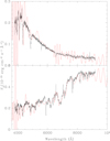 |
Fig. 9 Example spectra of WDMS binaries displaying red (top; Gaia ID 904263926328520320) and blue (bottom; Gaia ID 686844023151243904) excess clearly visible in the SDSS spectra (black) but diluted in the Gaia spectra (red). |
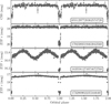 |
Fig. 10 CRTS and ZTF phase-folded photometry for 4 of the 67 eclipsing systems in the sample. Two orbits are shown for clarity and the respective Gaia DR3 source IDs are displayed in the bottom right of each panel. |
5 Eclipsing systems
Given that a significant number of the systems in our sample are likely to have evolved through a common-envelope phase and, consequently, have short orbital periods, we should expect a fraction to have an orbital inclination that would indicate they are eclipsing. We cross-matched the 1312 WDMS binaries in the sample with the catalogue of eclipsing WDMS binaries from the Zwicky Transient Facility (ZTF; Dekany et al. 2020) by van Roestel et al., in prep.) returning 63 matches. Altogther, 20 of these are in the sub-sample of 435 systems with good VOSA two-body fits and they therefore have estimates of their parameters. Follow-up observations of these objects will hence allow us to determine the masses and radii that can be directly compared to those estimated here. In order to identify any southern eclipsing systems, we also checked photometry from the Catalina Realtime Transient Survey DR3 (CRTS; Drake et al. 2009), following the method outlined in Parsons et al. (2013) and only targeted objects outside of the ZTF footprint. We found four eclipsing systems, although we note that CRTS does not go as deep as ZTF. We obtained the orbital periods of the eclipsing systems we have identified in both surveys by applying standard Lomb-Scargle periodograms to the light curves; then using a box least -squares periodogram to refine the periods (see some examples in Figure 10). These results are given in Table 2.
Estimates for the fraction of eclipsing post-commonenvelope binaries (PCEBs) containing a WD and a low-mass MS companion typically lie around 12-18% (Parsons et al. 2013; Santos-García et al. 2025), but the exact fraction depends on the orbital period distribution as well as the mass (and, therefore, the radius) distributions of the two stars. The number of eclipsing systems within the sample can therefore provide a lower limit on the fraction of PCEBs in our catalogue (a lower limit because not all eclipsing systems will be detected). Of the 1312 systems in the full sample, 920 of these are accessible to the ZTF survey (declination > −31 degrees), of which 63 are found to be eclipsing. Assuming that eclipsing systems account for 12-18% of PCEBs, this suggests that at least ≃38-57% of the full sample are PCEBs. Performing the same analysis for the sub-sample of 435 systems with reliable fits to the Gaia spectroscopy (Section 3 and Figure 5), we find that at least ≃31-46% of these are PCEBs.
The estimated PCEB fraction among WDMS in our sample seems to be higher than expected. Numerical simulations indicate that PCEBs account for approximately 25-30% of the total WDMS population (Willems & Kolb 2004; Toonen & Nelemans 2013), including the Gaia 100 pc sample (Santos-García et al. 2025). Observational studies reveal similar PCEB fractions (Schreiber et al. 2010; Nebot Gómez-Morán et al. 2011; Rebassa-Mansergas et al. 2011). It is therefore plausible that some observational biases affect the Gaia WDMS sample, which favour the detection of eclipsing systems. For example, as mentioned in Section 3, a magnitude-limited WDMS sample favours the detection of low-mass WDs, since these are more luminous for a fixed effective temperature (Rebassa-Mansergas et al. 2011). Moreover, the wider the orbital separations, the more likely it is for Gaia to resolve the two components, which would imply a bias towards shorter period systems. In the same way, wide binaries are more likely to be associated with larger values of RUWE and/or an excess factor, making them objects that could be excluded by our quality cuts. It is also worth noting that our estimated PCEB fractions assume that the cuts performed in magnitude-colour space do not impact the likelihood of a PCEBs to eclipse. For a more accurate estimate of the PCEB fraction, population synthesis techniques (e.g. Santos-García et al. 2025) will be required.
6 Summary and conclusions
Over the last two decades, it has been shown that WDMS binaries are of great use in improving our understanding of a wide range of topics in astronomy. These approaches rely on the existence of statistically large and well-defined samples that allow for the characterisation of the biases affecting the observed populations. In this sense, in this work we have built a sample of 1312 WDMS binaries by mining the spectroscopic content of the data release 3 of Gaia.
The catalogue is expected to be ≃50 per cent complete. The missing targets are predominantly expected to be objects with large values of RUWE and/or large excess noise parameters, as well as objects with mild blue or red excess in their optical spectra, which are features that are diluted in the low-resolution Gaia spectra. The identification of such WDMS stars is expected to improve thanks to the use of artificial intelligence algorithms applied to the Gaia spectra (Echeverry et al. 2022; Li et al. 2025; Pérez-Couto et al. 2025), although they fail to detect a non-negligible fraction of WDMS binaries and often misclassify irregular spectra. Moreover, the completeness dramatically drops to ≃5 per cent (lower limit) if we consider that not all WDMS binaries in Gaia have available spectra. However, despite these issues, our catalogue is very well characterised in terms of implemented photometric and astrometric cuts and observational biases and hence can be directly compared to synthetic samples that reproduce the WDMS binary population in the Galaxy to constrain, for example, binary star evolution (Santos-García et al. 2025). In addition, the study of exotic objects in the sample, such as the 67 identified eclipsing systems (which represent 5% of the total sample), allows us to place tighter constraints on the massradius relation of both WDs and low-mass MS stars (Parsons et al. 2017, 2018).
We found the catalogue to be dominated by binaries where the MS companion contributes more in the optical spectral energy distribution. Because of this, the stellar parameters that we derived for most of the WDs in these objects should be considered with caution. Future follow-up spectroscopic observations at higher resolution are therefore desired for better characterization of the WDs. Hence, these sources are excellent supplementary targets for the forthcoming White Dwarf Binary Survey (Toloza et al. 2023) implemented in the overall 4-metre Multi-Object Spectroscopic Telescope (4MOST) survey (de Jong et al. 2022).
Data availability
Table 2 is available at the CDS via anonymous ftp to cdsarc.cds.unistra.fr (130.79.128.5) or via https://cdsarc.cds.unistra.fr/viz-bin/cat/J/A+A/699/A153
Acknowledgements
We thank Enrique García-Zamora for helping with the construction of the confusion matrices. We thank the anonymous referee for the comments and suggestions on the manuscript. This work was partially supported by the Spanish MINECO grant PID2023-148661NB-I00 and by the AGAUR/Generalitat de Catalunya grant SGR-386/2021. This work was partially supported by the Spanish Virtual Observatory (https://svo.cab.inta-csic.es project funded by MCIN/AEI/10.13039/501100011033/) through grant PID2023-146210NB-I00. RMO is funded by INTA through grant PRE-OBSERVATORIO. RR acknowledges support from Grant RYC2021-030837-I, funded by MCIN/AEI/ 10.13039/501100011033 and by “European Union NextGeneration EU/PRTR”. MC acknowledges grant RYC2021-032721-I, funded by MCIN/AEI/10.13039/501100011033 and by the European Union NextGenerationEU/PRTR. This work presents results from the European Space Agency (ESA) space mission Gaia. Gaia data are being processed by the Gaia Data Processing and Analysis Consortium (DPAC). Funding for the DPAC is provided by national institutions, in particular the institutions participating in the Gaia MultiLateral Agreement (MLA). The Gaia mission website is https://www.cosmos.esa.int/gaia. The Gaia archive website is https://archives.esac.esa.int/gaia. This job has made use of the Python package GaiaXPy, developed and maintained by members of the Gaia Data Processing and Analysis Consortium (DPAC), and in particular, Coordination Unit 5 (CU5), and the Data Processing Centre located at the Institute of Astronomy, Cambridge, UK (DPCI).
References
- Allard, F., Homeier, D., Freytag, B., Schaffenberger, W., & Rajpurohit, A. S. 2013, Mem. Soc. Astron. Ital. Suppl., 24, 128 [Google Scholar]
- Althaus, L. G., Miller Bertolami, M. M., & Córsico, A. H. 2013, A&A, 557, A19 [NASA ADS] [CrossRef] [EDP Sciences] [Google Scholar]
- Anguiano, B., Majewski, S. R., Stassun, K. G., et al. 2022, AJ, 164, 126 [CrossRef] [Google Scholar]
- Arseneau, S., Chandra, V., Hwang, H.-C., et al. 2024, ApJ, 963, 17 [NASA ADS] [Google Scholar]
- Bailer-Jones, C. A. L. 2023, AJ, 166, 269 [NASA ADS] [CrossRef] [Google Scholar]
- Barrientos, M., & Chanamé, J. 2021, ApJ, 923, 181 [NASA ADS] [CrossRef] [Google Scholar]
- Bayo, A., Rodrigo, C., Barrado Y Navascués, D., et al. 2008, A&A, 492, 277 [NASA ADS] [CrossRef] [EDP Sciences] [Google Scholar]
- Belokurov, V., Penoyre, Z., Oh, S., et al. 2020, MNRAS, 496, 1922 [Google Scholar]
- Benitez, N., Dupke, R., Moles, M., et al. 2014, arXiv e-prints [arXiv:1403.5237] [Google Scholar]
- Bianchi, L., Shiao, B., & Thilker, D. 2017, ApJS, 230, 24 [Google Scholar]
- Brown, A. J., Parsons, S. G., van Roestel, J., et al. 2023, MNRAS, 521, 1880 [NASA ADS] [CrossRef] [Google Scholar]
- Bruch, A., & Diaz, M. P. 1998, AJ, 116, 908 [Google Scholar]
- Camacho, J., Torres, S., García-Berro, E., et al. 2014, A&A, 566, A86 [NASA ADS] [CrossRef] [EDP Sciences] [Google Scholar]
- Camisassa, M. E., Althaus, L. G., Córsico, A. H., et al. 2016, ApJ, 823, 158 [CrossRef] [Google Scholar]
- Camisassa, M. E., Althaus, L. G., Córsico, A. H., et al. 2019, A&A, 625, A87 [NASA ADS] [CrossRef] [EDP Sciences] [Google Scholar]
- Chen, X., Wang, S., Deng, L., et al. 2020, ApJS, 249, 18 [NASA ADS] [CrossRef] [Google Scholar]
- Chiti, F., van Saders, J. L., Heintz, T. M., et al. 2024, ApJ, 977, 15 [NASA ADS] [CrossRef] [Google Scholar]
- Cojocaru, R., Rebassa-Mansergas, A., Torres, S., & García-Berro, E. 2017, MNRAS, 470, 1442 [NASA ADS] [CrossRef] [Google Scholar]
- Cui, X.-Q., Zhao, Y.-H., Chu, Y.-Q., et al. 2012, Res. Astron. Astrophys., 12, 1197 [Google Scholar]
- Davis, P. J., Kolb, U., & Willems, B. 2010, MNRAS, 403, 179 [Google Scholar]
- de Jong, R. S., Bellido-Tirado, O., Brynnel, J. G., et al. 2022, SPIE Conf. Ser., 12184, 1218414 [NASA ADS] [Google Scholar]
- Dekany, R., Smith, R. M., Riddle, R., et al. 2020, PASP, 132, 038001 [NASA ADS] [CrossRef] [Google Scholar]
- Drake, A. J., Djorgovski, S. G., Mahabal, A., et al. 2009, ApJ, 696, 870 [Google Scholar]
- Echeverry, D., Torres, S., Rebassa-Mansergas, A., & Ferrer-Burjachs, A. 2022, A&A, 667, A144 [NASA ADS] [CrossRef] [EDP Sciences] [Google Scholar]
- Eisenstein, D. J., Weinberg, D. H., Agol, E., et al. 2011, AJ, 142, 72 [Google Scholar]
- Evans, D. W., Riello, M., De Angeli, F., et al. 2018, A&A, 616, A4 [NASA ADS] [CrossRef] [EDP Sciences] [Google Scholar]
- Farihi, J., Hoard, D. W., & Wachter, S. 2010, ApJS, 190, 275 [NASA ADS] [CrossRef] [Google Scholar]
- Gaia Collaboration (Brown, A. G. A., et al.) 2018, A&A, 616, A1 [NASA ADS] [CrossRef] [EDP Sciences] [Google Scholar]
- Gaia Collaboration (Montegriffo, P., et al.) 2023, A&A, 674, A33 [CrossRef] [EDP Sciences] [Google Scholar]
- Garbutt, J. A., Parsons, S. G., Toloza, O., et al. 2024, MNRAS, 529, 4840 [NASA ADS] [CrossRef] [Google Scholar]
- Gentile Fusillo, N. P., Tremblay, P.-E., Gänsicke, B. T., et al. 2019, MNRAS, 482, 4570 [Google Scholar]
- Grondin, S. M., Drout, M. R., Nordhaus, J., et al. 2024, ApJ, 976, 102 [Google Scholar]
- Hallakoun, N., Shahaf, S., Mazeh, T., Toonen, S., & Ben-Ami, S. 2024, ApJ, 970, L11 [Google Scholar]
- Koester, D. 2010, Mem. Soc. Astron. Italiana, 81, 921 [NASA ADS] [Google Scholar]
- Kosakowski, A., Kilic, M., Brown, W. R., Bergeron, P., & Kupfer, T. 2022, MNRAS, 516, 720 [NASA ADS] [CrossRef] [Google Scholar]
- Lallement, R., Vergely, J. L., Valette, B., et al. 2014, A&A, 561, A91 [NASA ADS] [CrossRef] [EDP Sciences] [Google Scholar]
- Li, J., Ting, Y.-S., Rix, H.-W., et al. 2025, arXiv e-prints [arXiv:2501.14494] [Google Scholar]
- Lindegren, L., Lammers, U., Hobbs, D., et al. 2012, A&A, 538, A78 [NASA ADS] [CrossRef] [EDP Sciences] [Google Scholar]
- Mamajek, E. E., & Hillenbrand, L. A. 2008, ApJ, 687, 1264 [Google Scholar]
- Marín-Franch, A., Chueca, S., Moles, M., et al. 2012, SPIE Conf. Ser., 8450, 84503S [Google Scholar]
- Marsh, T. R., Gänsicke, B. T., Hümmerich, S., et al. 2016, Nature, 537, 374 [NASA ADS] [CrossRef] [Google Scholar]
- Mowlavi, N., Holl, B., Lecoeur-Taïbi, I., et al. 2023, A&A, 674, A16 [NASA ADS] [CrossRef] [EDP Sciences] [Google Scholar]
- Nayak, P. K., Ganguly, A., & Chatterjee, S. 2024, MNRAS, 527, 6100 [Google Scholar]
- Nebot Gómez-Morán, A., Schwope, A. D., Schreiber, M. R., et al. 2009, A&A, 495, 561 [NASA ADS] [CrossRef] [EDP Sciences] [Google Scholar]
- Nebot Gómez-Morán, A., Gänsicke, B. T., Schreiber, M. R., et al. 2011, A&A, 536, A43 [NASA ADS] [CrossRef] [EDP Sciences] [Google Scholar]
- O’Donoghue, D., Koen, C., Kilkenny, D., et al. 2003, MNRAS, 345, 506 [CrossRef] [Google Scholar]
- Paczynski, B. 1976, in Structure and Evolution of Close Binary Systems, eds. P. Eggleton, S. Mitton, & J. Whelan, IAU Symposium, 73, 75 [Google Scholar]
- Parsons, S. G., Gänsicke, B. T., Marsh, T. R., et al. 2013, MNRAS, 429, 256 [Google Scholar]
- Parsons, S. G., Agurto-Gangas, C., Gänsicke, B. T., et al. 2015, MNRAS, 449, 2194 [NASA ADS] [CrossRef] [Google Scholar]
- Parsons, S. G., Rebassa-Mansergas, A., Schreiber, M. R., et al. 2016, MNRAS, 463, 2125 [Google Scholar]
- Parsons, S. G., Gänsicke, B. T., Marsh, T. R., et al. 2017, MNRAS, 470, 4473 [Google Scholar]
- Parsons, S. G., Gänsicke, B. T., Marsh, T. R., et al. 2018, MNRAS, 481, 1083 [Google Scholar]
- Parsons, S. G., Brown, A. J., Casewell, S. L., et al. 2025, MNRAS, 537, 2112 [Google Scholar]
- Penoyre, Z., Belokurov, V., & Evans, N. W. 2022, MNRAS, 513, 5270 [Google Scholar]
- Pérez-Couto, X., Manteiga, M., & Villaver, E. 2025, arXiv e-prints [arXiv:2503.04672] [Google Scholar]
- Priyatikanto, R., Knigge, C., Scaringi, S., Brink, J., & Buckley, D. A. H. 2022, MNRAS, 516, 1183 [Google Scholar]
- Pyrzas, S., Gänsicke, B. T., Marsh, T. R., et al. 2009, MNRAS, 394, 978 [NASA ADS] [CrossRef] [Google Scholar]
- Pyrzas, S., Gänsicke, B. T., Brady, S., et al. 2012, MNRAS, 419, 817 [NASA ADS] [CrossRef] [Google Scholar]
- Raddi, R., Torres, S., Rebassa-Mansergas, A., et al. 2022, A&A, 658, A22 [NASA ADS] [CrossRef] [EDP Sciences] [Google Scholar]
- Raddi, R., Rebassa-Mansergas, A., Torres, S., et al. 2025, A&A, 695, A131 [NASA ADS] [CrossRef] [EDP Sciences] [Google Scholar]
- Rebassa-Mansergas, A., Gänsicke, B. T., Rodríguez-Gil, P., Schreiber, M. R., & Koester, D. 2007, MNRAS, 382, 1377 [CrossRef] [Google Scholar]
- Rebassa-Mansergas, A., Gänsicke, B. T., Schreiber, M. R., et al. 2008, MNRAS, 390, 1635 [NASA ADS] [Google Scholar]
- Rebassa-Mansergas, A., Gänsicke, B. T., Schreiber, M. R., Koester, D., & Rodríguez-Gil, P. 2010, MNRAS, 402, 620 [Google Scholar]
- Rebassa-Mansergas, A., Nebot Gómez-Morán, A., Schreiber, M. R., Girven, J., & Gänsicke, B. T. 2011, MNRAS, 413, 1121 [NASA ADS] [CrossRef] [Google Scholar]
- Rebassa-Mansergas, A., Nebot Gómez-Morán, A., Schreiber, M. R., et al. 2012, MNRAS, 419, 806 [NASA ADS] [CrossRef] [Google Scholar]
- Rebassa-Mansergas, A., Schreiber, M. R., & Gänsicke, B. T. 2013, MNRAS, 429, 3570 [NASA ADS] [CrossRef] [Google Scholar]
- Rebassa-Mansergas, A., Anguiano, B., García-Berro, E., et al. 2016a, MNRAS, 463, 1137 [NASA ADS] [CrossRef] [Google Scholar]
- Rebassa-Mansergas, A., Ren, J. J., Parsons, S. G., et al. 2016b, MNRAS, 458, 3808 [NASA ADS] [CrossRef] [Google Scholar]
- Rebassa-Mansergas, A., Parsons, S. G., García-Berro, E., et al. 2017, MNRAS, 466, 1575 [NASA ADS] [CrossRef] [Google Scholar]
- Rebassa-Mansergas, A., Parsons, S. G., Dhillon, V. S., et al. 2019, Nat. Astron., 3, 553 [Google Scholar]
- Rebassa-Mansergas, A., Maldonado, J., Raddi, R., et al. 2021a, MNRAS, 505, 3165 [NASA ADS] [CrossRef] [Google Scholar]
- Rebassa-Mansergas, A., Solano, E., Jiménez-Esteban, F. M., et al. 2021b, MNRAS, 506, 5201 [NASA ADS] [CrossRef] [Google Scholar]
- Rebassa-Mansergas, A., Maldonado, J., Raddi, R., et al. 2023, MNRAS, 526, 4787 [NASA ADS] [CrossRef] [Google Scholar]
- Ren, J. J., Rebassa-Mansergas, A., Parsons, S. G., et al. 2018, MNRAS, 477, 4641 [NASA ADS] [CrossRef] [Google Scholar]
- Ren, J. J., Raddi, R., Rebassa-Mansergas, A., et al. 2020, ApJ, 905, 38 [NASA ADS] [CrossRef] [Google Scholar]
- Riello, M., De Angeli, F., Evans, D. W., et al. 2021, A&A, 649, A3 [NASA ADS] [CrossRef] [EDP Sciences] [Google Scholar]
- Rybizki, J., Green, G. M., Rix, H.-W., et al. 2022, MNRAS, 510, 2597 [NASA ADS] [CrossRef] [Google Scholar]
- Santos-García, A., Torres, S., Rebassa-Mansergas, A., & Brown, A. J. 2025, A&A, 695, A161 [NASA ADS] [CrossRef] [EDP Sciences] [Google Scholar]
- Schreiber, M. R., Gänsicke, B. T., Rebassa-Mansergas, A., et al. 2010, A&A, 513, L7 [NASA ADS] [CrossRef] [EDP Sciences] [Google Scholar]
- Schreiber, M. R., Belloni, D., Gänsicke, B. T., Parsons, S. G., & Zorotovic, M. 2021, Nat. Astron., 5, 648 [NASA ADS] [CrossRef] [Google Scholar]
- Shahaf, S., Hallakoun, N., Mazeh, T., et al. 2024, MNRAS, 529, 3729 [NASA ADS] [CrossRef] [Google Scholar]
- Sidharth, A. V., Shridharan, B., Mathew, B., et al. 2024, A&A, 690, A68 [NASA ADS] [CrossRef] [EDP Sciences] [Google Scholar]
- Skrutskie, M. F., Cutri, R. M., Stiening, R., et al. 2006, AJ, 131, 1163 [NASA ADS] [CrossRef] [Google Scholar]
- Toloza, O., Rebassa-Mansergas, A., Raddi, R., et al. 2023, The Messenger, 190, 4 [NASA ADS] [Google Scholar]
- Toonen, S., & Nelemans, G. 2013, A&A, 557, A87 [NASA ADS] [CrossRef] [EDP Sciences] [Google Scholar]
- Torres, S., Canals, P., Jiménez-Esteban, F. M., Rebassa-Mansergas, A., & Solano, E. 2022, MNRAS, 511, 5462 [NASA ADS] [CrossRef] [Google Scholar]
- Webbink, R. F. 2008, in Astrophysics and Space Science Library, eds. E. F. Milone, D. A. Leahy, & D. W. Hobill, Astrophysics and Space Science Library, 352, 233 [Google Scholar]
- Willems, B., & Kolb, U. 2004, A&A, 419, 1057 [NASA ADS] [CrossRef] [EDP Sciences] [Google Scholar]
- Wright, N. J., Newton, E. R., Williams, P. K. G., Drake, J. J., & Yadav, R. K. 2018, MNRAS, 479, 2351 [Google Scholar]
- Yamaguchi, N., El-Badry, K., Rees, N. R., et al. 2024, PASP, 136, 084202 [Google Scholar]
- Zhao, J. K., Oswalt, T. D., Willson, L. A., Wang, Q., & Zhao, G. 2012, ApJ, 746, 144 [Google Scholar]
- Zorotovic, M., Schreiber, M. R., Gänsicke, B. T., & Nebot Gómez-Morán, A. 2010, A&A, 520, A86 [NASA ADS] [CrossRef] [EDP Sciences] [Google Scholar]
- Zorotovic, M., Schreiber, M. R., Parsons, S. G., et al. 2016, MNRAS, 457, 3867 [Google Scholar]
See http://svo2.cab.inta-csic.es/theory/vosa/helpw4.php?otype=star&what=intro for a description on how the bolometric flux is derived.
Note: the decomposition/fitting routine of the SDSS WDMS binary spectra yields secondary spectral types rather than effective temperatures (Rebassa-Mansergas et al. 2010). We converted the spectral types into temperatures using the relation of Rebassa-Mansergas et al. (2007), which is virtually identical to the updated tables of Mamajek & Hillenbrand (2008).
All Tables
All Figures
|
Fig. 1 Results of our criteria imposed on the Gaia date release 3 data base to select WDMS binaries (see details in Section 2). Top-left: 126 787 sources within the WDMS binary region defined by the black solid lines (Rebassa-Mansergas et al. 2021b) shown in blue with the available spectra and satisfying parallax and flux relative errors above 10%. The gray dots illustrate the expected location of single WD and MS stars. Top-right: same as top-left, after applying our excess factor and astrometry (RUWE; astrometric_excess_noise and astrometric_excess_noise_sig) cuts, which leaves 62 386 objects. Bottom-left: same after excluding single stars using VOSA, leaving 13 905 candidates. Bottom right: final catalogue of 1312 WDMS binaries after visual inspection of the Gaia spectra. |
| In the text | |
|
Fig. 2 Example spectra of a WDMS binary (top, Gaia ID 1057463111970047488. Note: in this work, we use the DR3 IDs), a cataclysmic variable (middle top: Gaia ID 3703726255561754880), a hot WD (middle bottom: Gaia ID1060659289192635904) and a low-mass low-metallicity subdwarf as revealed by the broad absorption feature at ~7000 Å (bottom: Gaia ID 1048217078174314496) arising from the visual inspection of the Gaia spectra. |
| In the text | |
|
Fig. 3 Example images illustrating WDMS candidates (red squares) for being contaminated by the presence of nearby sources. Left panel: POSS/DSS blue image of Gaia ID 2055951194776633600. Right panel: Pan-STARSS g-band image of Gaia ID 2776554794743195648. |
| In the text | |
|
Fig. 4 Example of two-body VOSA fits. The top panel shows a typical MS-dominated WDMS binary in our sample. The combination of models (purple for the secondary star and cyan for the WD) seem to fit relatively well the observed data (red dots). However, the effective temperature of the WD is too low. Clearly, such a low-luminosity WD would not be seen against a 3000 K secondary M star. The middle panel illustrates an example of a bad fit, especially in the ultraviolet range. The bottom panel shows what we consider a good fit, where the models match the observed data at all wavelengths. |
| In the text | |
|
Fig. 5 Distribution of WD effective temperatures, surface gravities, masses, and secondary star effective temperatures derived from 435 WDMS binaries with reliable VOSA two-body fits, shown from top to bottom. |
| In the text | |
|
Fig. 6 Comparison among the WD effective temperatures (bottom) and surface gravities (middle) as well as MS star effective temperatures (top) for 54 WDMS binaries with VOSA reliable two-body fits and spectroscopic parameters derived from SDSS spectra. The black dashed lines indicate the one to one relation, whilst the red dashed lines are linear fits to the data. Note: in the top panel, values above 3700 K in the horizontal axis were not considered. |
| In the text | |
|
Fig. 7 Confusion matrices representing the level of agreement between our catalogue and other samples: Rebassa-Mansergas et al. (2021b) at the top-left, Nayak et al. (2024) at the top-right, Li et al. (2025) at the bottom-left, and the SDSS WDMS sample at the bottom-right. The values within the matrices indicate the number of targets falling in each category and the percentages respect to the total number of objects in each row. In particular, the top-left cells in each matrix indicate the number and fraction of common objects, whilst the diagonal cells indicate the number of objects (and fractions) missed (or not included) by the corresponding works. |
| In the text | |
|
Fig. 8 Example spectra of WDMS binaries in the list of Li et al. (2025) that we do not consider as such. Gaia source IDs are 767397543537053312 (top) and 5952567592693723904 (bottom). |
| In the text | |
|
Fig. 9 Example spectra of WDMS binaries displaying red (top; Gaia ID 904263926328520320) and blue (bottom; Gaia ID 686844023151243904) excess clearly visible in the SDSS spectra (black) but diluted in the Gaia spectra (red). |
| In the text | |
|
Fig. 10 CRTS and ZTF phase-folded photometry for 4 of the 67 eclipsing systems in the sample. Two orbits are shown for clarity and the respective Gaia DR3 source IDs are displayed in the bottom right of each panel. |
| In the text | |
Current usage metrics show cumulative count of Article Views (full-text article views including HTML views, PDF and ePub downloads, according to the available data) and Abstracts Views on Vision4Press platform.
Data correspond to usage on the plateform after 2015. The current usage metrics is available 48-96 hours after online publication and is updated daily on week days.
Initial download of the metrics may take a while.