| Issue |
A&A
Volume 684, April 2024
|
|
|---|---|---|
| Article Number | A103 | |
| Number of page(s) | 11 | |
| Section | Catalogs and data | |
| DOI | https://doi.org/10.1051/0004-6361/202347617 | |
| Published online | 09 April 2024 | |
The search for DA double white dwarf binary candidates from SDSS DR14
1
Shandong Provincial Key Laboratory of Optical Astronomy and Solar-Terrestrial Environment, School of Space Science and Physics, Shandong University at Weihai,
Weihai
264209,
PR China
e-mail: This email address is being protected from spambots. You need JavaScript enabled to view it.
2
CAS Key Laboratory of Optical Astronomy, National Astronomical Observatories, Chinese Academy of Sciences,
Beijing
100101,
PR China
3
Department of Scientific Research, Beijing Planetarium,
Xizhimenwai Street,
Beijing
100044,
PR China
4
Yunnan Observatories, Chinese Academy of Sciences,
Kunming,
650011,
PR China
5
Key Laboratory of Stars and Interstellar Medium, Xiangtan University,
Xiangtan
411105,
PR China
6
School of Astronomy and Space Science, University of Chinese Academy of Sciences,
Beijing
100049,
PR China
Received:
1
August
2023
Accepted:
31
January
2024
Abstract
Aims. Double white dwarf (DWD) binaries are one of the channels through which type Ia supernovae explosions occur. With the release of more and more sky survey data, the search for additional DWDs has become a possibility. We utilized the spectroscopic data from SDSS DR14 to search for DWD binaries based on variations in radial velocities (RVs).
Methods. We obtained a sample of 4089 DA white dwarfs (WDs) with two or more spectra from SDSS DR14, and their RVs were derived using the cross-correlation function. Using the chi-squared (χ2) distribution of RVs as a base, we calculated the corresponding logarithmic probabilities (log p) for different degrees of freedom.
Results. We selected the targets with log p < −3.0 and obtained 65 highly credible DWD candidates, of which 56 were newly discovered. We compared the distributions of the Teff, log g, and mass of the DWD candidates and found that the mass distribution of DWDs has two peaks. The primary peak, located at 0.45 M⊙, is lower than the peak of the total WD sample, while the secondary peak, located at 0.60 M⊙, is similar to the peak of the total sample. Finally, we crossmatched our sample with Zwicky Transient Facility (ZTF) photometry data and identified two targets with clear periodic variability. Based on the shape of their light curve, we think both could be white dwarf main-sequence binary stars
Key words: techniques: radial velocities / binaries: general / white dwarfs
© The Authors 2024
 Open Access article, published by EDP Sciences, under the terms of the Creative Commons Attribution License (https://creativecommons.org/licenses/by/4.0), which permits unrestricted use, distribution, and reproduction in any medium, provided the original work is properly cited.
This article is published in open access under the Subscribe to Open model. This email address is being protected from spambots. You need JavaScript enabled to view it. to support open access publication.
1 Introduction
White dwarfs (WDs) are the final evolutionary outcome of main-sequence (MS) stars with masses ranging from 0.07 M⊙ to 10 M⊙ (Doherty et al. 2014). It is estimated that approximately 97% of stars will eventually evolve into WDs (Fontaine et al. 2001; Heger et al. 2003; Woosley & Heger 2015; Lauffer et al. 2018). So, WDs play a crucial role in the overall stellar population of the Galaxy and serve as precise indicators of the formation and evolution of the Milky Way (Winget et al. 1987; Torres et al. 2005; Tremblay et al. 2014). From spectro-scopic, photometric, or asteroseismic analyses, the fundamental properties of WDs, including mass, cooling age, atmospheric composition, and internal composition, can be determined (Bergeron et al. 1992, 2001, 2011; Koester et al. 2009; Tremblay et al. 2013; Romero et al. 2017; Giammichele et al. 2018). Based on their spectral characteristics, WDs are mainly classified into two types: DA and DB. Because of the relatively short timescales of gravitational settling, the atmospheric composition of WDs tends to be simple. In the case of DA WDs, sinking timescales can be as short as a few days, whereas for non-DA WDs, sinking timescales typically range from 0.01 to 1 million years (Koester & Wilken 2006; Koester 2009; Wyatt et al. 2014). Approximately 80% of WDs exhibit only hydrogen lines in their spectra, which corresponds to the spectral class DA. When the atmospheric temperature of WDs is high enough to excite helium atoms, the spectra of most of the remaining WDs are dominated by helium lines, which corresponds to the spectral class DB. A very detailed classification of WD types was proposed by McCook & Sion (2016).
As has been widely recognized, the multiplicity frequency (MF) of MS stars exhibits a pronounced and consistent correlation with their stellar mass. For Sun-like stars, the MF is approximately 50%. More massive stars exhibit significantly higher MFs (greater than 60% or even higher), while M dwarfs and very low-mass stars (VLMs) have a lower MF (approximately 30%; Duchêne & Kraus 2013; Moe & Di Stefano 2017). According to the Roche lobe, binary stars can be classified into three types. Detached binary stars: in this type of binary stars, the stars are relatively far apart from each other and do not significantly affect each other’s shape or evolution. Each star is within its own Roche lobe, the region around the star where material is gravitationally bound, and there is no material flowing in or out. Semi-detached binary stars: in this type of binary stars, one of the star fills up the equipotential surface of its Roche lobe and through the first Lagrangian point (L1) transfers mass to the second component. Contact binary stars: in this type of binary stars, both stars’ Roche lobes have material flowing out, causing their surfaces to come into contact with each other, forming a binary system with a shared envelope of material. Contact binary stars often exhibit complex phenomena of mass transfer and stellar evolution as material is continuously exchanged between the two stars.
Type Ia supernovae (SNe Ia) have played a pivotal role in the investigation of cosmic evolution, particularly as standardizable candles that have contributed to the discovery of the accelerated expansion of the Universe (Riess et al. 1998; Schmidt et al. 1998; Perlmutter et al. 1999). The origin of SNe Ia is commonly attributed to the thermonuclear explosions of WDs in binary systems (Hoyle & Fowler 1960). Nevertheless, there is currently a lack of consensus regarding the fundamental characteristics of SNe Ia and their explosion mechanisms, both in the theoretical and observational domains (e.g., Wang & Han 2012; Hillebrandt et al. 2013; Maoz et al. 2014; Maeda & Terada 2016; Livio & Mazzali 2018; Soker 2019; Ruiter 2020; Liu et al. 2023, for reviews). There are generally two scenarios for SNe Ia: one is the single-degenerate (SD) scenario, and the other is the double-degenerate (DD) Scenario.
In the SD scenario, a WD accretes material from a non-degenerate companion star until its mass approaches the Chan-drasekhar mass (about 1.4 M⊙), triggering a thermonuclear explosion (Schatzman 1963; Wheeler & Hansen 1971; Whelan & Iben 1973; Nomoto 1982b,a; Nomoto et al. 1984). In the original DD scenario, a binary system consists of two carbon-oxygen (CO) WDs that come into contact due to the emission of gravitational waves. They merge through tidal interaction to form a single entity, potentially causing a SN Ia explosion if their combined mass surpasses the Chandrasekhar-mass limit (Iben & Tutukov 1984; Webbink 1984).
Numerous simulations over recent decades have explored the merger of two WDs, offering insights into SN Ia mechanisms beyond the original DD scenario. Notably, these studies reveal alternative pathways for SN Ia explosions. For example, the “violent merger model.” During the intense merger phase of two CO WDs, a carbon detonation can be directly initiated as the debris from the secondary WD interacts with the primary WD, ultimately leading to the occurrence of a SN Ia explosion (Pakmor et al. 2010, 2012; Sato et al. 2015). If the secondary WD in a DD binary system is a pure He WD, it can initiate an initial He detonation by accumulating a He shell atop the primary CO WD through stable mass transfer, and thus eventually trigger a C-core detonation at the core, leading to a successful SN Ia explosion. This represents the sub-Chandrasekhar-mass double-detonation scenario (Fink et al. 2007, 2010; Moll & Woosley 2013; Gronow et al. 2020, 2021; Boos et al. 2021; Liu et al. 2023). Additionally, unstable mass transfer can introduce He into the surface layers of the primary CO WD, whether the secondary WD is a He WD or a hybrid HeCO WD, potentially resulting in a SN Ia during the coalescence itself through the double-detonation mechanism (Guillochon et al. 2010; Roy et al. 2022; Liu et al. 2023). Presently, the DD scenario and its variants are the more popular scenarios.
Currently, searching for WD binaries based on radial velocity (RV) variations is a relatively reliable method. The initial systematic attempts to search detached close double white dwarfs (DWDs) were conducted during the 1980s through the method of RV variation, yielding limited results (Robinson & Shafter 1987; Bragaglia et al. 1990; Foss et al. 1991). With the continuous release of data from surveys such as LAMOST (Zhao et al. 2012, 2006, 2013; Guo et al. 2022), SDSS (York et al. 2000; Kepler et al. 2019), and Gaia (e.g., Gentile Fusillo et al. 2021; Gaia Collaboration 2021), an increasing number of WDs are being discovered. This provides more favorable conditions for us to search for WD binaries and several groups have used these data to identify or characterize WD binaries.
For example, from the SDSS spectroscopic catalog, based on variations in RV, Badenes et al. (2009) found a single-lined spec-troscopic WD binary in a circular orbit; Mullally et al. (2009) discovered two of the shortest-period non-interacting binary WD stars; Badenes & Maoz (2012) employed the catalog to estimate the rate at which WD binaries merge within the Milky Way Galaxy; Breedt et al. (2017) used the large sample to preselect candidates and test the DD model for SNe Ia; and Chandra et al. (2021) discovered a double-lined WD binary. Over the last decade, the Extremely Low Mass (ELM) survey conducted by Brown et al. (2010), which was tailored to focus on He-core WDs with masses below 0.3 M⊙ using a color-based selection, has successfully detected up to 98 new DWDs, as was reported in the study by Brown et al. (2020). Utilizing LAMOST spectra and the Gaia DR2 data, Wang et al. (2022) found a total of 136 ELM WD candidates and 12 previously identified objects from the ELM Survey. Gianninas et al. (2015) searched for binary stars composed of a WD and a MS (WDMS) companion based on RV variations. Rebassa-Mansergas et al. (2021) also conducted a search for unresolved WDMS within a 100 pc range using data provided by Gaia EDR3. A total of 112 objects were selected based on their positions in the Hertzsprung-Russell diagram (HRD), of which 97 were newly identified.
The combination of photometric survey data can lead to a more effective search for DWDs. Steinfadt et al. (2010) discovered a DWD using photometric survey data in 2010, while the Kepler K2 (Howell et al. 2014) mission discovered a new WD binary among the 1 000 WDs (Hallakoun et al. 2016; van Sluijs & Van Eylen 2018). The Zwicky Transient Facility (ZTF; Bellm et al. 2019; Graham et al. 2019; Masci et al. 2019), which commenced operations in 2018, has already identified approximately ten newly discovered ultra-compact DWDs (Burdge et al. 2019, 2020; Coughlin et al. 2020; Keller et al. 2022; van Roestel et al. 2021). Ren et al. (2023) has compiled a catalog of candidate close double white dwarf (CWDB) systems with short periods, using data from the Gaia EDR3 catalog and ZTF photometry data. In the foreseeable future, extensive all-sky surveys like Gaia (Gaia Collaboration 2016, 2018, 2021) and the Vera Rubin Observatory (LSST Science Collaboration 2009) hold the potential to reveal hundreds and even thousands of new DWD systems, respectively (Korol et al. 2017).
In this article, we have selected DWD candidates based on spectral data provided by SDSS DR14, using variation in the RV to identify binary candidates. The paper is organized as follows. In Sect. 2, we introduce the sample of DA WD data and the method of RV measurement, as well as binary candidate identification based on the variation of RVs. Section 3 compares the Teff, log g, and mass of the DA DWD binary candidates with the total sample. In Sect. 4, we crossmatch the ZTF data to obtain the period of optical variability for the DA WD binary candidates. The conclusions of the study are presented in Sect. 5.
2 Data and radial velocity measurement
2.1 Data
The SDSS spectroscopic data contains the spectra of numerous WDs. By analyzing the spectra of all stars in the SDSS DR14, (Kepler et al. 2019) report 20 088 spectrally confirmed WDs and classify them based on their spectral characteristics. Since the number of DA WDs with high-quality spectra and multiple observations in DR16 (Kepler et al. 2021) is almost same as that in DR14, in the current study we used the data sample provided in DR14. In the end, we obtained 4089 DA WDs with multiple spectroscopic observations (approximately 14 000 pieces of spectral data).
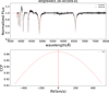 |
Fig. 1 Spectrum normalization and CCF curve. Top: the red solid line indicates the normalized template spectrum, and the black solid line is the normalized observed spectrum. Bottom: the red solid line shows the CCF curve, and the red dashed line shows the RV value. |
2.2 Radial velocity measurement
Due to the broadening of absorption lines in WDs, calculating the RV based on the line center shift may lead to significant errors. Here, we used the cross-correlation method (CCF; Tonry & Davis 1979) to measure the RV of WDs. The traditional advantage of the CCF is its ability to be accelerated using fast Fourier transformation (FFT), but the drawback is that the resulting CCF has sparse sampling. Zhang et al. (2020, 2021) have made improvements to address this issue, and in this paper we adopted the method for computing the CCF proposed by Zhang et al. (2020, 2021). The template spectra of DA WDs are the theoretical spectra generated by Koester (2010). First, both the template and observed spectra of the WDs underwent normalization using the toolkit developed by Chandra et al. (2020), which was specifically designed for processing WD spectra. Chandra et al. (2020) initially applied a composite model, which includes a Voigt profile combined with a linear function of wavelength, to a region encompassing each Balmer line from Hα to H8. Subsequently, they derived the continuum-normalized spectrum for each line by dividing the region around it by the linear component of the composite fit. Finally, the RVs were calculated using the CCF method.
The range of variation for the RVs was set from −500 km s−1 to 500 km s−1 with an interval of 1 km s−1. The velocity value corresponding to the peak of the CCF curve represents the RV of the respective spectrum. Figure 1 shows an example of RV estimation. We employed Monte Carlo (MC) simulations to assess the uncertainties associated with our RV measurements. The fundamental approach involved generating a set of simulated spectra, each based on an observed spectrum, and subsequently deriving their RV values from the CCF. The RV uncertainty was then adopted by the standard deviation in these RV values. To perform this analysis, we created 100 simulated spectra for each observed spectrum. In these simulated spectra, the flux at each wavelength point was drawn from a Gaussian distribution, with the mean and variance of the Gaussian distribution determined by the flux and flux error of the corresponding observed spectrum. Figure 2 displays the normalized spectra. The gray lines represent 100 simulated spectra, while the red line represents the observed spectrum. Figure A.1 displays the corresponding CCF curves for the 100 simulated spectra and one observed spectrum. The black line represents the CCF curve of 100 simulated spectra, while the red line represents the CCF curve of the observed spectrum. It is evident that the simulated spectra we generated are evenly distributed around the observed spectrum. However, due to the added error in the simulated spectra, their signal-to-noise ratio (S/N) is inferior to that of the observed spectrum, resulting in lower CCF curves for the simulated spectra compared to the observed spectrum.
2.3 Selection criteria
As is depicted in Fig. A.2, the relationship between the errors of RVs and the spectral S/N reveals a clear trend: as the S/N increases, the RV errors decrease. To assess the reliability of our error, we employed the same method as Maoz & Hallakoun (2017). Since the majority of the sample consists of single WDs, the distributions of observed RV differences between two epochs of observations of the same WDs should follow a Gaussian distribution, centered around zero and with a σ corresponding to the RV error estimate, except for the minority of DWDs with real RV changes between epochs. We have compared the mean RV error estimate from every pair of epochs for the same WD to the actual RV difference between those epochs, scaled down by  . Figure 3 demonstrates an alignment with the anticipated expectation, depicting the distributions of observed RV epoch differences within specific ranges of the calculated RV errors.
We used the same method for the variability as was used by Maxted et al. (2000), Napiwotzki et al. (2020), Geier et al. (2022). We computed the weighted mean RV of each star by taking into account the inverse variance of all measured epochs. Assuming this mean velocity to be constant, we then calculated the χ2 statistic. By comparing this calculated value with the χ2-distribution for the appropriate degrees of freedom, we determined the probability (P) of obtaining the observed χ2 value or a higher value from random fluctuations around a constant velocity. A detection of RV variability is considered significant if the false detection P is less than 0.1% (log p < −3.0). Figure A.3 shows the histogram of the distribution of log p. From the spectral information of candidates, they exhibit single-line systems, but there is a possibility that some candidates have a dim M dwarf or brown dwarf as companions. Because some WDMS binary systems are predominantly dominated by the WD in the optical wavelength, they appear as a single WD in the spectrum. To mitigate these influences, we performed a crossmatch with the WDMS catalog provided by Rebassa-Mansergas et al. (2010, 2021) and removed one confirmed WDMS target. Additionally, based on the catalog provided by Girven et al. (2011), we also removed one target known to have a photometric infrared excess that potentially had a faint dwarf star as a companion. Next, we queried these candidates on SIMBAD (Wenger et al. 2000) and discovered that nine targets have been confirmed as WD binary systems (the corresponding markings were made in Table A.1). In the end, we obtained a total of 66 WD binary candidates, of which 57 were newly identified candidates.
Table 1 shows the RVs of all DA WDs (the top five WDs; the full table can be found in the supplementary material). Table A.1 shows the log p for the DA DWD binary candidates.
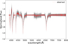 |
Fig. 2 Normalized spectra of the generated 100 simulated spectra (gray line) and the normalized spectra of the observed spectra (red line). |
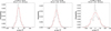 |
Fig. 3 Distributions of RV differences between two epochs of the same WDs, scaled down by |

RVs of all DA WDs.
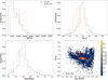 |
Fig. 4 Histograms of Teff, log g, and mass (solid black line representing all the WDs; dashed red line representing the WD binary candidates) and the distribution of log Teff and log g (red dots representing WD binary candidates; 2D histogram representing all the WDs). |
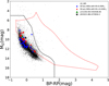 |
Fig. 5 Distribution of the WD binary candidates and the sample of general WDs on HRD (BP-RP vs. absolute G). WD binary candidates less than 0.45 M⊙ are represented by red dots, WD binary candidates greater than 0.45 M⊙ by blue dots, and the total sample of DA WDs by black dots. DWD J151343.50+443436.40 is represented by a green triangle and WDMS J003221.88+073934 by a black pentagon. The solid black line shows a color-cut and absolute magnitude selection scheme for searching for WDs using Gaia data proposed by Gentile Fusillo et al. (2019). The dashed red lines show the selection scheme for searching for WDMS candidates based on Gaia EDR3 data by Rebassa-Mansergas et al. (2021). |
3 Parameters of the DA WD binary candidates
3.1 Teff, log g, and masses of WD binary candidates and single WDs
Kepler et al. (2019) calculated the Teff, log g, and masses of WD samples based on the spectrum. We compared these three physical parameters between DWD binary candidates and single WDs. Figure 4 displays the distributions of Teff, log g, and mass. In the histogram, the solid black line represents all WDs, while the dashed red line represents the 66 DWD binary candidates. In the scatter plot, black dots represent the distributions of Teff and log g for all the WDs, while red dots represent the distributions of Teff and log g for the DWD binary candidates.
The WD binary candidates exhibit bimodal distributions in both Teff and log g. This leads to the presence of two peaks in the mass distribution, one at 0.45 M⊙ (lower than the peak of the overall sample) and one at 0.58 M⊙ (similar to the peak of the overall sample). The occurrence of such a mass distribution is within the expected range. Due to the inability of single stars to evolve into such low-mass WDs within the Hubble time, there is a higher proportion of low-mass WDs in binary systems (Brown et al. 2016; Rebassa-Mansergas et al. 2011; Breedt et al. 2017; Napiwotzki et al. 2020). We divided the overall sample into low-mass WDs and high-mass WDs using a mass threshold of 0.45. Then, we plotted their cumulative distribution functions (CDFs) of log P. As is shown in Fig. A.4, the red line represents the CDF of low-mass WDs, while the dashed black line represents the CDF of high-mass WDs. Our selection criterion is log p < −3.0. As is clearly shown in Fig. A.4, it is evident that the proportion of low-mass WDs (6%) is higher than that of high-mass (1%) WDs. The different mass distribution of our DWD binary candidates may be due to different evolution.
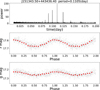 |
Fig. 6 Power spectrum light curve and phase folding diagram of J151343.50+443436.40. The middle and bottom panels show the ZTF r-band and g-band folded light curves, respectively. The gray dots represent the folded light curves of all data. The red dots show the averaged light curve with data points averaged every 0.05 phase bins. |
3.2 Gaia Hertzsprung-Russell diagram
We divided the WD binary candidates into two parts with mass equal to 0.45 M⊙ and drew them on the HRD, as is shown in Fig. 5, which displays the distribution of the BP-RP color index with respect to the G magnitude on the HRD. The black dots on the diagram represent the distribution of all samples of WDs, while the red dots represent the distribution of DWD binary candidates with masses below 0.45 M⊙. The blue dots represent the DWD binary candidates with masses above 0.45 M⊙. The solid black line represents the boundary for selecting WDs based on the HRD (Gentile Fusillo et al. 2019), while the dashed red line represents the range of boundaries for selecting WD+MS binary systems, as is suggested by Rebassa-Mansergas et al. (2021) based on the stellar evolution model. However, we examined the WD binary candidates in the dashed red line region, and their spectra do not exhibit the spectral features of MS stars. This was expected, since this region serves only as an initial selection of WD+MS candidates and could also include double WDs.
4 Zwicky Transient Facility photometry
The ZTF is a 48-in. (P48) Schmidt telescope used at the Palomar Observatory for time-domain surveys. With a field of view of 47 deg2, it can scan the entire visible northern sky (with a declination greater than −28°) at a rate of approximately 3750 square degrees per hour (Dekany et al. 2020; Graham et al. 2019; Masci et al. 2019). ZTF can achieve a 5σ S/N limit of about 20.8 mag in the g band, 20.6 mag in the r band, and 20.2 mag in the i band with 30-s exposures.
We crossmatched the obtained binary star candidates with ZTF DR161 and used a Lomb–Scargle (LS) periodogram analysis to calculate the periods of the corresponding light curves. In the end, we identified two targets with clear periodic variability: J151343.50+443436.40 and J003221.88+073934.30. J003221.88+073934.30 was certified by Rebassa-Mansergas et al. (2010) as being a WD+MS binary system. Table 2 shows the information for these two targets. Based on the light curves, we believe that these two stars may both be WD+MS binary systems and that the variability may be caused by a reflection effect rather than ellipsoidal distortion. Faigler & Mazeh (2011) conducted research to estimate the modulation amplitude expected from ellipsoidal effects and reflection. The observed modulation amplitude is more consistent with a reflection effect, and larger than expected from ellipsoidal effects alone.
The variability may be caused by the ellipsoidal distortion of the other MS sub-star. Since WDs are relatively small and dense, they are not easily distorted. The amplitude of the distortion depends on the degree of ellipsoidal distortion, with larger amplitudes corresponding to greater distortion. Additionally, the magnetic field of the WD also has some influence. In Fig. 5, the green triangle and the black pentagon, respectively, indicate their locations on the HRD. Figures 6 and 7 show the power spectra and light curves of two binary candidates with apparent periods. Figure A.5 shows the spectra of these two systems.
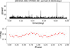 |
Fig. 7 Power spectrum and phase folding diagram of WDJ003221.88+073934.30. This is consistent with Fig. 6. |
Parameters of the two systems with the measured orbital period.
5 Conclusions
In this work, we aimed to find DWD binary candidates based on RV variations. We used DA WD data from SDSS DR14 provided by Kepler et al. (2019) to filter out about 4000 targets with multiple spectroscopic observations. Their RVs were calculated by the CCF method, and the targets with log P < −3.0 were selected as DWD binary candidates according to the screening criteria of Maxted et al. (2000), Napiwotzki et al. (2020), Geier et al. (2022). Finally, 65 highly plausible DWD binary candidates were obtained, and 56 were newly identified candidates.
We compared the physical parameters of the DWD binary candidates and the total sample of WDs, and found that DWD binary candidates have two peaks in the mass distribution: one is 0.45 M⊙, which is lower than the peak mass of the total sample of WDs, and the other is 0.58 M⊙, which is consistent with the total sample of WDs. We further divided the DWD sample into two parts using 0.45 M⊙ as the limit and found a higher proportion of low-mass DWD binary candidates, in agreement with the findings of the ESO VLT data of Napiwotzki et al. (2020). The proportion of low-mass DWD binary candidates among the DA WDs is 6.0%, while the proportion of high-mass DWD candidates is 1.0%. We plotted the two parts of the DWD sample divided according to the mass on the HRD.
Finally, we crossed the candidate data with ZTF data and used LS to find the light curve period. We looked for two discovered targets with significant periods and calculated their periods. Based on the light curves, we believe that they are both more likely to be WD+MS binary systems.
Acknowledgements
We thank National Natural Science Foundation of China 11988101, 12273055, 11890694, 11973048, 11927804, 12203006 and the Innovation Project of Beijing Academy of Science and Technology (11000023T000002062763-23CB059). We also acknowledge the support from the 2m Chinese Space Station Telescope project: CMS-CSST-2021-A10. Thanks to Zhang Bin for the discussion and suggestions for this work.
Appendix A Additional material
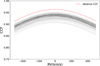 |
Fig. A.1 CCF curves of 100 simulated spectra (black line) and CCF curves of observed spectra (red line). |
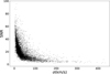 |
Fig. A.2 S/N of spectra vs. RV uncertainties of the WDs. |
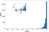 |
Fig. A.3 Histogram displaying the number of targets at different log p values, with the bar chart in the top left corner showing the distribution of targets within the log p < −3.0 range. |
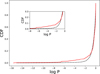 |
Fig. A.4 Cumulative distribution functions of log P. The solid red line represents low-mass WDs; the black dashed line represents high-mass WDs. |
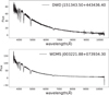 |
Fig. A.5 Spectra of the two systems with period: J151343.50+443436.40 and J003221.88+073934.30. |
log p for the DA DWD binary candidates
References
- Badenes, C., & Maoz, D. 2012, ApJ, 749, L11 [NASA ADS] [CrossRef] [Google Scholar]
- Badenes, C., Mullally, F., Thompson, S. E., & Lupton, R. H. 2009, ApJ, 707, 971 [NASA ADS] [CrossRef] [Google Scholar]
- Bellm, E. C., Kulkarni, S. R., Graham, M. J., et al. 2019, PASP, 131, 018002 [Google Scholar]
- Bergeron, P., Saffer, R. A., & Liebert, J. 1992, ApJ, 394, 228 [NASA ADS] [CrossRef] [Google Scholar]
- Bergeron, P., Leggett, S. K., & Ruiz, M. T. 2001, ApJS, 133, 413 [Google Scholar]
- Bergeron, P., Wesemael, F., Dufour, P., et al. 2011, ApJ, 737, 28 [NASA ADS] [CrossRef] [Google Scholar]
- Boos, S. J., Townsley, D. M., Shen, K. J., Caldwell, S., & Miles, B. J. 2021, ApJ, 919, 126 [NASA ADS] [CrossRef] [Google Scholar]
- Bragaglia, A., Greggio, L., Renzini, A., & D’Odorico, S. 1990, ApJ, 365, L13 [NASA ADS] [CrossRef] [Google Scholar]
- Breedt, E., Steeghs, D., Marsh, T. R., et al. 2017, MNRAS, 468, 2910 [NASA ADS] [CrossRef] [Google Scholar]
- Brown, W. R., Kilic, M., Allende Prieto, C., & Kenyon, S. J. 2010, ApJ, 723, 1072 [Google Scholar]
- Brown, J. M., Kilic, M., Brown, W. R., & Kenyon, S. J. 2011, ApJ, 730, 67 [NASA ADS] [CrossRef] [Google Scholar]
- Brown, W. R., Gianninas, A., Kilic, M., Kenyon, S. J., & Allende Prieto, C. 2016, ApJ, 818, 155 [Google Scholar]
- Brown, W. R., Kilic, M., Kosakowski, A., et al. 2020, ApJ, 889, 49 [Google Scholar]
- Burdge, K. B., Coughlin, M. W., Fuller, J., et al. 2019, Nature, 571, 528 [Google Scholar]
- Burdge, K. B., Prince, T. A., Fuller, J., et al. 2020, ApJ, 905, 32 [Google Scholar]
- Chandra, V., Hwang, H.-C., Zakamska, N. L., & Budavári, T. 2020, MNRAS, 497, 2688 [NASA ADS] [CrossRef] [Google Scholar]
- Chandra, V., Hwang, H.-C., Zakamska, N. L., et al. 2021, ApJ, 921, 160 [NASA ADS] [CrossRef] [Google Scholar]
- Coughlin, M. W., Burdge, K., Phinney, E. S., et al. 2020, MNRAS, 494, L91 [NASA ADS] [CrossRef] [Google Scholar]
- Dekany, R., Smith, R. M., Riddle, R., et al. 2020, PASP, 132, 038001 [NASA ADS] [CrossRef] [Google Scholar]
- Doherty, C. L., Gil-Pons, P., Siess, L., Lattanzio, J. C., & Lau, H. H. B. 2014, MNRAS, 446, 2599 [Google Scholar]
- Duchêne, G., & Kraus, A. 2013, ARA&A, 51, 269 [Google Scholar]
- Faigler, S., & Mazeh, T. 2011, MNRAS, 415, 3921 [Google Scholar]
- Fink, M., Hillebrandt, W., & Röpke, F. K. 2007, A&A, 476, 1133 [NASA ADS] [CrossRef] [EDP Sciences] [Google Scholar]
- Fink, M., Röpke, F. K., Hillebrandt, W., et al. 2010, A&A, 514, A53 [NASA ADS] [CrossRef] [EDP Sciences] [Google Scholar]
- Fontaine, G., Brassard, P., & Bergeron, P. 2001, PASP, 113, 409 [NASA ADS] [CrossRef] [Google Scholar]
- Foss, D., Wade, R. A., & Green, R. F. 1991, ApJ, 374, 281 [CrossRef] [Google Scholar]
- Gaia Collaboration (Prusti, T., et al.) 2016, A&A, 595, A1 [NASA ADS] [CrossRef] [EDP Sciences] [Google Scholar]
- Gaia Collaboration (Brown, A. G. A., et al.) 2018, A&A, 616, A1 [NASA ADS] [CrossRef] [EDP Sciences] [Google Scholar]
- Gaia Collaboration (Brown, A. G. A., et al.) 2021, A&A, 649, A1 [NASA ADS] [CrossRef] [EDP Sciences] [Google Scholar]
- Geier, S., Dorsch, M., Pelisoli, I., et al. 2022, A&A, 661, A113 [NASA ADS] [CrossRef] [EDP Sciences] [Google Scholar]
- Gentile Fusillo, N. P., Tremblay, P.-E., Gänsicke, B. T., et al. 2019, MNRAS, 482, 4570 [Google Scholar]
- Gentile Fusillo, N. P., Tremblay, P. E., Cukanovaite, E., et al. 2021, MNRAS, 508, 3877 [NASA ADS] [CrossRef] [Google Scholar]
- Giammichele, N., Charpinet, S., Fontaine, G., et al. 2018, Nature, 554, 73 [NASA ADS] [CrossRef] [Google Scholar]
- Gianninas, A., Kilic, M., Brown, W. R., Canton, P., & Kenyon, S. J. 2015, ApJ, 812, 167 [Google Scholar]
- Girven, J., Gänsicke, B. T., Steeghs, D., & Koester, D. 2011, MNRAS, 417, 1210 [Google Scholar]
- Graham, M. J., Kulkarni, S. R., Bellm, E. C., et al. 2019, PASP, 131, 078001 [Google Scholar]
- Gronow, S., Collins, C., Ohlmann, S. T., et al. 2020, A&A, 635, A169 [NASA ADS] [CrossRef] [EDP Sciences] [Google Scholar]
- Gronow, S., Collins, C. E., Sim, S. A., & Röpke, F. K. 2021, A&A, 649, A155 [NASA ADS] [CrossRef] [EDP Sciences] [Google Scholar]
- Guillochon, J., Dan, M., Ramirez-Ruiz, E., & Rosswog, S. 2010, ApJ, 709, L64 [Google Scholar]
- Guo, J., Zhao, J., Zhang, H., et al. 2022, MNRAS, 509, 2674 [NASA ADS] [Google Scholar]
- Hallakoun, N., Maoz, D., Kilic, M., et al. 2016, MNRAS, 458, 845 [NASA ADS] [CrossRef] [Google Scholar]
- Heger, A., Fryer, C. L., Woosley, S. E., Langer, N., & Hartmann, D. H. 2003, ApJ, 591, 288 [CrossRef] [Google Scholar]
- Hillebrandt, W., Kromer, M., Röpke, F. K., & Ruiter, A. J. 2013, Front. Phys., 8, 116 [Google Scholar]
- Howell, S. B., Sobeck, C., Haas, M., et al. 2014, PASP, 126, 398 [Google Scholar]
- Hoyle, F., & Fowler, W. A. 1960, ApJ, 132, 565 [NASA ADS] [CrossRef] [Google Scholar]
- Iben, I. J., & Tutukov, A. V. 1984, ApJ, 284, 719 [NASA ADS] [CrossRef] [Google Scholar]
- Keller, P. M., Breedt, E., Hodgkin, S., et al. 2022, MNRAS, 509, 4171 [Google Scholar]
- Kepler, S. O., Pelisoli, I., Koester, D., et al. 2019, MNRAS, 486, 2169 [NASA ADS] [Google Scholar]
- Kepler, S. O., Koester, D., Pelisoli, I., Romero, A. D., & Ourique, G. 2021, MNRAS, 507, 4646 [NASA ADS] [CrossRef] [Google Scholar]
- Koester, D. 2009, A&A, 498, 517 [NASA ADS] [CrossRef] [EDP Sciences] [Google Scholar]
- Koester, D. 2010, Mem. Soc. Astron. Italiana, 81, 921 [NASA ADS] [Google Scholar]
- Koester, D., & Wilken, D. 2006, A&A, 453, 1051 [NASA ADS] [CrossRef] [EDP Sciences] [Google Scholar]
- Koester, D., Voss, B., Napiwotzki, R., et al. 2009, A&A, 505, 441 [NASA ADS] [CrossRef] [EDP Sciences] [Google Scholar]
- Korol, V., Rossi, E. M., Groot, P. J., et al. 2017, MNRAS, 470, 1894 [NASA ADS] [CrossRef] [Google Scholar]
- Lauffer, G. R., Romero, A. D., & Kepler, S. O. 2018, MNRAS, 480, 1547 [NASA ADS] [CrossRef] [Google Scholar]
- Liu, Z.-W., Röpke, F. K., & Han, Z. 2023, Res. Astron. Astrophys., 23, 082001 [CrossRef] [Google Scholar]
- Livio, M., & Mazzali, P. 2018, Phys. Rep., 736, 1 [Google Scholar]
- LSST Science Collaboration (Abell, P. A., et al.) 2009, arXiv e-prints [arXiv:0912.0201] [Google Scholar]
- Maeda, K., & Terada, Y. 2016, Int. J. Mod. Phys. D, 25, 1630024 [NASA ADS] [CrossRef] [Google Scholar]
- Maoz, D., & Hallakoun, N. 2017, MNRAS, 467, 1414 [Google Scholar]
- Maoz, D., Mannucci, F., & Nelemans, G. 2014, ARA&A, 52, 107 [Google Scholar]
- Masci, F. J., Laher, R. R., Rusholme, B., et al. 2019, PASP, 131, 018003 [Google Scholar]
- Maxted, P. F. L., Marsh, T. R., & Moran, C. K. J. 2000, MNRAS, 319, 305 [Google Scholar]
- McCook, G. P., & Sion, E. M. 2016, VizieR Online Data Catalog: 1/2035 [Google Scholar]
- Moe, M., & Di Stefano, R. 2017, ApJS, 230, 15 [Google Scholar]
- Moll, R., & Woosley, S. E. 2013, ApJ, 774, 137 [NASA ADS] [CrossRef] [Google Scholar]
- Mullally, F., Badenes, C., Thompson, S. E., & Lupton, R. 2009, ApJ, 707, L51 [NASA ADS] [CrossRef] [Google Scholar]
- Napiwotzki, R., Karl, C. A., Lisker, T., et al. 2020, A&A, 638, A131 [NASA ADS] [CrossRef] [EDP Sciences] [Google Scholar]
- Nomoto, K. 1982a, ApJ, 253, 798 [Google Scholar]
- Nomoto, K. 1982b, ApJ, 257, 780 [Google Scholar]
- Nomoto, K., Thielemann, F. K., & Yokoi, K. 1984, ApJ, 286, 644 [Google Scholar]
- Pakmor, R., Kromer, M., Röpke, F. K., et al. 2010, Nature, 463, 61 [Google Scholar]
- Pakmor, R., Kromer, M., Taubenberger, S., et al. 2012, ApJ, 747, L10 [NASA ADS] [CrossRef] [Google Scholar]
- Perlmutter, S., Aldering, G., Goldhaber, G., et al. 1999, ApJ, 517, 565 [Google Scholar]
- Rebassa-Mansergas, A., Gänsicke, B. T., Schreiber, M. R., Koester, D., & Rodríguez-Gil, P. 2010, MNRAS, 402, 620 [Google Scholar]
- Rebassa-Mansergas, A., Nebot Gómez-Morán, A., Schreiber, M. R., Girven, J., & Gänsicke, B. T. 2011, MNRAS, 413, 1121 [NASA ADS] [CrossRef] [Google Scholar]
- Rebassa-Mansergas, A., Solano, E., Jiménez-Esteban, F. M., et al. 2021, MNRAS, 506, 5201 [NASA ADS] [CrossRef] [Google Scholar]
- Ren, L., Li, C., Ma, B., et al. 2023, ApJS, 264, 39 [NASA ADS] [CrossRef] [Google Scholar]
- Riess, A. G., Filippenko, A. V., Challis, P., et al. 1998, AJ, 116, 1009 [Google Scholar]
- Robinson, E. L., & Shafter, A. W. 1987, ApJ, 322, 296 [CrossRef] [Google Scholar]
- Romero, A. D., Córsico, A. H., Castanheira, B. G., et al. 2017, ApJ, 851, 60 [NASA ADS] [CrossRef] [Google Scholar]
- Roy, N. C., Tiwari, V., Bobrick, A., et al. 2022, ApJ, 932, L24 [NASA ADS] [CrossRef] [Google Scholar]
- Ruiter, A. J. 2020, in White Dwarfs as Probes of Fundamental Physics: Tracers of Planetary, Stellar and Galactic Evolution, eds. M. A. Barstow, S. J. Kleinman, J. L. Provencal, & L. Ferrario, 357, 1 [NASA ADS] [Google Scholar]
- Sato, Y., Nakasato, N., Tanikawa, A., et al. 2015, ApJ, 807, 105 [NASA ADS] [CrossRef] [Google Scholar]
- Schatzman, E. 1963, in Star Evolution, ed. L. Gratton, 389 [Google Scholar]
- Schmidt, B. P., Suntzeff, N. B., Phillips, M. M., et al. 1998, ApJ, 507, 46 [NASA ADS] [CrossRef] [Google Scholar]
- Soker, N. 2019, New A Rev., 87, 101535 [NASA ADS] [CrossRef] [Google Scholar]
- Steinfadt, J. D. R., Kaplan, D. L., Shporer, A., Bildsten, L., & Howell, S. B. 2010, ApJ, 716, L146 [NASA ADS] [CrossRef] [Google Scholar]
- Tonry, J., & Davis, M. 1979, AJ, 84, 1511 [Google Scholar]
- Torres, S., García-Berro, E., Isern, J., & Figueras, F. 2005, MNRAS, 360, 1381 [CrossRef] [Google Scholar]
- Tremblay, P. E., Bergeron, P., & Gianninas, A. 2011, ApJ, 730, 128 [Google Scholar]
- Tremblay, P. E., Ludwig, H. G., Steffen, M., & Freytag, B. 2013, A&A, 559, A104 [NASA ADS] [CrossRef] [EDP Sciences] [Google Scholar]
- Tremblay, P. E., Kalirai, J. S., Soderblom, D. R., Cignoni, M., & Cummings, J. 2014, ApJ, 791, 92 [NASA ADS] [CrossRef] [Google Scholar]
- van Roestel, J., Creter, L., Kupfer, T., et al. 2021, AJ, 162, 113 [NASA ADS] [CrossRef] [Google Scholar]
- van Sluijs, L., & Van Eylen, V. 2018, MNRAS, 474, 4603 [NASA ADS] [CrossRef] [Google Scholar]
- Wang, B., & Han, Z. 2012, New A Rev., 56, 122 [CrossRef] [Google Scholar]
- Wang, K., Németh, P., Luo, Y., et al. 2022, ApJ, 936, 5 [CrossRef] [Google Scholar]
- Webbink, R. F. 1984, ApJ, 277, 355 [NASA ADS] [CrossRef] [Google Scholar]
- Wenger, M., Ochsenbein, F., Egret, D., et al. 2000, A&AS, 143, 9 [NASA ADS] [CrossRef] [EDP Sciences] [Google Scholar]
- Wheeler, J. C., & Hansen, C. J. 1971, Ap&SS, 11, 373 [Google Scholar]
- Whelan, J., & Iben, Icko, J. 1973, ApJ, 186, 1007 [CrossRef] [Google Scholar]
- Winget, D. E., Hansen, C. J., Liebert, J., et al. 1987, ApJ, 315, L77 [CrossRef] [Google Scholar]
- Woosley, S. E., & Heger, A. 2015, ApJ, 810, 34 [NASA ADS] [CrossRef] [Google Scholar]
- Wyatt, M. C., Farihi, J., Pringle, J. E., & Bonsor, A. 2014, MNRAS, 439, 3371 [CrossRef] [Google Scholar]
- York, D. G., Adelman, J., Anderson, John E., J., et al. 2000, AJ, 120, 1579 [NASA ADS] [CrossRef] [Google Scholar]
- Zhang, B., Liu, C., & Deng, L.-C. 2020, ApJS, 246, 9 [NASA ADS] [CrossRef] [Google Scholar]
- Zhang, B., Li, J., Yang, F., et al. 2021, ApJS, 256, 14 [NASA ADS] [CrossRef] [Google Scholar]
- Zhao, G., Chen, Y.-Q., Shi, J.-R., et al. 2006, Chinese J. Astron. Astrophys., 6, 265 [NASA ADS] [CrossRef] [Google Scholar]
- Zhao, G., Zhao, Y.-H., Chu, Y.-Q., Jing, Y.-P., & Deng, L.-C. 2012, Res. Astron. Astrophys., 12, 723 [NASA ADS] [CrossRef] [Google Scholar]
- Zhao, J. K., Luo, A. L., Oswalt, T. D., & Zhao, G. 2013, AJ, 145, 169 [NASA ADS] [CrossRef] [Google Scholar]
All Tables
All Figures
|
Fig. 1 Spectrum normalization and CCF curve. Top: the red solid line indicates the normalized template spectrum, and the black solid line is the normalized observed spectrum. Bottom: the red solid line shows the CCF curve, and the red dashed line shows the RV value. |
| In the text | |
|
Fig. 2 Normalized spectra of the generated 100 simulated spectra (gray line) and the normalized spectra of the observed spectra (red line). |
| In the text | |
|
Fig. 3 Distributions of RV differences between two epochs of the same WDs, scaled down by |
| In the text | |
|
Fig. 4 Histograms of Teff, log g, and mass (solid black line representing all the WDs; dashed red line representing the WD binary candidates) and the distribution of log Teff and log g (red dots representing WD binary candidates; 2D histogram representing all the WDs). |
| In the text | |
|
Fig. 5 Distribution of the WD binary candidates and the sample of general WDs on HRD (BP-RP vs. absolute G). WD binary candidates less than 0.45 M⊙ are represented by red dots, WD binary candidates greater than 0.45 M⊙ by blue dots, and the total sample of DA WDs by black dots. DWD J151343.50+443436.40 is represented by a green triangle and WDMS J003221.88+073934 by a black pentagon. The solid black line shows a color-cut and absolute magnitude selection scheme for searching for WDs using Gaia data proposed by Gentile Fusillo et al. (2019). The dashed red lines show the selection scheme for searching for WDMS candidates based on Gaia EDR3 data by Rebassa-Mansergas et al. (2021). |
| In the text | |
|
Fig. 6 Power spectrum light curve and phase folding diagram of J151343.50+443436.40. The middle and bottom panels show the ZTF r-band and g-band folded light curves, respectively. The gray dots represent the folded light curves of all data. The red dots show the averaged light curve with data points averaged every 0.05 phase bins. |
| In the text | |
|
Fig. 7 Power spectrum and phase folding diagram of WDJ003221.88+073934.30. This is consistent with Fig. 6. |
| In the text | |
|
Fig. A.1 CCF curves of 100 simulated spectra (black line) and CCF curves of observed spectra (red line). |
| In the text | |
|
Fig. A.2 S/N of spectra vs. RV uncertainties of the WDs. |
| In the text | |
|
Fig. A.3 Histogram displaying the number of targets at different log p values, with the bar chart in the top left corner showing the distribution of targets within the log p < −3.0 range. |
| In the text | |
|
Fig. A.4 Cumulative distribution functions of log P. The solid red line represents low-mass WDs; the black dashed line represents high-mass WDs. |
| In the text | |
|
Fig. A.5 Spectra of the two systems with period: J151343.50+443436.40 and J003221.88+073934.30. |
| In the text | |
Current usage metrics show cumulative count of Article Views (full-text article views including HTML views, PDF and ePub downloads, according to the available data) and Abstracts Views on Vision4Press platform.
Data correspond to usage on the plateform after 2015. The current usage metrics is available 48-96 hours after online publication and is updated daily on week days.
Initial download of the metrics may take a while.