| Issue |
A&A
Volume 699, July 2025
|
|
|---|---|---|
| Article Number | A149 | |
| Number of page(s) | 12 | |
| Section | The Sun and the Heliosphere | |
| DOI | https://doi.org/10.1051/0004-6361/202554241 | |
| Published online | 03 July 2025 | |
The role of the Lorentz force in sunspot equilibrium
1
Institut für Sonnenphysik, Georges-Köhler-Allee 401A, D-79110 Freiburg, Germany
2
Institute for Solar Physics, Department of Astronomy, Stockholm University, AlbaNova University Centre, 10691 Stockholm, Sweden
3
High Altitude Observatory, NSF National Center for Atmospheric Research, 3080 Center Green Dr., Boulder 80301, USA
4
Max Planck Institute for Solar System Research, Justus-von-Liebig 3, D-37077 Göttingen, Germany
5
Instituto de Astrofísica de Canarias, Avd. Vía Láctea s/n, E-38205 La Laguna, Spain
6
Departamento de Astrofísica, Universidad de La Laguna, E-38205 La Laguna, Tenerife, Spain
⋆ Corresponding author.
Received:
24
February
2025
Accepted:
27
May
2025
Context. Sunspots survive on the solar surface for timescales ranging from days to months. This requires them to be in an equilibrium involving magnetic fields and hydrodynamic forces. Unfortunately, theoretical models of sunspot equilibrium are very simplified as they assume that spots are static and possess a self-similar and axially symmetric magnetic field. These assumptions neglect the role of small-scale variations of the magnetic field along the azimuthal direction produced by umbral dots, light bridges, penumbral filaments, and so forth.
Aims. We aim to study whether sunspot equilibrium is maintained once azimuthal fluctuations in the magnetic field, produced by the sunspot fine structure, are taken into account.
Methods. We apply the FIRTEZ Stokes inversion code to spectropolarimetric observations to infer the magnetic and thermodynamic parameters in two sunspots located at the disk center and observed with two different instruments: one observed from the ground with the 1.5-meter German GREGOR Telescope and another with the Japanese spacecraft Hinode. We compare our results with three-dimensional radiative magnetohydrodynamic simulations of a sunspot carried out with the MuRAM code.
Results. We infer clear variations in the gas pressure and density of the plasma directly related to fluctuations in the Lorentz force and associated with the filamentary structure in the penumbra. Similar results are obtained in the umbra despite its lack of an observed filamentary structure. Results from the two observed sunspots are in excellent qualitative and quantitative agreement with the numerical simulations.
Conclusions. Our results indicate that the magnetic topology of sunspots along the azimuthal direction is very close to magnetohydrostatic equilibrium, thereby helping to explain why sunspots are such long-lived structures capable of surviving on the solar surface for days or even full solar rotations.
Key words: magnetohydrodynamics (MHD) / polarization / Sun: magnetic fields / Sun: photosphere / sunspots
© The Authors 2025
 Open Access article, published by EDP Sciences, under the terms of the Creative Commons Attribution License (https://creativecommons.org/licenses/by/4.0), which permits unrestricted use, distribution, and reproduction in any medium, provided the original work is properly cited.
This article is published in open access under the Subscribe to Open model. Subscribe to A&A to support open access publication.
1. Introduction
Sunspots are the most prominent manifestation of the solar magnetic activity cycle (Solanki 2003). Their inner region, the umbra, is cool and appears dark. The umbra can feature so-called umbral dots and light bridges, which are intrusions of convective flows that disrupt the otherwise homogeneous magnetic field. The umbra is surrounded by a hotter and brighter halo, the penumbra, which features a very distinct filamentary structure. It is characterized by the presence of Evershed flow channels that are mostly concentrated along horizontal and radially aligned weak magnetic field lines, and that alternate in the azimuthal direction with a more vertical and stronger magnetic field (Lites et al. 1993; Solanki & Montavon 1993; Stanchfield et al. 1997).
In addition, sunspots harbor a myriad of highly dynamic phenomena that evolve on timescales comparable to the Alvén crossing timescales and convective timescales (i.e., minutes to hours in the upper atmosphere). Examples of such phenomena include umbral dots and penumbral grains (Sobotka & Jurčák 2009), overturning convection (Ichimoto et al. 2007a; Scharmer et al. 2011), waves (Bloomfield et al. 2007a,b; Löhner-Böttcher & Bello González 2015), and Evershed clouds (Cabrera Solana et al. 2007, 2008). In spite of this, and due to their long lifetimes, which span from days to several months, sunspots are thought to be in an equilibrium involving magnetohydrodynamic (MHD) forces (Rempel & Schlichenmaier 2011). However, theoretical descriptions of this equilibrium are very simplified. They assume, for instance, that the magnetic field is self-similar and axially symmetric (Low 1975, 1980a,b; Pizzo 1986, 1990; Jahn & Schmidt 1994; Khomenko & Collados 2008). This assumption completely ignores the large variations in the magnetic field in the azimuthal direction caused by small-scale features such as umbral dots (Ortiz et al. 2010), light bridges (Falco et al. 2016), and penumbral filaments. Here we address the long-neglected equilibrium along the azimuthal direction and conclusively demonstrate, using observations and numerical simulations, that in the photosphere both the umbra and penumbra are very close to azimuthal magnetohydrostatic (MHS) equilibrium despite the presence of strong inhomogeneities in the magnetic field. These results provide decisive observational and theoretical support for the idea that sunspots slowly evolve around an equilibrium state and are, in leading order, in MHS equilibrium, thereby helping to explain their long lifespans.
2. Observations
The observations analyzed in this work correspond to spectropolarimetric observations in several magnetically sensitive Fe I spectral lines of two sunspots located very close to the disk center. The first sunspot was observed from the ground using the GRIS instrument (Collados et al. 2012) attached to theGerman 1.5-meter GREGOR solar telescope (Schmidt et al. 2012), whereas the second sunspot was observed with the SP instrument (Lites et al. 2001; Ichimoto et al. 2007b) on board the Japanese spacecraft Hinode (Suematsu et al. 2008; Tsuneta et al. 2008; Shimizu et al. 2008; Kosugi et al. 2007).
For the first sunspot, GREGOR’s Infrared Spectrograph (GRIS) was used to record the Stokes vector Iobs(x, y, λ) = (I, Q, U, V) across a 4 nm wide wavelength region centered around 1565 nm and with a wavelength sampling of δλ ≈ 40 mÅ pixel−1. This wavelength region was therefore sampled with 1000 spectral points, out of which we selected a 7.6 Å wide region with Nλ = 190 spectral points that included two Fe I spectral lines (see Table 1). The spectral line Fe I 15652.8 Å was also recorded but it is not included in our analysis because in the umbra it appears blended with two molecular lines (Mathew et al. 2003) and the FIRTEZ inversion code employed in this work (see Section 3) cannot model them. During data acquisition, five accumulations of 30 ms each were recorded for each modulation state. This results in a total exposure time of 0.6 seconds per slit, yielding a noise level in the polarization signals of σq ≈ σu ≈ σv ≈ 10−3 in units of the quiet Sun continuum intensity.
Atomic parameters of the spectral lines analyzed in this work.
In the second sunspot, Hinode’s spectropolarimeter (SP) recorded the Stokes vector Iobs(x, y, λ) = (I, Q, U, V) across a ≈0.24 nm wide wavelength region around 630 nm and with a wavelength sampling of δλ ≈ 21.5 mÅ pixel−1. This wavelength region was sampled with a total of 112 spectral points including two Fe I spectral lines (see Table 1). In these data the total exposure time per slit position is 4.8 seconds, resulting in similar noise levels in the polarization signals to the ones in GREGOR data: σq ≈ σu ≈ σv ≈ 10−3 in units of the quiet Sun continuum intensity.
The first sunspot is NOAA AR 12049 and was observed on May 3, 2015. Different studies of the same sunspot have been presented elsewhere (Franz et al. 2016; Borrero et al. 2016). By correlating our images with simultaneous HMI/SDO full-disk continuum images, we estimate that the sunspot center was located at coordinates (x, y) = (73″, −83″) (measured from the disk center). These values correspond a to heliocentric angle of Θ = 6.5° (μ = 0.993). The image scale is δx = 0.135″ pixel−1 and δy = 0.136″ pixels−1 along the x and y axes, respectively. The scanned region contains Nx = 411 and Ny = 341 pixels along each spatial dimension, resulting in a total field of view of 55.5″ × 46.4″. The width of the spectrograph’s slit was set to 0.27″ (i.e., twice the scanning step). Details about the data calibration in terms of flat-fielding, spectral stray-light correction, fringe removal, and wavelength calibration can be found in Borrero et al. (2016).
The second sunspot is NOAA AR 10933 and was observed on January 6, 2007. This sunspot has already been analyzed in previous works (Franz & Schlichenmaier 2013). The sunspot center was located at coordinates (x, y) = (72″, −21″) (measured from the disk center). These values correspond to a heliocentric angle of Θ = 4.4° (μ = 0.997). The image scale is δx = 0.15″ pixel−1 and δy = 0.16″ pixels−1 along the x and y axes, respectively. The scanned region contains Nx = 350 and Ny = 300 pixels along each spatial dimension, resulting in a total field of view of 52.5″ × 48.0″.
3. Stokes inversion
In this work we have performed two distinct inversions of each of the datasets described in Sect. 2. The first one was a pixel-wise inversion whereby each spatial pixel on the solar surface (x, y) was treated independently. The second one was a point spread function (PSF)-coupled inversion employing the PSFs described in Sect. 4. In some aspects both work identically. Let us describe those first.
The inversion of the observed Stokes vector, Iobs(λ, x, y), was performed by using an initial atmospheric model described by the following physical parameters: temperature, T(x, y, z), magnetic field, B(x, y, z), and line-of-sight velocity, vz(x, y, z). On the XY plane we used the same number of (x, y) grid cells and spacing as the observations. In the vertical z direction the atmospheric model was discretized in 128 points with a vertical spacing of Δz = 12 km. The solution to the radiative transfer equation for polarized light from this initial model in the vertical direction yields the synthetic Stokes vector Isyn(λ, x, y), which was compared to the observed ones via a χ2 merit function. The FIRTEZ code also provides the analytical derivatives of the Stokes vector with respect to the aforementioned physical parameters.
It is at this point that the pixel-wise and PSF-coupled inversions differ. On the pixel-wise inversion, the derivatives atlocation (x, y) enter a Levenberg-Marquardt algorithm (Press et al. 1986), which combined with the singular value decomposition method (Golub & Kahan 1965) provides the perturbations in temperature, magnetic field, and so on, to be applied to the initial physical parameters so that the next solution to the polarized radiative transfer equation will yield a Isyn(λ, x, y) that is closer to the observed Iobs(λ, x, y) (i.e., χ2 minimization). The perturbations were only applied at discrete z locations called nodes, with the final z stratification being obtained via interpolation across the 128 vertical grid points. The number of nodes employed in this work is provided in Table 2. The matrices to be inverted, at a given spatial location, are squared matrices with the following number of elements: [N(T)×N(Bx)×N(By)×N(Bz)×N(vz)]2, where N(T) refers to the number of nodes allowed for the temperature, N(Bx) the number of nodes allowed in the x component of the magnetic field, and so forth. In this way the initial model at location (x, y) was iteratively perturbed until χ2 reaches a minimum, at which point we assumed that the resulting atmospheric model at that location is the correct one.
Number of nodes employed in the Stokes inversion.
In the PSF-coupled inversion, FIRTEZ closely follows the method originally developed by van Noort (2012). It proceeds in a similar fashion as in the pixel-wise inversion up until the χ2 calculation. The merit function was not obtained by comparing Iobs(λ, x, y) with Isyn(λ, x, y) but rather with  which results from the spatial convolution of Isyn(λ, x, y) with the instrumental PSF ℱ(x, y). Details about the PSFs used in this work are given in Section 4. Now, the derivatives of the Stokes vector with respect to the physical parameters are coupled horizontally, so that, a perturbation of a physical parameter at location (x′,y′) will affect the outgoing Stokes vector at (x, y). Therefore the χ2 minimization cannot be performed individually for each (x, y) pixel. Instead the minimization must be done at once considering all pixels on the observed region simultaneously. Because of this the square matrices to be inverted are now much larger than in the pixel-wise inversion. The number of elements is now [N(T)×N(Bx)×N(By)×N(Bz)×N(vz)×Nx × Ny]2. For the coupled inversion FIRTEZ does not employ the singular value decomposition method. Instead the coupled matrix is considered to be sparse and its inverse is found via the biconjugate stabilized gradient method (BiCGTAB; van der Vorst 1992).
Each of the two described inversions, pixel-wise and PSF-coupled, were first run under the assumption of vertical hydrostatic equilibrium (HE) for the gas pressure. Once this was done, the magnetic field from the hydrostatic inversion was modified so as to remove the 180° ambiguity in Bx and By (Metcalf et al. 2006) via the non-potential field calculation method (Georgoulis 2005). The resulting atmospheric model was then employed, as an initial guess of an inversion where the gas pressure was obtained under MHS equilibrium. A more detailed description on the approach followed can be found in Borrero et al. (2021).
From all inferred physical parameters by the Stokes inversion, in our study we focus mainly on the following ones: the module of the magnetic field, ∥B∥, inclination of the magnetic field with respect to the normal direction to the solar surface, γ = cos−1(Bz/∥B∥), gas pressure, Pg, density, ρ, and finally also the Lorentz force, L = (4π)−1(∇ × B)×B. Spatial derivatives of the magnetic field were determined by employing fourth-order centered finite differences over an angular array with a constant Δϕ step such that RΔϕ (R being the arc radius) was approximately equal to the grid size. We note that using second- or even sixth-order derivatives does not impact results.
4. Point spread functions
The PSF-coupled inversions (described in Section 3) were carried out with FIRTEZ employing the PSFs ℱ(x, y) shown in Figure 1 for GREGOR/GRIS data (left panel) and Hinode/SP data (middle panel). In the latter case, ℱ(x, y) corresponds to a diffraction-limited PSF for the SOT telescope on-board Hinode at 630 nm, including a 50 cm primary mirror with a 17.2 cm central obscuration caused by the secondary mirror and three 4 cm wide spiders and a 1.5 mm de-focus (Danilovic et al. 2008; Ebert et al. 2024). In the former case, GREGOR being a ground-based telescope subject to seeing effects, the PSF was modeled as the sum of two different contributions:
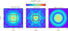 |
Fig. 1. Point spread functions employed in the data analysis. Left panel: PSF (diffraction-limited plus seeing) used in the coupled-inversion of GREGOR/GRIS data. Middle panel: PSF (diffraction-limited) used in the coupled-inversion of Hinode/SP data. For both GREGOR and Hinode data, the full PSF (±1.6 Mm) was used in the synthesis, whereas in the inversion only the square box was considered. Right panel: Ideal PSF (Airy function) used to degrade the MHD simulations. |

where ℱdiff(x, y) is the diffraction-limited PSF for a telescope operating at 1565 nm, including a 144 cm primary mirror with a 45 cm central obscuration caused by the secondary mirror and four 2.2 cm wide spiders. The second contribution, ℱseeing(x, y), is meant to approximately represent the seeing, and it was modeled as a Gaussian function with σ = 0.5″ (or ≈375 km at disk center) and carrying 43% of the energy on the detector (α = 0.43; Orozco Suárez et al. 2017). While originally we had taken a much broader Gaussian with σ = 5″ (≈3750 km at the disk center), the contribution from such a Gaussian across the employed area of ≈9 Mm2 (see Fig. 1) is essentially constant, leading to a poor convergence of the coupled inversion. A narrower Gaussian allowed the algorithm to converge much better, while still mimicking the effects of the seeing. It is worth noting that, while the actual seeing conditions change during the observations, ℱseeing is considered to be time-independent.
According to the Rayleigh criterion, if we consider only the diffraction-limited contribution to the PSFs, both GREGOR and Hinode data feature a very similar spatial resolution of about 0.3″ because, while Hinode’s primary mirror is three times smaller, it also operates at wavelengths approximately three times shorter. Even though the full PSFs in Figure 1 were employed during the synthesis and to compute the merit function χ2 between the observed and synthetic Stokes profiles (Iobs and Isyn, respectively), during the inversion (i.e., to determine the derivatives of χ2 with respect to the physical parameters) only the red squares were considered. In both cases, Hinode and GREGOR, the region enclosed by these red squares contains more than 75% of the total amount of light received by a given pixel on the detector. In the case of Hinode, the square box covers ±4 pixels along each spatial dimension around the central pixel, whereas for GREGOR the square box covers ±6 pixels. For completeness, Fig. 1 (right panel) also includes the PSF employed to degrade the MHD simulations to a spatial resolution comparable to that of GREGOR and Hinode observations (see Section 5).
5. Magnetohydrodynamic simulations
The MHD simulations employed in this work were produced with the MuRAM radiative MHD code (Vögler et al. 2005) with the specific adaptations for sunspot simulations that are described in Rempel et al. (2009a,b) and Rempel (2011, 2012). The code solves the fully compressible MHD equations using a tabulated equation of state that accounts for partial ionization in the solar atmosphere assuming equilibrium ionization (based on the OPAL package by Rogers et al. 1996). The radiation transport module computes rays in 24 directions using a short characteristics approach as described in Vögler et al. (2005). We used four-band opacities that group spectral lines according to their contribution height in the solar atmosphere.
We used a sunspot simulation run started from Rempel (2012), whereby the magnetic field at the top boundary was forced to be more horizontal with the parameter α = 2 (see Appendix B). We continued the simulation at a horizontal resolution of 32 × 32 km and with a 16 km vertical resolution while using non-gray radiative transfer with four opacity bins. The very same simulation, but using a different timestamp, was employed in Jurčák et al. (2020). The data (Pg, ρ, and B) with the original 32 × 32 km resolution was convolved with the PSF presented in Sect. 4 (see also rightmost panel in Fig. 1). This PSF consists of an Airy function where the first minimum is located at a distance of 232 km from the peak. This is equivalent to about 0.3″ at the disk center, and therefore very similar to the ideal (i.e., diffraction-limited) spatial resolution in GREGOR and Hinode data (see Section 4). We note that, after the application of this PSF, the data from the MHD simulation were further binned from 32 × 32 down to 128 × 128 km so as to also have a comparable spatial sampling as in the observed data. From there, γ, ∥B∥, and L were calculated. The Lorentz force in the MHD simulations was also calculated employing fourth-order centered finite differences to determine the spatial derivatives of the magnetic field (see Section 3). A summary of the physical properties in the simulations is displayed in Figure 2 (third column). Further details about the initial and boundary conditions are given in Appendix B.
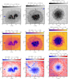 |
Fig. 2. Summary of analyzed data and inversion results. Top row: Continuum intensity normalized to the average quiet Sun intensity, Ic/Ic, qs. Middle row: Temperature, T. Bottom row: Inclination of the magnetic field, γ, with respect to the normal vector to the solar surface. All values were taken at the continuum optical depth, τc = 1. Left column: Sunspot observed with the ground telescope GREGOR and data inverted with the FIRTEZ code. Middle column: Same as before but for the sunspot recorded with the Hinode satellite. Right column: Sunspot simulated with the MuRAM code. Each panel is split on two: the left side of the first two columns display the results of the pixel-wise Stokes inversion, whereas the right side presents the results of the PSF-coupled inversion. In the third column, the left side shows the simulation with the original horizontal resolution of 32 km × 32 km, while the right side shows the simulation convolved and resampled to 128 km × 128 in order to match the approximate resolution and sampling of the GREGOR and Hinode data. Each figure contains the direction of the center of the solar disk (blue arrow) and displays two azimuthal paths with a varying angle, ϕ, at a constant radial distance from the spots’ center: the outermost arc is in the penumbra, whereas the innermost arc lies in the umbra. |
6. Results
Figure 2 illustrates some of the physical parameters inferred from the Stokes inversions and from the MHD simulations. As expected (see van Noort 2012), the PSF-coupled inversion (right-side panels on the first two columns) display a larger variation in the physical parameters than the pixel-wise inversion (left-side panels in the first two columns). It is worth mentioning that this is the first time that this method has been successfully applied to ground-based spectropolarimetric data.
Two azimuthal cuts or arcs (i.e along the coordinate ϕ) are also indicated in Figure 2. The outermost and innermost arcs are located in the penumbra and umbra, respectively. In the azimuthal direction in the penumbra (outermost arc indicated by the ϕ coordinate), there are alternating regions of large inclination (γ ≈ 90°; field lines contained within the solar surface) and regions of much lower inclination (γ ≈ 40°; field lines more perpendicular to the solar surface). These large variations in the inclination of the magnetic field are produced by the filamentary structure of the penumbra (Stanchfield et al. 1997; Martinez Pillet 1997; Mathew et al. 2003; Borrero & Solanki 2008). Across the umbra (innermost arc indicated by the ϕ coordinate) the inclination, γ, features a much more homogeneous distribution.
Figure 3 shows scatter plots of the following pairs of physical quantities in the azimuthal direction (ϕ coordinate) in the penumbra (i.e., outermost arc in Fig. 2): (a) γ − ∥B∥ (upper left), (b) γ − Pg (upper right), (c) γ − ρ (lower left), and (d) Lϕ − r−1∂Pg/∂ϕ (lower right). In this figure correlations are indicated by c and are provided separately for each of the two observed sunspots as well as for the degraded MHD simulations. We note that, for the original (i.e., undegraded) simulation data, the correlations are even higher than the ones presented here in spite of featuring variations in the physical parameters that are unresolved in the degraded simulation data. Below each scatter plot, three minipanels display the physical quantities in the azimuthal direction. All physical parameters are taken at a constant height, z*, equal to the average height along ϕ where the continuum optical depth is unity: τc = 1. A similar plot to Fig. 3 but for the umbra (i.e., innermost arc in Fig. 2) is provided in Section 6.3 and Fig. 5.
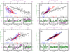 |
Fig. 3. Scatter plots of the physical quantities along the outermost azimuthal arc (i.e., penumbra) for GREGOR data (red squares), Hinode data (blue circles), and the MHD simulation (black triangles). Pearson correlations coefficients, c, for each of these pieces of data are provided in the legend. Linear fits to the data are shown with thick solid color lines. Upper left: γ − ∥B∥. Upper right: γ − Pg. Lower left: γ − ρ. Lower right: Lϕ − r−1∂Pg/∂ϕ. Each panel also includes three smaller subpanels in which the variations in the physical quantities along ϕ are displayed in purple and green colors. These subpanels are ordered as: GREGOR (left), Hinode (middle), and MHD simulations (right). This is also indicated by the arrows under the correlation coefficients for each data source. We note that the values of the ϕ components of the Lorentz force and of the gas pressure gradient in the simulations have been divided by five. |
Panel a in Fig. 3 shows a clear anticorrelation between γ and ∥B∥. It highlights the well-known uncombed structure of the penumbral magnetic field (Solanki & Montavon 1993), where regions of strong and vertical magnetic fields (γ low; ∥B∥ large) called spines alternate along the ϕ coordinate with regions of weaker and more horizontal magnetic fields (γ large; ∥B∥ low) called intraspines (Title et al. 1993; Lites et al. 1993; Martinez Pillet 1997). Panels b and c show a clear correlation in regions where the inclination of the magnetic field, γ, is larger (i.e., intraspines) and regions of enhanced gas pressure, Pg, and density, ρ. These curves indicate that the penumbral intraspines possess an excess gas pressure and density compared to the spines. This decade-long theoretical prediction (Spruit & Scharmer 2006; Scharmer & Spruit 2006; Borrero 2007) is observationally confirmed here for the first time.
Panel d in Fig. 3 shows that the gas pressure and density fluctuations, associated with the uncombed structure of the penumbral magnetic field and highlighted in panel a, are directly related to fluctuations in the azimuthal component of the Lorentz force. This is demonstrated not only by the high degree of correlation between Lϕ and r−1∂Pg/∂ϕ, but also by the fact that the slope of the scatter plot is unity, indicating that
which corresponds to the ϕ component (in cylindrical coordinates) of the MHS equilibrium equation,

where L has already been defined as the Lorentz force.
Our combined results prove that, in the azimuthal ϕ direction, penumbral spines and intraspines are in almost perfect MHS equilibrium and that neither the time derivative of the velocity, ∂v/∂t, the velocity advective term, (v ⋅ ∇)v, nor the viscosity term,  , where
  is the viscous stress tensor, play a significant role in the force balance. Interestingly, in the numerical simulations, the velocity advective term associated with the Evershed flow does indeed play an important role in the force balance in the radial direction (Rempel 2012), meaning that magnetohydrostationary equilibrium is more adequate in the radial coordinate.
It should be noted that the almost perfect MHS equilibrium in the azimuthal direction (Eq. 2) is found in the observations at short and intermediate radial distances from the center of the sunspots: r/Rspot ∈ [0.1, 0.7] (where Rspot is the radius of the sunspot) and in a height region restricted around ±150 km around the continuum τc = 1 (see Appendix A for more details). In the MHD simulations the MHS equilibrium is verified over a similar range of radial distances but over a much broader vertical region of about 400 km above τc = 1.
6.1. Contribution of the magnetic tension and magnetic pressure gradient in the Lorentz force
We have already established that the azimuthal component of the Lorentz force, Lϕ, has a one-to-one relationship to the pressure and density fluctuations in this direction seen both in observations and simulations (i.e., Eq. 2 is verified). In order to study this in more detail, we have decomposed Lϕ into the contribution from the magnetic tension, Tϕ, and from the magnetic pressure gradient, Gϕ:
where eϕ is the unit vector in the azimuthal direction. The resulting azimuthal variations in the magnetic tension and magnetic pressure gradient are shown in Figure 4. As can be seen, the similarities between the GREGOR and Hinode observations and the MHD simulations are remarkable. In all cases, the magnetic pressure gradient, Gϕ, dominates over the magnetic tension, Tϕ, with the former reaching its maximum right at the boundary between spines and intraspines, and the latter peaking at the center of the spines and intraspines, respectively.
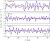 |
Fig. 4. Decomposition of the Lorentz force into magnetic pressure gradient and magnetic tension. Variations in the magnetic pressure gradient, Gϕ, (blue) and magnetic tension, Tϕ, (red) along the azimuthal coordinate, ϕ, are indicated in Fig. 2 (outermost arc) and were inferred from GREGOR (top) and Hinode (middle) observations, as well as from 3D MHD simulations (bottom). Values for the latter have been divided by a factor of five. |
6.2. Gas pressure fluctuations: Observations versus MHD simulations
In Figure 3 (panel d) we show the results of the three-dimensional MHD numerical simulations but dividing Lϕ and r−1∂Pg/∂ϕ by a factor of five so that the points of the scatter plot appear on the same scale as the ones from the GREGOR and Hinode observations. The same factor has been applied to the decomposition of the Lorentz force into the magnetic tension and gas pressure gradient contributions in Figure 4 (bottom panel). The reason for the larger values of the Lorentz force and of the gas pressure variations in the azimuthal direction in the MHD simulations is to be found in Figure 3 (panel a), in which it is shown that the MHD simulations have a much larger range of variations in the magnetic field, ∥B∥∈[2000, 3500] Gauss, compared to the observations in GREGOR and Hinode data, where ∥B∥∈[1300, 1900]. In order to demonstrate this, we take the force balance equation along the azimuthal direction (Eq. 2) and consider, as is seen in Sect. 6.1, that the main contributor to the ϕ component (azimuthal direction) of the Lorentz force is the magnetic pressure gradient in the same direction. With this, we can write
By transforming the derivatives into finite differences we can write
This demonstrates that the reason the ϕ component of the Lorentz force, and hence also the variation in the gas pressure in the azimuthal direction in the MHD simulations, is larger than in the observations is because of the larger difference in the magnetic field of the spines and intraspines in the MHD simulations. In the original (i.e., undegraded) simulation data (see left-side panels in the leftmost column in Fig. 2), the mean azimuthal distance between consecutive peaks in Pg decreases with respect to the degraded simulation data, thereby further increasing the values of Lϕ and r−1∂Pg/∂ϕ.
6.3. Results for the umbra
So far we have mostly focused on the azimuthal equilibrium of the penumbra. Following the same procedure previously described, we can also study whether the umbra satisfies the MHS equilibrium given by Lϕ = r−1∂Pg/∂ϕ. To this end, we present in Figure 5 the same study as in Figure 3 but along the innermost arc (i.e., umbral arc; Fig. 2). In panel a of Figure 5 we notice that, in the observations (red squares for Hinode and blue circles for GREGOR), the strong anticorrelation between γ − ∥B∥ is not present anymore. This was to be expected because the uncombed structure (i.e. spines and intraspines) of the penumbral magnetic field does not appear in the umbra. This is further seen in panels b and c, where positive correlations between γ − Pg and γ − ρ, respectively, are not inferred in either the Hinode or GREGOR observations.
It is important to notice that while in the penumbra the physical properties inferred from GREGOR and Hinode data are quite similar (see Fig. 3), in the umbra there are large differences between the two observed sunspots. This is particularly the case for the field strength obtained from the Stokes inversion (see a-panel in Fig. 5), with Hinode showing a larger variation in the field strength. This is likely caused by the presence of umbral dots along the innermost arc in Hinode data. The larger variation in the field strength along the ϕ coordinate then translates into a larger variation in the gas pressure and density once MHS equilibrium is taken into account.
In the MHD simulations, correlations and anticorrelations between the aforementioned physical parameters are still present, hinting at a clear presence of spines and intrapines in the simulated umbra. This was also to be expected if we attend to the innermost arc in Fig. 2 (third column). It is clear from continuum intensity and inclination maps of the MHD simulations that penumbral filaments still exist within the umbra almost up to the very center of the sunspot. This effect appears because of the time stamp, during the evolution of the sunspot, chosen for our analysis. Initially, the convection in the outer umbra shows a typical coffee-bean pattern such as the one reported in Schüssler & Vögler (2006). This pattern closely resembles the observations. However, as time passes and the cooling front goes deeper, the convection within the outer umbra no longer shows coffee beans but is more penumbra-like, with radially aligned filaments, albeit less strong and transporting less energy.
Regardless of the differences between the observed and simulated umbra, the most important fact to notice is panel d in Fig. 5, where it is still the case that in both observed and simulated umbra, the MHS equilibrium given by Eq. (2) is strongly satisfied. This demonstrates that in the azimuthal direction, the umbra is also in MHS equilibrium.
6.4. Results with vertical hydrostatic equilibrium
As is described in Section 3, as part of the inversion procedure and before the inversion with MHS constraints was applied, a first inversion under vertical HE was carried out. To study whether the inversion under vertical HE yields similar results to those under MHS equilibrium, we present in Figure C.1 the same results as in Fig. 3 but using HE instead of MHS. As can be seen, panel a in Figure C.1 still features the widely known structure of the penumbral magnetic field characterized by alternating spines and intraspines, whereby more inclined magnetic field lines (γ → 90°) are weaker than the more vertical (γ → 30°) magnetic field lines. However, the correlations between the magnetic field inclination, γ, with the gas pressure and density (panels b and c, respectively), as well as the correlations between the gas pressure variation and the Lorentz force along ϕ, are completely lost under the assumption of vertical HE. This result highlights that the conclusions presented in this paper would not have been possible unless MHS was considered.
6.5. Results without coupled inversion
In Figure C.2 we show the same results as the ones presented in Figure 3 but performing the MHS inversion using the pixel-wise inversion instead of the PSF-coupled inversion (see Sect. 3). By comparing these two figures we conclude that, although the PSF-coupled inversion is not strictly compulsory to obtain a correlation between the azimuthal component of the Lorentz force, Lϕ, and the derivative of the gas pressure in the azimuthal direction (panel d) it certainly helps to improve the correlations of the field strength, ∥B∥ (panel a), gas pressure, Pg (panel b), and density, ρ (panel c), with the inclination of the magnetic field, γ, with respect to the normal vector to the solar surface. The effects of including the PSF in the inversion are also more noticeable in the GREGOR data (ground-based) than in the Hinode data (satellite). This occurs in spite of our limited knowledge ofGREGOR’s PSF, in particular the lack of a detailed model for the seeing (see Sect. 4).
7. Conclusions
Although simplified theoretical MHS models of sunspots have been proposed in the past, those models have so far ignored the strong variations in the magnetic field in the azimuthal direction. These variations are caused not only by the filamentary structure of the penumbra but also by inhomogeneities in the umbral magnetic field caused by umbral dots and light bridges. Here we have demonstrated, using spectropolarimetric observations from both the ground and space as well as MHD simulations, that MHS equilibrium is maintained even if these azimuthal variations in the magnetic field are taken into account.
It is important to bear in mind that not all dynamic phenomena occurring at small scales in sunspots (see i.e., Section 1) are resolved at the spatial resolution of our observations, with many of them being highly relevant for the energy transport within the sunspot (Rempel & Borrero 2021). Consequently, the MHS equilibrium in the azimuthal direction unearthed by the present study might not apply at spatial scales smaller than the ones of our observations (i.e., ≤100 km Schlichenmaier et al. 2016). What can be stated, however, is that at those spatial scales these aforementioned dynamic phenomena must reach a stationary state whereby the overarching magnetic structure of the sunspot remains close to MHS (Rempel & Schlichenmaier 2011). On the other hand, we note that the undegraded MHD simulations, featuring a horizontal resolution of 32 km, verify the MHS equilibrium in the azimuthal direction with an even higher accuracy than the same simulations after degradation to the spatial resolution of the observations.
Notwithstanding their almost perfect MHS equilibrium, perturbations from this equilibrium, such as fluting instability (Meyer et al. 1977) or advective transport of the magnetic flux via moving magnetic features (Martínez Pillet 2002; Kubo et al. 2008a,b), will eventually break apart or make the sunspot decay till its eventual disappearance over long timescales.
The results presented in this work also highlight the capabilities of the FIRTEZ Stokes inversion code to infer physical parameters such as gas pressure, density, electric currents, and Lorentz force that, until now, could not be accurately determined. Gaining access to these physical parameters opens a new path to investigate the thermodynamic state and magnetic structure of the plasma in the solar atmosphere.
In this work we have not studied the equilibrium of sunspots in either the radial or vertical directions (r, z). There are several important reasons for this. On the one hand, these have already been addressed by theoretical models (Low 1975, 1980a,b; Pizzo 1986, 1990). On the other hand, the magnetic field in these two directions varies much more slowly than along ϕ (Borrero & Ichimoto 2011), and therefore the Lorentz force will likely play a less important role there. Finally, as was shown by Rempel (2012, see Fig. 22), in the radial direction in the penumbra, the velocity advective term, (v ⋅ ∇)v, associated with the Evershed flow contributes significantly to the equilibrium. This particular term cannot be considered by the FIRTEZ inversion code so far, and therefore it is not possible at this point to address the equilibrium in the radial direction employing spectropolarimetric observations.
Acknowledgments
The development of the FIRTEZ inversion code is funded by two grants from the Deutsche Forschung Gemeinschaft (DFG): projects 321818926 and 538773352. Adur Pastor acknowledges support from the Swedish Research Council (grant 2023-03313). This project has been funded by the European Union through the European Research Council (ERC) under the Horizon Europe program (MAGHEAT, grant agreement 101088184). Markus Schmassmann is supported by the Czech-German common grant, funded by the Czech Science Foundation under the project 23-07633K and by the Deutsche Forschung Gemeinschaft (DFG) under the project 511508209. Manuel Collados acknowledges financial support from Ministerio de Ciencia e Innovación and the European Regional Development Fund through grant PID2021-127487NB-I00. Matthias Rempel would like to acknowledge high-performance computing support from Cheyenne (doi:10.5065/D6RX99HX) provided by NSF NCAR’s Computational and Information Systems Laboratory (CISL), sponsored by the U.S. National Science Foundation. This material is based upon work supported by the NSF National Center for Atmospheric Research, which is a major facility sponsored by the U.S. National Science Foundation under Cooperative Agreement No. 1852977. The 1.5-m GREGOR solar telescope was built by a German consortium under the leadership of the Institut für Sonnenphysik in Freiburg with the Leibniz-Institut für Astrophysik Potsdam, the Institut für AstrophysikGöttingen, and the Max-Planck-Institut für Sonnensystemforschung in Göttingen as partners, and with contributions by the Instituto de Astrofísica de Canarias and the Astronomical Institute of the Academy of Sciences of the Czech Republic. Hinode is a Japanese mission developed and launched by ISAS/JAXA, collaborating with NAOJ as a domestic partner, NASA and STFC (UK) as international partners. Scientific operation of the Hinode mission is conducted by the Hinode science team organized at ISAS/JAXA. This team mainly consists of scientists from institutes in the partner countries. Support for the post-launch operation is provided by JAXA and NAOJ (Japan), STFC (U.K.), NASA, ESA, and NSC (Norway). This research has made use of NASA’s Astrophysics Data System. We thank an anonymous referee for suggestions that lead to important improvements on the readability of the manuscript.
References
- Anstee, S. D., & O’Mara, B. J. 1995, MNRAS, 276, 859 [Google Scholar]
- Bard, A., Kock, A., & Kock, M. 1991, A&A, 248, 315 [NASA ADS] [Google Scholar]
- Barklem, P. S., & O’Mara, B. J. 1997, MNRAS, 290, 102 [Google Scholar]
- Barklem, P. S., O’Mara, B. J., & Ross, J. E. 1998, MNRAS, 296, 1057 [Google Scholar]
- Bloomfield, D. S., Solanki, S. K., Lagg, A., Borrero, J. M., & Cally, P. S. 2007a, A&A, 469, 1155 [NASA ADS] [CrossRef] [EDP Sciences] [Google Scholar]
- Bloomfield, D. S., Lagg, A., & Solanki, S. K. 2007b, ApJ, 671, 1005 [NASA ADS] [CrossRef] [Google Scholar]
- Borrero, J. M. 2007, A&A, 471, 967 [NASA ADS] [CrossRef] [EDP Sciences] [Google Scholar]
- Borrero, J. M., & Ichimoto, K. 2011, Liv. Rev. Sol. Phys., 8, 4 [Google Scholar]
- Borrero, J. M., & Solanki, S. K. 2008, ApJ, 687, 668 [Google Scholar]
- Borrero, J. M., Bellot Rubio, L. R., Barklem, P. S., & del Toro Iniesta, J. C. 2003, A&A, 404, 749 [NASA ADS] [CrossRef] [EDP Sciences] [Google Scholar]
- Borrero, J. M., Asensio Ramos, A., Collados, M., et al. 2016, A&A, 596, A2 [NASA ADS] [CrossRef] [EDP Sciences] [Google Scholar]
- Borrero, J. M., Pastor Yabar, A., Rempel, M., & Ruiz Cobo, B. 2019, A&A, 632, A111 [NASA ADS] [CrossRef] [EDP Sciences] [Google Scholar]
- Borrero, J. M., Pastor Yabar, A., & Ruiz Cobo, B. 2021, A&A, 647, A190 [NASA ADS] [CrossRef] [EDP Sciences] [Google Scholar]
- Cabrera Solana, D., Bellot Rubio, L. R., Beck, C., & Del Toro Iniesta, J. C. 2007, A&A, 475, 1067 [NASA ADS] [CrossRef] [EDP Sciences] [Google Scholar]
- Cabrera Solana, D., Bellot Rubio, L. R., Borrero, J. M., & Del Toro Iniesta, J. C. 2008, A&A, 477, 273 [NASA ADS] [CrossRef] [EDP Sciences] [Google Scholar]
- Collados, M., López, R., Páez, E., et al. 2012, Astron. Nachr., 333, 872 [Google Scholar]
- Danilovic, S., Gandorfer, A., Lagg, A., et al. 2008, A&A, 484, L17 [NASA ADS] [CrossRef] [EDP Sciences] [Google Scholar]
- de la Cruz Rodríguez, J., Leenaarts, J., Danilovic, S., & Uitenbroek, H. 2019, A&A, 623, A74 [Google Scholar]
- Ebert, E., Milić, I., & Borrero, J. M. 2024, A&A, 691, A176 [NASA ADS] [CrossRef] [EDP Sciences] [Google Scholar]
- Falco, M., Borrero, J. M., Guglielmino, S. L., et al. 2016, Sol. Phys., 291, 1939 [Google Scholar]
- Franz, M., & Schlichenmaier, R. 2013, A&A, 550, A97 [EDP Sciences] [Google Scholar]
- Franz, M., Collados, M., Bethge, C., et al. 2016, A&A, 596, A4 [Google Scholar]
- Frutiger, C., Solanki, S. K., Fligge, M., & Bruls, J. H. M. J. 1999, Astrophys. Space Sci. Lib., 243, 281 [NASA ADS] [CrossRef] [Google Scholar]
- Georgoulis, M. K. 2005, ApJ, 629, L69 [Google Scholar]
- Golub, G., & Kahan, W. 1965, SIAM J. Numer. Anal., 2, 205 [Google Scholar]
- Ichimoto, K., Suematsu, Y., Tsuneta, S., et al. 2007a, Science, 318, 1597 [NASA ADS] [CrossRef] [Google Scholar]
- Ichimoto, K., Suematsu, Y., Shimizu, T., et al. 2007b, ASP Conf. Ser., 369, 39 [NASA ADS] [Google Scholar]
- Jahn, K., & Schmidt, H. U. 1994, A&A, 290, 295 [NASA ADS] [Google Scholar]
- Jurčák, J., Schmassmann, M., Rempel, M., Bello González, N., & Schlichenmaier, R. 2020, A&A, 638, A28 [NASA ADS] [CrossRef] [EDP Sciences] [Google Scholar]
- Khomenko, E., & Collados, M. 2008, ApJ, 689, 1379 [NASA ADS] [CrossRef] [Google Scholar]
- Kosugi, T., Matsuzaki, K., Sakao, T., et al. 2007, Sol. Phys., 243, 3 [Google Scholar]
- Kubo, M., Lites, B. W., Ichimoto, K., et al. 2008a, ApJ, 681, 1677 [Google Scholar]
- Kubo, M., Lites, B. W., Shimizu, T., & Ichimoto, K. 2008b, ApJ, 686, 1447 [Google Scholar]
- Lites, B. W., Elmore, D. F., Seagraves, P., & Skumanich, A. P. 1993, ApJ, 418, 928 [NASA ADS] [CrossRef] [Google Scholar]
- Lites, B. W., Elmore, D. F., & Streander, K. V. 2001, ASP Conf. Ser., 236, 33 [NASA ADS] [Google Scholar]
- Löhner-Böttcher, J., & Bello González, N. 2015, A&A, 580, A53 [NASA ADS] [CrossRef] [EDP Sciences] [Google Scholar]
- Low, B. C. 1975, ApJ, 197, 251 [NASA ADS] [CrossRef] [Google Scholar]
- Low, B. C. 1980a, Sol. Phys., 65, 147 [NASA ADS] [CrossRef] [Google Scholar]
- Low, B. C. 1980b, Sol. Phys., 67, 57 [Google Scholar]
- Martinez Pillet, V. 1997, ASP Conf. Ser., 118, 212 [Google Scholar]
- Martínez Pillet, V. 2002, Astron. Nachr., 323, 342 [Google Scholar]
- Mathew, S. K., Lagg, A., Solanki, S. K., et al. 2003, A&A, 410, 695 [NASA ADS] [CrossRef] [EDP Sciences] [Google Scholar]
- Metcalf, T. R., Leka, K. D., Barnes, G., et al. 2006, Sol. Phys., 237, 267 [Google Scholar]
- Meyer, F., Schmidt, H. U., & Weiss, N. O. 1977, MNRAS, 179, 741 [NASA ADS] [Google Scholar]
- Nave, G., Johansson, S., Learner, R. C. M., Thorne, A. P., & Brault, J. W. 1994, ApJS, 94, 221 [Google Scholar]
- Orozco Suárez, D., Quintero Noda, C., Ruiz Cobo, B., Collados Vera, M., & Felipe, T. 2017, A&A, 607, A102 [NASA ADS] [CrossRef] [EDP Sciences] [Google Scholar]
- Ortiz, A., Bellot Rubio, L. R., & Rouppe van der Voort, L. 2010, ApJ, 713, 1282 [Google Scholar]
- Panja, M., Cameron, R., & Solanki, S. K. 2020, ApJ, 893, 113 [CrossRef] [Google Scholar]
- Pizzo, V. J. 1986, ApJ, 302, 785 [NASA ADS] [CrossRef] [Google Scholar]
- Pizzo, V. J. 1990, ApJ, 365, 764 [Google Scholar]
- Press, W. H., Flannery, B. P., & Teukolsky, S. A. 1986, Numerical Recipes. The Art of Scientific Computing (Cambridge: Cambridge University Press) [Google Scholar]
- Rempel, M. 2011, ApJ, 729, 5 [Google Scholar]
- Rempel, M. 2012, ApJ, 750, 62 [Google Scholar]
- Rempel, M., & Borrero, J. 2021, Oxford Research Encyclopedia of Physics (Oxford University Press) [Google Scholar]
- Rempel, M., & Schlichenmaier, R. 2011, Liv. Rev. Sol. Phys., 8, 3 [Google Scholar]
- Rempel, M., Schüssler, M., Cameron, R. H., & Knölker, M. 2009a, Science, 325, 171 [CrossRef] [Google Scholar]
- Rempel, M., Schüssler, M., & Knölker, M. 2009b, ApJ, 691, 640 [Google Scholar]
- Rogers, F. J., Swenson, F. J., & Iglesias, C. A. 1996, ApJ, 456, 902 [Google Scholar]
- Ruiz Cobo, B., & del Toro Iniesta, J. C. 1992, ApJ, 398, 375 [Google Scholar]
- Scharmer, G. B., & Spruit, H. C. 2006, A&A, 460, 605 [NASA ADS] [CrossRef] [EDP Sciences] [Google Scholar]
- Scharmer, G. B., Henriques, V. M. J., Kiselman, D., & de la Cruz Rodríguez, J. 2011, Science, 333, 316 [Google Scholar]
- Schlichenmaier, R., von der Lühe, O., Hoch, S., et al. 2016, A&A, 596, A7 [NASA ADS] [CrossRef] [EDP Sciences] [Google Scholar]
- Schlüter, A., & Temesváry, S. 1958, IAU Symp., 6, 263 [Google Scholar]
- Schmassmann, M., Rempel, M., Bello González, N., Schlichenmaier, R., & Jurčák, J. 2021, A&A, 656, A92 [NASA ADS] [CrossRef] [EDP Sciences] [Google Scholar]
- Schmidt, W., von der Lühe, O., Volkmer, R., et al. 2012, Astron. Nachr., 333, 796 [Google Scholar]
- Schüssler, M., & Rempel, M. 2005, A&A, 441, 337 [NASA ADS] [CrossRef] [EDP Sciences] [Google Scholar]
- Schüssler, M., & Vögler, A. 2006, ApJ, 641, L73 [Google Scholar]
- Shimizu, T., Nagata, S., Tsuneta, S., et al. 2008, Sol. Phys., 249, 221 [Google Scholar]
- Sobotka, M., & Jurčák, J. 2009, ApJ, 694, 1080 [Google Scholar]
- Socas-Navarro, H., de la Cruz Rodríguez, J., Asensio Ramos, A., Trujillo Bueno, J., & Ruiz Cobo, B. 2015, A&A, 577, A7 [NASA ADS] [CrossRef] [EDP Sciences] [Google Scholar]
- Solanki, S. K. 2003, A&ARv, 11, 153 [Google Scholar]
- Solanki, S. K., & Montavon, C. A. P. 1993, A&A, 275, 283 [NASA ADS] [Google Scholar]
- Spruit, H. C., & Scharmer, G. B. 2006, A&A, 447, 343 [NASA ADS] [CrossRef] [EDP Sciences] [Google Scholar]
- Stanchfield, D. C. H., II, Thomas, J. H., & Lites, B. W. 1997, ApJ, 477, 485 [Google Scholar]
- Suematsu, Y., Tsuneta, S., Ichimoto, K., et al. 2008, Sol. Phys., 249, 197 [Google Scholar]
- Title, A. M., Frank, Z. A., Shine, R. A., et al. 1993, ApJ, 403, 780 [NASA ADS] [CrossRef] [Google Scholar]
- Tsuneta, S., Ichimoto, K., Katsukawa, Y., et al. 2008, Sol. Phys., 249, 167 [Google Scholar]
- van der Vorst, H. A. 1992, SIAM J. Sci. Stat. Comput., 13, 631 [CrossRef] [Google Scholar]
- van Noort, M. 2012, A&A, 548, A5 [NASA ADS] [CrossRef] [EDP Sciences] [Google Scholar]
- Vögler, A., Shelyag, S., Schüssler, M., et al. 2005, A&A, 429, 335 [Google Scholar]
Appendix A: Do MHS inversions enforce ∇Pg = L?
Since the MHS inversions carried out with the FIRTEZ Stokes inversion code take into account the Lorentz force, it is natural to wonder whether our observational results verify r−1∂Pg/∂ϕ = Lϕ as a consequence of being internally imposed. In order to answer this question, it is convenient to take a step back and first study the implications of having HE. Full (i.e., in 3D) HE is obtained by neglecting the Lorentz force (L = 0 in Eq. 3). The resulting equation can be decomposed in:

With the exception of the FIRTEZ code, all Stokes inversion codes such as SIR (Ruiz Cobo & del Toro Iniesta 1992), SPINOR (Frutiger et al. 1999), STiC (de la Cruz Rodríguez et al. 2019), NICOLE (Socas-Navarro et al. 2015), etc. consider only Eq. A.2 (i.e., vertical HE), but they neglect that there is also horizontal HE (Eqs. A.1) that implies that the gas pressure cannot vary in planes of constant z:

Consequently, two pixels on the solar surface, sitting next to each other (on the XY plane) must have the same Pg(z). This must be satisfied ∀z’s. Next, by applying Eq. A.2, we can also conclude that all pixels on the XY plane must have the same density ρ(z), and therefore also the same temperature T(z). In other words, neither ρ, Pg nor T can depend on (x, y). Now, we must take into account that typically from the inversion of the Stokes vector we obtain T(x, y, z). This immediately implies that horizontal HE cannot be maintained in the sense that Eqs. A.1 and A.2 cannot be simultaneously satisfied. Hence Eq. A.1 is usually ignored and only Eq. A.2 is considered, hence the term vertical HE.
Now, as explained in Borrero et al. (2019), FIRTEZ does not directly solve the momentum equation in MHS (Eq. 3). Instead, it takes the divergence of that equation and iteratively solves the following second-order Poisson equation:
![$$ \begin{aligned} \nabla ^2 (\ln P_{\rm g}) = -\frac{m_a g}{K_b} \frac{\partial }{\partial z}\left[\frac{u}{T}\right] + \nabla \cdot \left(\frac{\mathbf{L }^{\prime }}{P_{\rm g}}\right) \end{aligned} $$](/articles/aa/full_html/2025/07/aa54241-25/aa54241-25-eq13.gif)
where L′ is a modified Lorentz force. Let us leave L′ aside for the moment and ask ourselves what does FIRTEZ do when the Lorentz force is neglected (i.e., HE). Under this assumption FIRTEZ solves:
![$$ \begin{aligned} \nabla ^2 (\ln P_{\rm g}) = - \frac{m_a g}{K_b} \frac{\partial }{\partial z}\left[\frac{u}{T}\right] \end{aligned} $$](/articles/aa/full_html/2025/07/aa54241-25/aa54241-25-eq14.gif)
But let us now remember that typically the inversion will yield T(x, y, z) and hence also a variable mean molecular weight u(x, y, z), so the that the term:
![$$ \begin{aligned} \frac{\partial }{\partial z}\left[\frac{u}{T}\right] = f(x,y,z) \end{aligned} $$](/articles/aa/full_html/2025/07/aa54241-25/aa54241-25-eq15.gif)
And consequently, the resulting Pg from solving Eq. A.5 will also be a function of (x, y, z). But this is contradictory with HE as we just saw above because full 3D HE implies Pg = f(z) only.
So, it is clear that the method FIRTEZ employs to retrieve the gas pressure will result in Pg = f(x, y, z) even if L′ = 0 and thus, the fact that Pg changes horizontally (i.e., along ϕ), is not necessarily due to the Lorentz force. In fact, there is no guarantee that the following equation:

must be satisfied always at all points of the three-dimensional domain. In order to prove this particular point, the top panels on Figure A.1 show the correlations between the right-hand side and left-hand side of Eq. A.7 as a function of (r, z) in the observed and simulated sunspots.
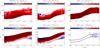 |
Fig. A.1. Study of the MHS equilibrium along the azimuthal direction for the whole sunspots. Top panels: Pearson’s correlation coefficient between the rhs and lhs of Eq. A.7 as a function of (r, z). Bottom panels: same as on the top but for the slope of the linear regression between the rhs and lhs of Eq. A.7 as a function of (r, z). Rs represents the radius of the sunspots. Solid black lines show the ϕ-average location of the τc = 1, 10−2. Observational results are displayed on the left (GREGOR) and middle (Hinode) panels. Results from the MHD simulations are presented in the rightmost panels. |
Figure A.1 shows that although the correlations are large in the observations (left and middle panels for GREGOR and Hinode, respectively), this is certainly not always the case. In fact there are regions where the obtained correlation is actually negative. Such is the case of the high photosphere at all radial distances, and of the mid-photosphere at short radial distances (i.e., in the umbra). For comparison the simulated sunspot is also displayed in the rightmost panel. Here we can see that the MHD simulations show a high degree of correlation over a wider range of radial distances r/Rspot and heights z.
On the other hand, a high correlation between the rhs and lhs side of Eq. A.7 does not necessarily mean that this equation is strictly fulfilled. It can occur that they are correlated but not necessarily equal. We have evaluated this by performing a linear fit to the scatter plot of Lϕ and r−1∂Pg/∂ϕ (as done in panel d of Fig. 3) and plotting on the bottom panels of Figure A.1, the slope m of the linear fit between the rhs and the lhs of Eq. A.7 as a function of (r, z).
Figure A.1 (bottom-right and bottom-middle panels) shows that even though there might be very high correlations between the two terms on either side of Eq. A.7 the actual equation is strictly fulfilled only in the region where the slope is close to 1.0, that is, in a narrow region of the observed sunspots around the τc = 1 level. This is in contrast with the sunspot simulated with the MuRAM code, where Eq. A.7 is verified to a large degree (i.e., slope 1.0) over a much wider region, both vertically and radially, than in the observations analyzed with the FIRTEZ code. Because of these results it is possible to state that Eq. A.7 is not strictly imposed by FIRTEZ.
The question now arises to what extent we can expect Eq. A.7 to be strictly fulfilled. As explained above, T(x, y, z) implies that full 3D HE cannot be fulfilled by FIRTEZ even if the Lorentz force is zero. This can be also interpreted in the following way: since under HE (i.e., L′ = 0) T and Pg can only a function of z, the fact that FIRTEZ receives T(x, y, z) already implies the presence of a residual force not given by (∇×B)×B (i.e., the Lorentz force) so that the resulting gas pressure also depends on (x, y, z).
The nature of the aforementioned residual force can be understood by looking at the right-hand-side of Eq. A.4. Here, after defining F = L′/Pg and projecting onto its Hodge’s components: F = ∇Ψ + ∇ × W, we see that Eq. A.4 becomes:
![$$ \begin{aligned} \nabla ^2 (\ln P_{\rm g}) = - \frac{m_a g}{K_b} \frac{\partial }{\partial z}\left[\frac{u}{T}\right] + \nabla ^2 \Psi \end{aligned} $$](/articles/aa/full_html/2025/07/aa54241-25/aa54241-25-eq17.gif)
where it is clear now that in the presence of a magnetic field, FIRTEZ infers a gas pressure Pg that balances the potential part Ψ of the force F = L′/Pg with the residual forces being identified with the non-potential part W of this force.
Therefore, one can expect the results from the FIRTEZ code to fulfill Eq. A.7 when the potential part of the L′/Pg actually dominates over its non-potential component. Otherwise it is conceivable that the potential component will still be capable of introducing a correlation between Lϕ and r−1∂Pg/∂ϕ but the slope of the linear fit between these two quantities might be quite different from 1.0 (see Fig. A.1).
It is now time to remember that the modified Lorentz force L′ used by FIRTEZ to determine the gas pressure via the solution of Eq. A.4 is not necessarily the Lorentz force obtained via the inferred magnetic field. Instead, FIRTEZ takes the calculated electric current j = c(4π)−1∇×B and dampens it by a factor ∝β2 (with β being the ratio between magnetic and gas pressure) whenever the module ∥j∥ exceeds a maximum allowed value. This is done with the aim that, in the upper atmosphere where the β ≪ 1 and where spectral lines do not convey accurate values of magnetic field B, electric currents determined from these inaccurate magnetic fields do not dominate the force balance. This explains why the agreement of the observational results with Eq. A.7 worsens progressively from the lower atmosphere towards the upper atmosphere (see Fig. A.1). This effect reinforces the previous conclusion that the MHS equilibrium imposed by FIRTEZ does not strictly impose Eq. A.7.
Appendix B: Simulation details
The initial magnetic field of the simulation uses the self-similar approach used in Schlüter & Temesváry (1958) and others:

whereby Bz is the vertical component of the magnetic field, Br the radial component, r the distance from the spot axis, and z the distance from the bottom of the box. For this simulation
The parameters are B0 = 6.4 kG, the initial field strength on the spot axis at the bottom of the box, R0 = 8.2 Mm and z0 = 6.4185 Mm, which determines how far away from the axis and the bottom Bz reduces by a factor e. These parameters lead to a sunspot with an initial flux of F0 = 1.2 × 10²² Mx and a field strength at the top of 2.56 kG. A more detailed description of the initial state of the simulation is in Rempel (2012). Other self-similar sunspot models use for f(ξ) a Gaussian (e.g. Schlüter & Temesváry 1958; Schüssler & Rempel 2005) or the boxcar function (many analytical models and e.g. Panja et al. 2020) and g(z) is sometimes related to the pressure difference between the spot center and the quiet Sun (e.g. Schlüter & Temesváry 1958).
The parameter α = 2 means that at the top of the box, the horizontal field is twice what it would be if potential extrapolation were employed:
and
whereby Bz, 0 is the vertical field at the top of the box, z the height above the top of the box (in the ghost cells), ℱ the horizontal Fourier transform, kx the Fourier modes, and  . For By holds the same equation as Eq. B.7 but performing the substitution kx → ky. α > 1 is responsible for Br being larger than in the simulated penumbra compared toobservations.
For a comparison to observed sunspots, see Jurčák et al. (2020), which concludes that in sunspots with α > 1 have a too low Bz at the umbral boundary. Furthermore, Schmassmann et al. (2021) conclude, that a sufficiently strong Bz suppresses penumbral-type overturning convection.
Appendix C: Additional results
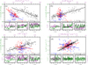 |
Fig. C.1. Same as Figure 3 but obtained under the assumption of vertical HE (see Sect. 6.4). Results from MHD simulations (black colors and rightmost minipanels) are identical to Fig. 3. |
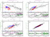 |
Fig. C.2. Same as Figure 3 but obtained without horizontal coupling between the pixels due to the telescope’s PSF (see Sect. 6.5). Results from MHD simulations (black colors and rightmost minipanels) are identical to Fig. 3. |
All Tables
All Figures
|
Fig. 1. Point spread functions employed in the data analysis. Left panel: PSF (diffraction-limited plus seeing) used in the coupled-inversion of GREGOR/GRIS data. Middle panel: PSF (diffraction-limited) used in the coupled-inversion of Hinode/SP data. For both GREGOR and Hinode data, the full PSF (±1.6 Mm) was used in the synthesis, whereas in the inversion only the square box was considered. Right panel: Ideal PSF (Airy function) used to degrade the MHD simulations. |
| In the text | |
|
Fig. 2. Summary of analyzed data and inversion results. Top row: Continuum intensity normalized to the average quiet Sun intensity, Ic/Ic, qs. Middle row: Temperature, T. Bottom row: Inclination of the magnetic field, γ, with respect to the normal vector to the solar surface. All values were taken at the continuum optical depth, τc = 1. Left column: Sunspot observed with the ground telescope GREGOR and data inverted with the FIRTEZ code. Middle column: Same as before but for the sunspot recorded with the Hinode satellite. Right column: Sunspot simulated with the MuRAM code. Each panel is split on two: the left side of the first two columns display the results of the pixel-wise Stokes inversion, whereas the right side presents the results of the PSF-coupled inversion. In the third column, the left side shows the simulation with the original horizontal resolution of 32 km × 32 km, while the right side shows the simulation convolved and resampled to 128 km × 128 in order to match the approximate resolution and sampling of the GREGOR and Hinode data. Each figure contains the direction of the center of the solar disk (blue arrow) and displays two azimuthal paths with a varying angle, ϕ, at a constant radial distance from the spots’ center: the outermost arc is in the penumbra, whereas the innermost arc lies in the umbra. |
| In the text | |
|
Fig. 3. Scatter plots of the physical quantities along the outermost azimuthal arc (i.e., penumbra) for GREGOR data (red squares), Hinode data (blue circles), and the MHD simulation (black triangles). Pearson correlations coefficients, c, for each of these pieces of data are provided in the legend. Linear fits to the data are shown with thick solid color lines. Upper left: γ − ∥B∥. Upper right: γ − Pg. Lower left: γ − ρ. Lower right: Lϕ − r−1∂Pg/∂ϕ. Each panel also includes three smaller subpanels in which the variations in the physical quantities along ϕ are displayed in purple and green colors. These subpanels are ordered as: GREGOR (left), Hinode (middle), and MHD simulations (right). This is also indicated by the arrows under the correlation coefficients for each data source. We note that the values of the ϕ components of the Lorentz force and of the gas pressure gradient in the simulations have been divided by five. |
| In the text | |
|
Fig. 4. Decomposition of the Lorentz force into magnetic pressure gradient and magnetic tension. Variations in the magnetic pressure gradient, Gϕ, (blue) and magnetic tension, Tϕ, (red) along the azimuthal coordinate, ϕ, are indicated in Fig. 2 (outermost arc) and were inferred from GREGOR (top) and Hinode (middle) observations, as well as from 3D MHD simulations (bottom). Values for the latter have been divided by a factor of five. |
| In the text | |
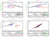 |
Fig. 5. Same as Figure 3 but in the umbra (i.e., innermost arc in Fig. 2). |
| In the text | |
|
Fig. A.1. Study of the MHS equilibrium along the azimuthal direction for the whole sunspots. Top panels: Pearson’s correlation coefficient between the rhs and lhs of Eq. A.7 as a function of (r, z). Bottom panels: same as on the top but for the slope of the linear regression between the rhs and lhs of Eq. A.7 as a function of (r, z). Rs represents the radius of the sunspots. Solid black lines show the ϕ-average location of the τc = 1, 10−2. Observational results are displayed on the left (GREGOR) and middle (Hinode) panels. Results from the MHD simulations are presented in the rightmost panels. |
| In the text | |
|
Fig. C.1. Same as Figure 3 but obtained under the assumption of vertical HE (see Sect. 6.4). Results from MHD simulations (black colors and rightmost minipanels) are identical to Fig. 3. |
| In the text | |
|
Fig. C.2. Same as Figure 3 but obtained without horizontal coupling between the pixels due to the telescope’s PSF (see Sect. 6.5). Results from MHD simulations (black colors and rightmost minipanels) are identical to Fig. 3. |
| In the text | |
Current usage metrics show cumulative count of Article Views (full-text article views including HTML views, PDF and ePub downloads, according to the available data) and Abstracts Views on Vision4Press platform.
Data correspond to usage on the plateform after 2015. The current usage metrics is available 48-96 hours after online publication and is updated daily on week days.
Initial download of the metrics may take a while.