| Issue |
A&A
Volume 699, July 2025
|
|
|---|---|---|
| Article Number | A168 | |
| Number of page(s) | 12 | |
| Section | Numerical methods and codes | |
| DOI | https://doi.org/10.1051/0004-6361/202453388 | |
| Published online | 07 July 2025 | |
Uncertainty estimation for time series classification
Exploring predictive uncertainty in transformer-based models for variable stars
1
Department of Computer Science, Universidad de Concepción,
Edmundo Larenas 219,
Concepción,
Chile
2
John A. Paulson School of Engineering and Applied Sciences, Harvard University,
Cambridge,
MA
02138,
USA
3
Center for Data and Artificial Intelligence, Universidad de Concepción,
Edmundo Larenas 310,
Concepción,
Chile
4
Millennium Institute of Astrophysics (MAS),
Nuncio Monseñor Sotero Sanz 100, Of. 104, Providencia,
Santiago,
Chile
5
Millennium Nucleus on Young Exoplanets and their Moons (YEMS),
Chile
6
Heidelberg Institute for Theoretical Studies, Heidelberg,
Baden-Württemberg,
Germany
⋆ Corresponding authors: This email address is being protected from spambots. You need JavaScript enabled to view it.
;This email address is being protected from spambots. You need JavaScript enabled to view it.
Received:
11
December
2024
Accepted:
30
April
2025
Abstract
Context. Classifying variable stars is key to understanding stellar evolution and galactic dynamics. With the demands of large astronomical surveys, machine learning models, especially attention-based neural networks, have become the state of the art. While achieving high accuracy is crucial, improving model interpretability and uncertainty estimation is equally important to ensuring that insights are both reliable and comprehensible.
Aims. We aim to enhance transformer-based models for classifying astronomical light curves by incorporating uncertainty estimation techniques to detect misclassified instances. We tested our methods on labeled datasets from MACHO, OGLE-III, and ATLAS, introducing a framework that significantly improves the reliability of automated classification for next-generation surveys.
Methods. We used Astromer, a transformer-based encoder designed to capture representations of single-band light curves. We enhanced its capabilities by applying three methods for quantifying uncertainty: Monte Carlo dropout (MC Dropout), hierarchical stochastic attention, and a novel hybrid method that combines the two approaches (HA-MC Dropout). We compared these methods against a baseline of deep ensembles. To estimate uncertainty scores for the misclassification task, we used the following uncertainty estimates: the sampled maximum probability, probability variance (PV), and Bayesian active learning by disagreement.
Results. In predictive performance tests, HA-MC Dropout outperforms the baseline, achieving macro F1-scores of 79.8 ± 0.5 on OGLE, 84 ± 1.3 on ATLAS, and 76.6 ± 1.8 on MACHO. When comparing the PV score values, the quality of uncertainty estimation by HA-MC Dropout surpasses that of all other methods, with improvements of 2.5 ± 2.3 for MACHO, 3.3 ± 2.1 for ATLAS, and 8.5 ± 1.6 for OGLE-III.
Key words: methods: analytical / methods: data analysis / methods: statistical / stars: variables: general
© The Authors 2025
 Open Access article, published by EDP Sciences, under the terms of the Creative Commons Attribution License (https://creativecommons.org/licenses/by/4.0), which permits unrestricted use, distribution, and reproduction in any medium, provided the original work is properly cited.
This article is published in open access under the Subscribe to Open model. This email address is being protected from spambots. You need JavaScript enabled to view it. to support open access publication.
1 Introduction
The identification and classification of variable stars is crucial to advancing our understanding of the cosmos. For example, Cepheids and RR Lyrae stars are key rungs on the cosmological distance ladder (Feast et al. 2014; Ngeow 2015). The emergence of next-generation survey telescopes, such as the Vera Rubin Observatory and its Legacy Survey of Space and Time (LSST; Ivezić et al. 2019), presents new opportunities for analyzing an abundance of photometric observations. Such comprehensive data, with their corresponding timestamps (i.e., light curves), are instrumental for detecting new classes of variable stars and uncovering previously unknown astronomical phenomena (Bassi et al. 2021).
Classifying light curves is essential for analyzing variable stars; however, this task presents significant challenges due to heteroskedasticity, sparsity, and observational gaps (Mahabal et al. 2017). Astronomy has transitioned from traditional feature-based analysis to advanced data-driven models enabled by deep learning (Smith & Geach 2023). This evolution is evidenced by the adoption of diverse architectures ranging from multilayer perceptrons (Karpenka et al. 2013) to recurrent neural networks and convolutional neural networks (Cabrera-Vives et al. 2016; Mahabal et al. 2017; Protopapas 2017; Naul et al. 2018; Carrasco-Davis et al. 2019; Becker et al. 2020; Donoso-Oliva et al. 2021).
Building upon this evolution, self-attention-based models are setting new benchmarks (Donoso-Oliva et al. 2023; Moreno-Cartagena et al. 2023; Pan et al. 2024; Leung & Bovy 2023; Parker et al. 2024). These models have various applications, from inferring black hole properties (Park et al. 2021) to denoising light curves (Morvan et al. 2022) and specialized multiband light-curve classification (Pimentel et al. 2022; Cabrera-Vives et al. 2024).
As the complexity of models escalates, ensuring the reliability of classification results becomes increasingly critical. Within the framework of deep neural networks, uncertainty estimation is pivotal, as it not only increases the confidence in predictions but also proves particularly beneficial in the detection of misclassifications, where uncertain predictions can signal potential errors (Gawlikowski et al. 2023). Traditional techniques such as Bayesian neural networks (Blundell et al. 2015), which inherently model uncertainty by approximating a posterior distribution over model parameters, have been effective in astronomy (Möller & de Boissière 2020; Killestein et al. 2021; Ciucă et al. 2021). However, their training stage requires a high computational capacity, leading to increased resource use and extended convergence times.
In this work, we present a methodology that combines deep attention-based classifiers with uncertainty estimation techniques for misclassification detection. Our model is based on Astromer, the transformer-based embedding approach proposed by Donoso-Oliva et al. (2023). For our analysis, we implemented three state-of-the-art uncertainty estimation approaches: deep ensembles (DEs; Valdenegro-Toro 2019; Ganaie et al. 2022), Monte Carlo dropout (MC Dropout; Gal & Ghahramani 2016), and hierarchical stochastic attention (HSA; Pei et al. 2022). We additionally propose an alternative approach, hierarchical attention with MC dropout (HA-MC Dropout), which integrates a hierarchical attention structure with dropout activation during the inference stage.
Although DEs are computationally expensive in practice, they establish a robust baseline for capturing uncertainty and facilitate comparisons with other techniques (Lakshminarayanan et al. 2017). Thus, we used DEs as a baseline to compare the performance of MC Dropout, HSA, and HA-MC Dropout within a variable star transformer-based classifier.
We further assessed the uncertainty estimation capabilities of our models through statistical significance tests. Notably, we present a methodology that fuses deep attention-based classifiers for astronomical time series with uncertainty estimation techniques. Furthermore, we establish through empirical evaluations that the HA-MC Dropout approach outperforms DEs in the context of variable star classification, emphasizing its utility as a primary technique for this application.
This work is organized as follows: Section 2 details the attention-based architecture and the methods we employed, and formally defines the evaluation techniques used in our research. Section 3 presents the experimental setup, including dataset descriptions and the generation of misclassification instances. Our findings are then introduced in Sect. 4, and the paper concludes with Sect. 5, which summarizes the key outcomes and insights derived from our work.
2 Methods
This section presents the methodology adopted in our work, focusing on the Astromer transformer-based model and its integration of uncertainty estimation techniques. Our work involves the following aspects:
Injecting stochasticity to the model using the following methods: DEs (Sect. 2.2), MC Dropout (Sect. 2.3), HSA (Sect. 2.4), and HA-MC Dropout (Sect. 2.5).
Interpret uncertainty through uncertainty estimation scores (Sect. 2.6).
Evaluating the quality of the uncertainty estimated by each model based on their ability to identify misclassified instances (Sect. 2.7).
We describe the four principal approaches: DEs, MC Dropout, HSA, and HA-MC Dropout to assess predictive uncertainty. Additionally, we explain the three types of uncertainty estimates (UEs) employed for the misclassification task and outline the methodology for quality evaluation.
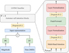 |
Fig. 1 Astromer architecture diagram with the LSTM classifier on top. |
2.1 Transformer-based model for light curves
Our work uses an architecture inspired by Astromer, which is an encoder-decoder model derived from the principles of the bidirectional encoder representations from transformers (BERT; Devlin et al. 2019). Unlike BERT, which is specifically designed for natural language processing (NLP) tasks, Astromer is adapted for capturing embedding representations of astronomical light curves, serving as an automatic feature extractor for these time series. The model diagram is shown in Fig. 1.
The model includes several key components: positional encoding (PE), two self-attention blocks, and a long-short-term memory network (LSTM) classifier (Hochreiter & Schmidhuber 1997). It processes single-band time series, each consisting of L = 200 observations. These observations are characterized by a vector of magnitudes, x ∈ ℝL, and corresponding timestamps, t ∈ ℝL. The PE component encodes each timestamp using trigonometric functions, similar to those defined in Vaswani et al. (2017); however, it operates in the time domain of the light curve, rather than using index positions. Simultaneously, the magnitude data are fed into a feed-forward (FF) neural network. For each point in the light curve, both the PE and the FF neural network output a vector of dimensionality dx = 256. The outputs from the PE and the magnitudes FF neural network are added to produce X ∈ ℝL×dx. This 200 × 256 matrix serves as the input representation for the standard transformer self-attention mechanism.
Transformers are composed of multiple layers of self-attention heads. A self-attention head transforms X into query, key, and value matrices (Q, K, V) by using trainable weights WQ, WK, WV ∈ ℝdx × dk:
![Mathematical equation: $\[\mathbf{Q=X W_Q, \quad K=X W_K, \quad V=X W_V,}\]$](/articles/aa/full_html/2025/07/aa53388-24/aa53388-24-eq1.png) (1)
(1)
where dk is the dimension of the output of the attention head for each observation.
Attention weights αi,j represent how much token i attends token j. These weights are determined by calculating the dot product between the query and key vectors, ![Mathematical equation: $\[\boldsymbol{q}_{i}=\boldsymbol{W}_{Q}^{\top} \boldsymbol{x}_{i}\]$](/articles/aa/full_html/2025/07/aa53388-24/aa53388-24-eq2.png) and
and ![Mathematical equation: $\[\boldsymbol{k}_{j}=\boldsymbol{W}_{\boldsymbol{K}}^{\top} \boldsymbol{x}_{j}\]$](/articles/aa/full_html/2025/07/aa53388-24/aa53388-24-eq3.png) , and passing them through a softmax function in order to normalize them. Here, xi represents the i-th row of X. To stabilize the gradients during training, the dot product is divided by the square root of the dimension of the key vectors
, and passing them through a softmax function in order to normalize them. Here, xi represents the i-th row of X. To stabilize the gradients during training, the dot product is divided by the square root of the dimension of the key vectors ![Mathematical equation: $\[\sqrt{d}\]$](/articles/aa/full_html/2025/07/aa53388-24/aa53388-24-eq4.png) . In other words,
. In other words,
![Mathematical equation: $\[\begin{aligned}\boldsymbol{\alpha}_i & =\operatorname{softmax}\left(\frac{\boldsymbol{q}_i^{\top} \boldsymbol{k}_1}{\sqrt{d_k}}, \frac{\boldsymbol{q}_i^{\top} \boldsymbol{k}_2}{\sqrt{d_k}}, \cdots, \frac{\boldsymbol{q}_i^{\top} \boldsymbol{k}_L}{\sqrt{d_k}}\right), \\& =\operatorname{softmax}\left(\boldsymbol{K} \boldsymbol{q}_i\right).\end{aligned}\]$](/articles/aa/full_html/2025/07/aa53388-24/aa53388-24-eq5.png) (2)
(2)
The output hi for each head is computed by applying the normalized attention weights to the corresponding values ![Mathematical equation: $\[\boldsymbol{v}_{i}= \boldsymbol{W}_{\boldsymbol{V}}^{\top} \boldsymbol{x}_{i}\]$](/articles/aa/full_html/2025/07/aa53388-24/aa53388-24-eq6.png) :
:
![Mathematical equation: $\[\boldsymbol{h}_i=\sum_j \alpha_{i, j} \boldsymbol{v}_j.\]$](/articles/aa/full_html/2025/07/aa53388-24/aa53388-24-eq7.png) (3)
(3)
In other words, the output of each head is the sum of the value vector representation of the input weighted by the attention paid to each of these vectors. This is usually written as
![Mathematical equation: $\[\operatorname{Attention}(\boldsymbol{Q}, \boldsymbol{K}, \boldsymbol{V})=\operatorname{softmax}\left(\frac{\boldsymbol{Q} \boldsymbol{K}^{\top}}{\sqrt{d_k}}\right) \boldsymbol{V},\]$](/articles/aa/full_html/2025/07/aa53388-24/aa53388-24-eq8.png) (4)
(4)
where the softmax is applied row-wise.
After calculating the outputs hi of each head, they are concatenated [h1, . . ., h#heads] and then projected through a learned linear transformation WO ∈ ℝdx×dx, which combines information from all heads and ensures that the output maintains the expected model dimensionality dx. This transformation produces the final output of the multi-head attention block, which is then passed to subsequent layers. Figure 2 shows a graphical representation of the multi-head attention mechanism described.
Astromer has two blocks, each consisting of four heads with 64 neurons. To mitigate overfitting, it incorporates five dropout layers with a rate of 0.1. The output from this encoder is then fed into a two-layer LSTM network, which uses a softmax activation function to perform classification.
We initialized our encoders with pretrained weights provided by the authors, who pretrained Astromer using 1 529 386 R-band light curves from the Massive Compact Halo Object (MACHO) survey (Alcock et al. 2000). Along with the classifier, we applied uncertainty quantification techniques to the encoder to enhance reliability in variable star classification. The model variants are further explained in subsequent sections.
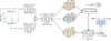 |
Fig. 2 Astromer’s multi-head attention mechanism. The light curve consists of magnitudes and timestamps (in MJDs). The magnitude values are processed through a FF neural network, while the timestamps of each observation are encoded using the positional encoder. The two representations are summed to form the input representation, which is then fed into the attention mechanism. This representation is projected into query (Q), key (K), and value (V) matrices using learned weight matrices. The attention mechanism computes attention weights (αi) using a softmax function applied to a scaled dot-product operation of the query and key vectors. The final multi-head attention output consists of multiple attention heads [h1, . . ., h#heads] concatenated and then transformed by a learned weight matrix. This transformed output is then used as the input representation for the next multi-head attention layer. |
2.2 Deep ensembles
Bayesian neural networks require significant computational resources, primarily due to the complex tuning necessary to achieve a consistent learning progress. In contrast, Lakshminarayanan et al. (2017) present DEs as a scalable and viable non-Bayesian alternative.
Consider a training dataset ![Mathematical equation: $\[\mathcal{D}=\left\{\left(\boldsymbol{x}_{i}, y_{i}\right)\right\}_{i=1}^{N}\]$](/articles/aa/full_html/2025/07/aa53388-24/aa53388-24-eq9.png) , where each xi ∈ ℝD is a D-dimensional feature vector. For a classification task, the labels yi are assumed to be one of K classes, i.e., yi ∈ {1, . . ., K}. Now, consider a predictive model (such as a neural network) that, for a given input x outputs a prediction
, where each xi ∈ ℝD is a D-dimensional feature vector. For a classification task, the labels yi are assumed to be one of K classes, i.e., yi ∈ {1, . . ., K}. Now, consider a predictive model (such as a neural network) that, for a given input x outputs a prediction ![Mathematical equation: $\[\hat{y}=f_{\theta}(\boldsymbol{x})\]$](/articles/aa/full_html/2025/07/aa53388-24/aa53388-24-eq10.png) , where θ are the parameters of the model. When estimating uncertainties for a new data point x*, we aim at modeling the predictive distribution as
, where θ are the parameters of the model. When estimating uncertainties for a new data point x*, we aim at modeling the predictive distribution as
![Mathematical equation: $\[p\left(y^* {\mid} \boldsymbol{x}^*, \mathcal{D}\right)=\int p\left(y^* {\mid} \boldsymbol{x}^*, \boldsymbol{\theta}\right) p(\boldsymbol{\theta} {\mid} \mathcal{D}) d \theta.\]$](/articles/aa/full_html/2025/07/aa53388-24/aa53388-24-eq11.png) (5)
(5)
This integral is often intractable and approximate inference is typically applied. Hence, one alternative for uncertainty estimation is the use of DEs. In our work, the strategy used involves training T independent neural network models, each with parameters ![Mathematical equation: $\[\left\{\boldsymbol{\theta}_{t}\right\}_{t=1}^{T}\]$](/articles/aa/full_html/2025/07/aa53388-24/aa53388-24-eq12.png) . The predictive outcome for a new test point x* is estimated by averaging the outputs from all T models:
. The predictive outcome for a new test point x* is estimated by averaging the outputs from all T models:
![Mathematical equation: $\[y^* \approx \frac{1}{T} \sum_{t=1}^T f_{\theta_t}\left(\boldsymbol{x}^*\right).\]$](/articles/aa/full_html/2025/07/aa53388-24/aa53388-24-eq13.png) (6)
(6)
Although this method is computationally intensive, it is easier to tune and can yield good performance while capturing predictive uncertainty.
We used DEs as the baseline uncertainty estimation technique, which uses the standard multi-head attention mechanism as shown in Fig. 3a. To calculate statistics over our uncertainty estimates, we trained ten ensembles, each consisting of ten deterministic models1. These models were independently trained with different random seeds, which are used to initialize model parameters to different starting values. Additionally, we trained each model with different training chunks of the complete dataset. This approach introduces variability in the learning process, promoting diverse model behaviors and mitigating overfitting, thereby enhancing the robustness of our UEs. The procedure was conducted for each survey.
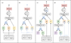 |
Fig. 3 Graphical representation of each method. For simplicity, each panel shows the first self-attention block, from the input representation (F F(x*) + P E(x*)) to the output of multi-head attention. Panel a shows the DEs approach, which relies on standard multi-head attention; attention scores αi are derived from the key (K) and query (Q) matrices (Eq. (2)), which are used to calculate the output hi (Eq. (4)). Panel b shows MC Dropout, which activates dropout both after the input and within the attention blocks (dashed blue lines). As a result, the query (Q), key (K) and value (V) matrices change with each forward pass. Panel c corresponds to the HSA approach, which introduces a hierarchical component, specifically, the key representation is redefined using a set of centroids (C) to produce a new key matrix ( |
![Mathematical equation: $\[\tilde{\boldsymbol{K}}\]$](/articles/aa/full_html/2025/07/aa53388-24/aa53388-24-eq14.png)
![Mathematical equation: $\[\tilde{\boldsymbol{\alpha}}_{i}, \hat{\boldsymbol{\alpha}}_{i}\]$](/articles/aa/full_html/2025/07/aa53388-24/aa53388-24-eq15.png)
2.3 Monte Carlo dropout
Dropout is a regularization technique used to prevent overfitting by deactivating neurons during the training stage (Srivastava et al. 2014). While initially aimed at mitigating overfitting, Gal & Ghahramani (2016) provided a theoretical framework for its application in uncertainty quantification. They demonstrated that MC Dropout works as an approximation of Bayesian inference in deep Gaussian processes. This is achieved by sampling neuron activations from a Bernoulli distribution across all hidden layers of the neural network during both training and inference stages.
MC Dropout uses dropout during inference to approximate the predictive distribution of Eq. (5). This adaptation allows MC Dropout to mimic an ensemble of diverse models. Each stochastic pass temporarily deactivates a random subset of neurons, and the expected value of the output y* for a given input x* is calculated by averaging the outputs from the model fθt(x*) over all samples, as shown in Eq. (6).
Consider the neural network layer i, which receives the output vector xi−1 from the preceding layer as its input. When dropout is applied with probability p, the output of layer i can be defined as
![Mathematical equation: $\[\boldsymbol{x}_i=\sigma\left(\boldsymbol{x}_{i-1} \mid \boldsymbol{W}_i, \boldsymbol{M}_i\right),\]$](/articles/aa/full_html/2025/07/aa53388-24/aa53388-24-eq16.png) (7)
(7)
where σ represents the activation function, Wi denotes the weights of layer i, and Mi are the variational parameters that modulate these weights during training and inference. The weights Wi are given by
![Mathematical equation: $\[\boldsymbol{W}_i=\boldsymbol{M}_i \cdot \operatorname{diag}\left(\left[z_{i, j}\right]_{j=1}^{K_i}\right), \qquad z_{i, j} \sim Bernoulli\left(1-p_i\right).\]$](/articles/aa/full_html/2025/07/aa53388-24/aa53388-24-eq17.png) (8)
(8)
Here zi,j = 0 indicates that the neuron j in layer i − 1 is dropped as an input to layer i.
This method offers advantages over DEs as it avoids the need to train multiple models while retaining the ability to estimate uncertainties by using the variability of subnetworks within a single model. The authors proposed applying this method to all hidden neural network layers. In adapting MC Dropout for transformers, following the methodology described by Shelmanov et al. (2021), we applied dropout to all layers in the model, including those within the attention blocks (see Fig. 3b). This strategy captures uncertainty at multiple levels of abstraction by introducing stochasticity throughout the entire network, ensuring that diverse model behaviors are accounted for, leading to more robust UEs than if dropout were applied only to the output layer.
2.4 Hierarchical stochastic attention
Pei et al. (2022) proposed HSA, an approach for producing probabilistic outputs rather than deterministic ones by injecting stochasticity through the Gumbel-softmax distribution (Jang et al. 2017). This uncertainty estimation method was applied to NLP tasks, achieving competitive predictive performance while allowing for uncertainty estimation. HSA is composed of two hierarchical stochastic self-attention mechanisms: stochasticity over the self-attention heads and over a set of learnable centroids.
As represented in Fig. 3c, stochastic self-attention replaces the traditional softmax activation function of the attention heads with the Gumbel-softmax distribution, which approximates samples from a categorical distribution with class probabilities θ = (θ1, θ2, . . ., θK) and associated logits values log(θi) (Jang et al. 2017; Huijben et al. 2022). The Gumbel-softmax distribution considers a temperature τ, and samples ![Mathematical equation: $\[\tilde{\boldsymbol{y}} \sim \mathcal{G}(\boldsymbol{\theta}, \tau)\]$](/articles/aa/full_html/2025/07/aa53388-24/aa53388-24-eq18.png) are computed as
are computed as
![Mathematical equation: $\[\tilde{y}_i=\frac{\exp \left(\left(\log \left(\theta_i\right)+g_i\right) / \tau\right)}{\sum_{j=1}^K \exp \left(\left(\log \left(\theta_j\right)+g_j\right) / \tau\right)},\]$](/articles/aa/full_html/2025/07/aa53388-24/aa53388-24-eq19.png) (9)
(9)
where gi represents independent and identically distributed (i.i.d.) samples from the Gumbel distribution, defined as gi = −log(−log(u)), where u is uniformly drawn from the interval [0, 1]. This approximation facilitates discrete choice sampling and gradient-based optimization needed on neural networks and that cannot be performed using a categorical distribution. Furthermore, using the temperature τ, the Gumbel-softmax distribution can be smoothly annealed into a categorical distribution: as τ → 0, the Gumbel-softmax samples are identical to the categorical distribution.
In stochastic self-attention, logits are computed as the logarithm of the dot product between the query and the key vectors, and the attention weights are calculated during a forward pass as follows:
![Mathematical equation: $\[\hat{\alpha}_{i, j}=\frac{\exp \left(\left(\log \left(\boldsymbol{q}_i^{\top} \boldsymbol{k}_j\right)+g_{i, j}\right) / \tau\right)}{\sum_{l=1}^L \exp \left(\left(\log \left(\boldsymbol{q}_i^{\top} \boldsymbol{k}_l^{\top}\right)+g_{i, l}\right) / \tau\right)},\]$](/articles/aa/full_html/2025/07/aa53388-24/aa53388-24-eq20.png) (10)
(10)
![Mathematical equation: $\[\hat{\boldsymbol{\alpha}}_i \sim \mathcal{G}\left(\boldsymbol{K} \boldsymbol{q}_i, \tau\right),\]$](/articles/aa/full_html/2025/07/aa53388-24/aa53388-24-eq21.png) (11)
(11)
where gi,j represents i.i.d. samples from the Gumbel distribution. Here, the Gumbel-softmax distribution plays a similar role as the traditional softmax, by normalizing scores across all keys k, but it allows one to sample from it and estimate gradients efficiently.
The second component of HSA forces heads to pay stochastic attention to a set of centroids. Instead of directly attending to each key, HSA employs the Gumbel-softmax distribution to group keys around c learnable centroids C ∈ ℝdk×c, where each centroid cj represents the j-th column of C and matches the dimension of each key head. The model starts by stochastically paying attention to the centroids, and then, a new set of keys ![Mathematical equation: $\[\left\{\tilde{\boldsymbol{k}}_{i}\right\}_{i=1}^{L}\]$](/articles/aa/full_html/2025/07/aa53388-24/aa53388-24-eq22.png) are calculated by weighting each centroid by this attention:
are calculated by weighting each centroid by this attention:
![Mathematical equation: $\[\tilde{\boldsymbol{\alpha}}_i \sim \mathcal{G}\left(\boldsymbol{C}^{\top} \boldsymbol{k}_i, \tau_1\right),\]$](/articles/aa/full_html/2025/07/aa53388-24/aa53388-24-eq23.png) (12)
(12)
![Mathematical equation: $\[\tilde{\boldsymbol{k}}_i=\sum_j \tilde{\alpha}_{i, j} \boldsymbol{c}_j.\]$](/articles/aa/full_html/2025/07/aa53388-24/aa53388-24-eq24.png) (13)
(13)
Here, gi,j are again sampled from the Gumbel-softmax distribution. The new keys of Eq. (13) were used to calculate the stochastic attention weights of Eq. (11), which were used to combine the values ![Mathematical equation: $\[\left\{\boldsymbol{v}_{i}\right\}_{i=1}^{L}\]$](/articles/aa/full_html/2025/07/aa53388-24/aa53388-24-eq25.png) as
as
![Mathematical equation: $\[\hat{\boldsymbol{\alpha}}_i \sim \mathcal{G}\left(\tilde{\boldsymbol{K}} \boldsymbol{q}_i, \tau_2\right),\]$](/articles/aa/full_html/2025/07/aa53388-24/aa53388-24-eq26.png) (14)
(14)
![Mathematical equation: $\[\boldsymbol{h}_i=\sum_{j=1}^L \hat{\alpha}_{i, j} \boldsymbol{v}_j,\]$](/articles/aa/full_html/2025/07/aa53388-24/aa53388-24-eq27.png) (15)
(15)
where ![Mathematical equation: $\[\tilde{\boldsymbol{k}}_{i}\]$](/articles/aa/full_html/2025/07/aa53388-24/aa53388-24-eq28.png) is represented as the i-th row of matrix
is represented as the i-th row of matrix ![Mathematical equation: $\[\tilde{\boldsymbol{K}} \in \mathbb{R}^{L \times d_{k}}\]$](/articles/aa/full_html/2025/07/aa53388-24/aa53388-24-eq29.png) .
.
Notice the hierarchical nature of HSA: the method employs the Gumbel-softmax distribution twice; initially to generate the new keys ![Mathematical equation: $\[\left\{\tilde{\boldsymbol{k}}_{i}\right\}_{i=1}^{L}\]$](/articles/aa/full_html/2025/07/aa53388-24/aa53388-24-eq30.png) , and a second time to compute the outputs for each attention block
, and a second time to compute the outputs for each attention block ![Mathematical equation: $\[\left\{\boldsymbol{h}_{i}\right\}_{i=1}^{L}\]$](/articles/aa/full_html/2025/07/aa53388-24/aa53388-24-eq31.png) .
.
We implemented the HSA approach in the Astromer attention mechanism, which captures predictive uncertainties through multiple forward passes during the inference stage, similar to the MC Dropout approach. We further discuss how the temperature of the Gumbel-softmax distributions affects the amount of stochasticity introduced into the model and its impact on uncertainty estimation.
2.5 Hierarchical attention with Monte Carlo dropout
We propose a combination of MC Dropout and the hierarchical attention strategy for quantifying uncertainty in Astromer. This approach incorporates learnable centroids ci in the attention blocks without applying the Gumbel-softmax distribution, but instead adding MC Dropout to the attention blocks. This allows us to achieve a regularization effect through the key head’s attention to the centroids, while adding stochasticity without the use of the Gumbel-softmax distribution. The approach is defined as follows:
![Mathematical equation: $\[\tilde{\boldsymbol{\alpha}}_i=\operatorname{softmax}\left(\frac{\boldsymbol{C}^{\mathrm{T}} \boldsymbol{k}_i}{\sqrt{d_k}}\right),\]$](/articles/aa/full_html/2025/07/aa53388-24/aa53388-24-eq32.png) (16)
(16)
![Mathematical equation: $\[\tilde{\boldsymbol{k}}_i=\sum_j \tilde{\alpha}_{i, j} \boldsymbol{c}_j,\]$](/articles/aa/full_html/2025/07/aa53388-24/aa53388-24-eq33.png) (17)
(17)
where dk is the original scaling factor, and C is the matrix with the centroids as columns from Eq. (13). The final attention weights are then computed using
![Mathematical equation: $\[\hat{\boldsymbol{\alpha}}_i=\operatorname{softmax}\left(\frac{\tilde{\boldsymbol{K}} \boldsymbol{q}_i}{\sqrt{d_k}}\right),\]$](/articles/aa/full_html/2025/07/aa53388-24/aa53388-24-eq34.png) (18)
(18)
![Mathematical equation: $\[\boldsymbol{h}_i=\sum_j \hat{\alpha}_{i, j} \boldsymbol{v}_j,\]$](/articles/aa/full_html/2025/07/aa53388-24/aa53388-24-eq35.png) (19)
(19)
In this context, stochasticity is introduced by activating the dropout layers within each attention block during the inference stage. Figure 3d provides a graphical representation of this approach.
2.6 Uncertainty estimates
When a model is trained using only a maximum likelihood approach, the softmax activation function is prone to generate overconfident predictions (Guo et al. 2017). To explore and quantify the uncertainty inherent in our model’s predictions, we employed UEs. These estimates are not intended to assess the quality of uncertainty quantification, but rather to measure the extent and variability of the uncertainty itself. While UEs capture the extent and variability of uncertainty, their quality must be assessed separately to determine how well they reflect true predictive uncertainty, as discussed in Sect. 2.7
Uncertainty in classification arises from multiple sources, including inherent noise in the data (aleatoric uncertainty) and uncertainty caused by a lack of knowledge (epistemic uncertainty), for example, in the model parameters. To fully characterize these uncertainties and make informed decisions, it is essential to employ multiple UEs, each capturing different aspects of predictive confidence and model reliability.
For the MC Dropout model variants, each UE is calculated by conducting T forward pass inference runs with dropout activated. In the case of HSA, the variation in the T inference runs is obtained through samples drawn from the Gumbel-softmax distribution. For the DEs baseline, T corresponds to the number of independent models. Using these T inference runs, we calculated the following UEs:
-
Sampled maximum probability (SMP):
![Mathematical equation: $\[1-\max _{c \in C} \bar{p}(y=c {\mid} x),\]$](/articles/aa/full_html/2025/07/aa53388-24/aa53388-24-eq36.png) (20)
(20)where
![Mathematical equation: $\[\bar{p}(y=c \mid x)=\frac{1}{T} \sum_{t=1}^{T} p_{t}(y=c \mid x)\]$](/articles/aa/full_html/2025/07/aa53388-24/aa53388-24-eq37.png) is the average probability of each class c across T forward passes for a given input x (with pt(y = c|x) being the probability of class c at the t-th forward pass inference run). The SMP provides an intuitive measure of confidence by considering the maximum mean predicted probability across classes. If a model is highly confident in a prediction across different stochastic samples, the maximum average probability will be high, indicating low total uncertainty.
is the average probability of each class c across T forward passes for a given input x (with pt(y = c|x) being the probability of class c at the t-th forward pass inference run). The SMP provides an intuitive measure of confidence by considering the maximum mean predicted probability across classes. If a model is highly confident in a prediction across different stochastic samples, the maximum average probability will be high, indicating low total uncertainty. -
Probability variance (PV); Gal et al. 2017):
![Mathematical equation: $\[\frac{1}{C} \sum_{c=1}^C\left(\frac{1}{T} \sum_{t=1}^T\left(p_t(y=c \mid x)-\bar{p}(y=c \mid x)\right)^2\right).\]$](/articles/aa/full_html/2025/07/aa53388-24/aa53388-24-eq38.png) (21)
(21)This is the variance averaged over all C classes. PV assesses how consistently the model predicts the same class probabilities across different inference runs, providing an insight into the predictive stability. If a model is uncertain about a sample, different stochastic passes will produce varying probabilities, leading to high variance. Low variance indicates a confident model. PV captures epistemic uncertainty, as it quantifies how much the model’s predictions fluctuate due to weight uncertainty, but, to some extent it also captures aleatoric uncertainty. For example, in cases of high aleatoric uncertainty (e.g., ambiguous samples, overlapping class distributions, or noisy measurements), the model’s probability estimates can vary across stochastic passes even if the model parameters are fully known.
-
Bayesian active learning by disagreement (BALD; Houlsby et al. 2011):
![Mathematical equation: $\[-\sum_{c=1}^C \overline{p^c} \log \left(\overline{p^c}\right)+\frac{1}{T} \sum_{t=1}^T \sum_{c=1}^C p_t^c ~\log \left(p_t^c\right),\]$](/articles/aa/full_html/2025/07/aa53388-24/aa53388-24-eq39.png) (22)
(22)where
![Mathematical equation: $\[\overline{p^{c}}=\bar{p}(y=c \mid x)\]$](/articles/aa/full_html/2025/07/aa53388-24/aa53388-24-eq40.png) , and
, and ![Mathematical equation: $\[p_{t}^{c}=p_{t}(y=c \mid x)\]$](/articles/aa/full_html/2025/07/aa53388-24/aa53388-24-eq41.png) . The first term is the entropy of the average predictions across the ensemble of models, whereas the second term calculates the mean entropy of individual predictions from each model within the ensemble, reflecting the average uncertainty inherent in each model’s predictions. BALD captures epistemic uncertainty: the first term of Eq. (22) corresponds to the uncertainty (as defined by the entropy) of the final averaged prediction, i.e., the total uncertainty, while the second term corresponds to the average entropy over different stochastic passes, i.e., the aleatoric uncertainty. By subtracting them, BALD represents the epistemic uncertainty. Unlike PV, BALD directly quantifies the uncertainty about the model’s parameters rather than just the spread of probability estimates.
. The first term is the entropy of the average predictions across the ensemble of models, whereas the second term calculates the mean entropy of individual predictions from each model within the ensemble, reflecting the average uncertainty inherent in each model’s predictions. BALD captures epistemic uncertainty: the first term of Eq. (22) corresponds to the uncertainty (as defined by the entropy) of the final averaged prediction, i.e., the total uncertainty, while the second term corresponds to the average entropy over different stochastic passes, i.e., the aleatoric uncertainty. By subtracting them, BALD represents the epistemic uncertainty. Unlike PV, BALD directly quantifies the uncertainty about the model’s parameters rather than just the spread of probability estimates.
Each of these UEs are different ways of quantifying uncertainty from probabilistic models. Their conceptual differences lie in what aspect of uncertainty they capture and how they use multiple stochastic forward passes.
2.7 Evaluating uncertainty estimation via misclassification detection
A well-calibrated uncertainty estimation model should exhibit high uncertainty for incorrect predictions while maintaining low uncertainty for correct ones. To evaluate the performance of uncertainty estimation, we defined a misclassification detection task. Although all of our models were trained as multi-class classifiers, we reformulated the evaluation during the testing phase as a binary classification problem focused on identifying misclassifications. This approach is aligned with the work done by Shelmanov et al. (2021) and Vazhentsev et al. (2022) for the NLP tasks.
Specifically, we constructed new binary instances ![Mathematical equation: $\[\tilde{e}_{i}\]$](/articles/aa/full_html/2025/07/aa53388-24/aa53388-24-eq42.png) as follows:
as follows:
![Mathematical equation: $\[\tilde{e}_i= \begin{cases}1, & y_i \neq \hat{y}_i, \\ 0, & y_i=\hat{y}_i,\end{cases}\]$](/articles/aa/full_html/2025/07/aa53388-24/aa53388-24-eq43.png) (23)
(23)
where yi is the true label, and ![Mathematical equation: $\[\hat{y}_{i}\]$](/articles/aa/full_html/2025/07/aa53388-24/aa53388-24-eq44.png) is the original predicted label. The new instances
is the original predicted label. The new instances ![Mathematical equation: $\[\tilde{e}_{i}\]$](/articles/aa/full_html/2025/07/aa53388-24/aa53388-24-eq45.png) indicate whether the model made a mistake in predicting the label of the variable source.
indicate whether the model made a mistake in predicting the label of the variable source.
To measure the quality of UE, we computed the receiver operating characteristic (ROC) area under the curve (AUC) scores based on the binary labels ![Mathematical equation: $\[\tilde{e}_{i}\]$](/articles/aa/full_html/2025/07/aa53388-24/aa53388-24-eq46.png) and their corresponding UE scores. We used the UE values as discrimination values to build the ROC curve, which plots the true positive rate (TPR) against the false positive rate (FPR) across various thresholds (Swets 1988). For a specific UE threshold, the TPR and FPR are calculated as
and their corresponding UE scores. We used the UE values as discrimination values to build the ROC curve, which plots the true positive rate (TPR) against the false positive rate (FPR) across various thresholds (Swets 1988). For a specific UE threshold, the TPR and FPR are calculated as
![Mathematical equation: $\[\mathrm{TPR}=\frac{\mathrm{TP}}{\mathrm{TP}+\mathrm{FN}},\]$](/articles/aa/full_html/2025/07/aa53388-24/aa53388-24-eq47.png)
and
![Mathematical equation: $\[\mathrm{FPR}=\frac{\mathrm{FP}}{\mathrm{FP}+\mathrm{TN}},\]$](/articles/aa/full_html/2025/07/aa53388-24/aa53388-24-eq48.png)
where
TP is the number of instances that have an UE higher than the threshold, and
![Mathematical equation: $\[\tilde{e}_{i}\]$](/articles/aa/full_html/2025/07/aa53388-24/aa53388-24-eq49.png) = 1 (misclassified instances with high uncertainty),
= 1 (misclassified instances with high uncertainty),TN is the number of instances that have an UE lower than the threshold, and
![Mathematical equation: $\[\tilde{e}_{i}\]$](/articles/aa/full_html/2025/07/aa53388-24/aa53388-24-eq50.png) = 0 (correctly classified instances with low uncertainty),
= 0 (correctly classified instances with low uncertainty),FP is the number of instances that have an UE higher than the threshold, and
![Mathematical equation: $\[\tilde{e}_{i}\]$](/articles/aa/full_html/2025/07/aa53388-24/aa53388-24-eq51.png) = 0 (correctly classified instances with high uncertainty),
= 0 (correctly classified instances with high uncertainty),FN is the number of instances that have an UE lower than the threshold, and
![Mathematical equation: $\[\tilde{e}_{i}\]$](/articles/aa/full_html/2025/07/aa53388-24/aa53388-24-eq52.png) = 1 (misclassified instances with low uncertainty).
= 1 (misclassified instances with low uncertainty).
We evaluated statistical significance of our results using the Wilcoxon-Mann Whitney (WMW) test. The WMW test, a nonparametric alternative to the t-test, evaluates data based on ranks rather than assuming normality or equal variances. This test ranks all observations from two independent samples, X and Y, and calculates the test statistic, U, using the ranks from the smaller sample. The null hypothesis states that X and Y have identical distributions. Significant deviations in U suggests differing distributions, with statistical significance indicating disparities in central tendencies (Fay & Proschan 2010; Pett 2015).
3 Experimental setup
In this section, we detail our experimental setup, where we evaluate the models using three labeled astronomical catalogs. We balanced the number of samples per class in small chunks for both the training and testing stages. The experiments were conducted on an Nvidia RTX A5000 GPU, our focus was on detecting misclassifications by converting the multi-class task into a binary problem, thus providing a clear understanding of model performance under varied data scenarios.
We compared the performance of baseline and the proposed models on three labeled catalogs of variable stars: the Optical Gravitational Lensing Experiment (OGLE-III; Udalski 2003), the Asteroid Terrestrial-impact Last Alert System (ATLAS; Heinze et al. 2018), and the MACHO dataset. We considered the classification scheme and filtering methods previously selected by Becker et al. (2020) and used by Donoso-Oliva et al. (2023), as detailed in Table 1. These catalogs contain light curves observed through different spectral filters, offering a broad spectrum of data for analysis.
Preserving in-domain integrity during model testing was crucial to our methodology. This principle required evaluating models on data with distributional characteristics similar to those of the training set. Therefore, we avoided combining the test sets from the three catalogs during inference, despite some catalogs sharing classes. This approach highlights the importance of testing models in conditions that mirror their training environment. Although the OGLE-III and MACHO datasets share similar wavelength ranges, the distinct spectral band of the ATLAS catalog indicates the need for a meticulous in-domain evaluation approach.
To emulate scenarios with a small amount of data, we selected 500 samples per class for training and 100 samples per class for test sets from the raw data (see Table 2). A validation set was created by randomly selecting 30% of the training set.
We used ten ensembles for the baseline and ten variants models per approach. A single test set per survey was used to compare the performance of the models. Consequently, we collected ten predictions for each approach, which enabled us to calculate the mean and standard deviation of the samples and thereby conduct significance testing.
For the optimization technique, we chose Adam (Kingma & Ba 2015) with a learning rate of 10−3. The batch size was of 512, and as a regularization technique, we used early stopping with a patience of 20 epochs on the validation loss. We used the same hyperparameter settings for each experiment.
Variable star classes of each survey associated with the corresponding tag.
Data distribution in terms of the number of light curves.
4 Results
4.1 Predictive performance
We evaluated the predictive performance using the macro-average of multiclass classification metrics over the three single-band datasets: MACHO, ATLAS, and OGLE-III. Table 3 presents the test sets F1 score, accuracy and precision of the HSA, MC Dropout, HA-MC Dropout, and DEs methods.
The DEs baseline serves as a consistent benchmark, achieving macro F1 scores of 68.6, 77.8, and 67.3 on MACHO, ATLAS, and OGLE-III, respectively. The MC Dropout method demonstrates a marginal performance improvement on the ATLAS test set, with a similar macro F1-score and accuracy of 78.8%, indicating limited gains over the baseline.
In contrast, the HSA method significantly improves performance across all datasets, even when tested on datasets with varying numbers of classes (six classes in MACHO, four in ATLAS, and ten in OGLE-III). This demonstrates its ability to perform well across varying levels of class complexity, reflecting its capacity to capture more intricate patterns. However, it exhibits more variability in terms of standard deviation compared to other approaches, with the variability in performance metrics close to 2%. This increased variability may be attributable to the stochasticity introduced by the Gumbel-softmax distribution, which can impact the predictive performance consistency across different runs. Consequently, while HSA improves the overall performance, its stability across different runs can be less consistent than that of other approaches.
The proposed HA-MC Dropout significantly outperforms the other methods achieving higher scores across all metrics. HA-MC Dropout achieves macro F1-scores of 76.6, 84.0, and 79.8 on MACHO, ATLAS, and OGLE-III, respectively, marking a substantial improvement in multi-class classification performance. Particularly in the dataset with 10 classes, OGLE-III, HA-MC Dropout obtained a more than 10% improvement compared to the baseline, with an F1-score, accuracy, and precision of 79.8, 80.5, and 80.0. These results indicate that the integration of hierarchical attention mechanisms with MC Dropout not only enhances predictive accuracy but also provides a more reliable model with reduced variance in performance metrics. This can be explained by the way stochasticity is injected into the model: unlike HSA that relies on the Gumbel-softmax distribution, HA-MC Dropout activates dropout during the inference stage to estimate uncertainty.
To summarize, two of the methods, HSA and HA-MC Dropout, surpass the DEs baseline. This indicates that combining hierarchical attention with a stochastic component yields improvements in multi-class classification tasks. The comparison presented in Table 3 represents the first stage of our analysis, focusing on the multi-class evaluation to establish a general understanding of the performance enhancements provided by these methods. However, the interpretability and trustworthiness of the results are further supported by the uncertainty estimation, which provides insights into the reliability of our classification outcomes. We extend our analysis by considering the impact of uncertainty estimation on the misclassification task in Sect. 4.2, providing a more comprehensive evaluation of the robustness and reliability of the different methods in handling complex classification tasks.
Macro average multi-class metrics scores (%) on MACHO, ATLAS, and OGLE-III test sets.
4.2 Predictive uncertainty
We evaluated the methods in terms of the predictive uncertainty using the misclassification detection task, as described in Sect. 2.7, on the MACHO, ATLAS, and OGLE-III test sets. Table 4 shows the ROC AUC scores for the different UEs. In this context, the ideal classifier is one that aligns UEs with the misclassification task: misclassified instances should be associated with high uncertainty, while correctly classified instances should correspond to low uncertainty.
We compared the baseline DE method against MC Dropout, HSA, and HA-MC Dropout. The evaluation metric used is the absolute ROC AUC score, which quantifies the ability of the model to discern between misclassifications and correct classifications by using the UEs as discrimination scores. The UEs used to calculate each ROC AUC are SMP, PV, and BALD. Specifically, for the baseline, the mean absolute ROC AUC is presented, whereas for the other methods, we report the performance differences relative to the baseline’s corresponding UEs, highlighting any statistically significant improvements (p-values ≤0.05). Note that the results are grouped by dataset.
Standard deviations are reported to reflect the variability across ten model iterations. For the baseline, this includes results from ten independent ensemble runs, where each run consists of ten separately trained deterministic models. For MC Dropout, HSA, and HA-MC Dropout, the results are based on ten independently trained models, with T = 10 stochastic inference runs performed per object for each model.
The DEs consistently achieve an average ROC AUC exceeding 70% across all UEs and datasets. This performance highlights their capability to identify potential errors through probabilistic outputs. MC Dropout excels in capturing predictive uncertainty when using PV and BALD scores for ROC AUC calculation, surpassing the baseline in misclassification detection tasks across all datasets. This is especially noticeable on the OGLE-III dataset, where the incremental percentage differences in ROC AUC relative to the baseline are 4.3 ± 1.6% and 4.2 ± 1.6%, respectively.
Conversely, HSA registers significant improvements with PV and BALD on the ATLAS and OGLE-III datasets. However, it fails to demonstrate an enhancement on the MACHO test set with any of the UEs provided. In the case of SMP scores, noticeable differences between the baseline arise where negative values indicate a reduction relative to the baseline.
To address these challenges, we introduced the HA-MC Dropout method, which, as aforementioned, combines the strengths of MC Dropout and HSA. This hybrid approach significantly outperforms both individual methods, especially in SMP scores, where it rivals or even surpasses the baseline. For instance, it achieves an improvement of 2.1 ± 1.2% on MACHO. The most substantial improvements are observed with PV on OGLE-III, where it reaches 8.5 ± 1.6%, doubling the improvement achieved by MC Dropout. Additionally, with PV, the improvement on MACHO is 2.5 ± 2.3%, and using BALD yields 3.8 ± 2.4% on ATLAS. Consequently, HA-MC Dropout not only mitigates the limitations of its constituent methods but also establishes a new benchmark for balancing predictive accuracy and uncertainty quantification across diverse datasets.
To further assess the impact of centroids, we removed them from the combination of the Gumbel-softmax and centroids in HSA. For this, we created a version of the model that directly introduces stochasticity in the self-attention heads through a Gumbel-softmax distribution. This resulted in a deterioration of uncertainty quantification performance compared to the other models, as explained in Appendix A.
UEs in the misclassification task on the MACHO, ATLAS, and OGLE-III test sets.
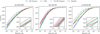 |
Fig. 4 Accuracy-rejection curves for the MACHO (a), ATLAS (b), and OGLE-III (c) datasets. The techniques compared are MC Dropout (dash-squared line), HSA (dash-triangular line), HA-MC Dropout (dash-dotted line), and the baseline model (solid line). Insets zoom into the lower rejection rate region (0–0.3) to emphasize differences at low rejection levels. |
4.3 Accuracy-rejection plots
We present a practical application of our misclassification framework by using the accuracy-rejection plots (Nadeem et al. 2009) for MACHO, ATLAS, and OGLE-III test sets, as illustrated in Figs. 4a, b, and c. These plots emulate a scenario reflecting a hybrid machine-human behavior, wherein the machine abstains from classifying the most uncertain samples. This approach allows us to visualize accuracy as a function of the rejection rate. In all figures, confidence levels were assessed using the PV score, and the shaded areas represent the standard deviation across ten iterations of each approach. Additionally, each plot includes a zoomed inset focusing on the rejection rate interval from 0.1 to 0.3, providing a detailed comparison of the various methods within this specific range.
As a guideline, in Fig. 4a, the accuracy-rejection plot for the MACHO test set suggests that maintaining an accuracy threshold above 80% requires a rejection rate of ~0.15 for MC Dropout and ~0.1 for the DEs baseline and HSA. HA-MC Dropout is able to keep an 80% accuracy by rejecting fewer than the ~5% most uncertain predicted labels in the MACHO dataset.
Notably, the HA-MC Dropout method surpasses both the baseline and other techniques for every rejection rate, highlighting its potential. Although HSA shows a marginally higher mean accuracy compared to the baseline, the baseline demonstrates lower variability at a rejection rate of 0.2, indicating higher consistency. Meanwhile, MC Dropout aligns closely with the baseline performance until a rejection rate of ~0.4.
Figure 4b presents the accuracy-rejection plot for the ATLAS test set. Below a rejection rate of ~0.2, HA-MC Dropout shows a performance comparable to the baseline. However, at a rejection rate of ~0.2, the HA-MC Dropout method achieves a mean accuracy of approximately 0.93, surpassing the baseline by about 0.02 points, demonstrating its superior performance.
Finally, Fig. 4c details the accuracy-rejection scenario for the OGLE-III dataset, indicating that both HA-MC Dropout and HSA outperform the baseline, with HA-MC Dropout needing a 20% rejection rate to achieve a mean accuracy score of 0.90. HSA follows closely with an accuracy of 0.87, while the baseline achieves 0.84 and MC Dropout 0.82. This scenario underscores the necessity for expert intervention to maintain high accuracy levels, demonstrating that HA-MC Dropout achieves superior results with minimal expert involvement.
The differences observed in the accuracy-rejection curves for the different datasets stem from dataset-specific characteristics such as noise levels, sampling cadence, and the specific types of variable stars included. OGLE-III, for instance, contains ten classes, making classification inherently more challenging than ATLAS (four classes) and MACHO (six classes). This variability impacts how uncertainty is distributed among predictions, leading to differences in the accuracy-rejection curves.
The analysis of these plots presents that, across all datasets evaluated, the performance curves of the MC Dropout approach align with the baseline model for a rejection rate higher than ~0.4. This consistency at a specified threshold highlights the capability of the MC Dropout to maintain accuracy while also providing estimates of uncertainty. Conversely, the HA-MC Dropout method is a better option to other methods in all datasets. Despite the baseline showing a lower standard deviation in the OGLE and MACHO datasets, the overall accuracy score consistency across different astronomical datasets highlights the resilience of HA-MC Dropout. This robust performance affirms the cost-efficiency of implementing HA-MC Dropout for estimating uncertainty on transformer-based classifiers, making them well suited for real-world applications.
5 Discussion and conclusions
We have investigated the application of uncertainty estimation techniques to enhance the reliability and interpretability of transformer-based models for light-curve classification in the context of variable star analysis. By implementing and evaluating DEs, MC Dropout, HSA, and our proposed hybrid method, HA-MC Dropout, in Astromer, we have demonstrated the potential of these techniques in capturing predictive uncertainty and improving misclassification detection.
Our empirical results highlight that HA-MC Dropout consistently outperforms other methods in terms of predictive accuracy and uncertainty estimation across various datasets. This suggests that integrating hierarchical attention mechanisms with MC Dropout offers a powerful approach to enhancing the robustness and reliability of transformer-based models in complex classification tasks. The superior performance of HA-MC Dropout, particularly in scenarios with limited data, highlights its potential for real-world applications in scenarios with limited data and class distribution challenges.
The accuracy-rejection plots provide valuable insights into the practical implications of our work. These plots demonstrate that HA-MC Dropout enables the model to achieve higher accuracy levels with fewer rejected samples, showcasing its potential for automating the classification process while maintaining high confidence in the results. The consistent performance of MC Dropout across different datasets further reinforces its value as a viable alternative to the other approaches. Hence, it offers a computationally efficient and effective method for uncertainty estimation in transformer-based models.
A crucial aspect of our framework is that we evaluated model performance based not only on predictive metrics, such as the macro F1-score, accuracy, and precision, but also on its ability to generate meaningful predictive uncertainty. Our results demonstrate that uncertainty models should not be judged solely on a single estimator but rather through a comprehensive evaluation that considers multiple UEs. Specifically, HA-MC Dropout notably improves uncertainty estimation when using PV and BALD (epistemic uncertainty), achieving statistically significant improvements (p-value ≤0.05) over the baseline. At the same time, HA-MC Dropout yields statistically similar results to the baseline in terms of the quality of the estimated total uncertainty for MACHO and ATLAS, as measured by the SMP, highlighting the importance of adopting a broader perspective when estimating uncertainty scores.
An important consideration when comparing the classification performance stability of different models is the extent of stochasticity they introduce. Table 3 shows that although the architectures of HA-MC Dropout and HSA are similar, HA-MC Dropout shows a lower variance in classification performance than HSA. At the same time, the quality of the epistemic uncertainty estimation of HA-MC Dropout, as shown in Table 4, is better than that of HSA, as indicated by lower ROC AUC values when using BALD. This suggests that classification performance stability is closely linked to the quality of uncertainty estimation.2 The same interpretation can be made when comparing the DEs baseline with MC Dropout, which share the same main architecture. This suggests that the increased variance in F1-scores observed in less stable models is a consequence of their inability to produce reliable uncertainty estimations. Although directly quantifying the level of injected stochasticity remains a challenge, our findings indicate that the quality of uncertainty estimation plays a key role in model stability.
The findings of this study have significant implications for the future of variable star classification, particularly in the era of next-generation large-scale astronomical surveys such as the LSST. The ability to quantify uncertainty and detect misclassifications will be crucial to ensuring the reliability and interpretability of automated classification systems. The work presented here offers a promising step toward achieving this goal, paving the way for a more robust and trustworthy analysis of astronomical light curves.
Future research directions include an exploration of the application of our work to multiband light-curve models (e.g., Cabrera-Vives et al. 2024). Additionally, considering the impact of different data preprocessing and augmentation strategies on uncertainty estimation could provide valuable insights that could be used to help improve the performance of the transformer-based model in challenging scenarios. Human feedback for objects classified by the model with low certainty can also be added into a human-in-the-loop framework (see, e.g., Richards et al. 2011; Masci et al. 2014; Martínez-Palomera et al. 2018; Ishida et al. 2019; Kennamer et al. 2020; Leoni et al. 2022).
In summary, HA-MC Dropout has proven to be competitive against the DEs baseline in three astronomical datasets with different variable star taxonomies. Transformer-based models have established their status as the state-of-the-art models across various fields. We emphasize the significance of developing reliable models that can reduce computational expenses when being trained: DEs need to train multiple models, while the MC Dropout strategy uses a single trained model. We believe that the capacity to accurately assess uncertainty can economize human labor while also improving confidence in the conclusions derived from these models.
Acknowledgements
The authors acknowledge support from the National Agency for Research and Development (ANID) grants: FONDECYT regular 1231877 (MCL, GCV, DMC, CDO); Millennium Science Initiative Program – NCN2021_080 (GCV, CDO) and ICN12_009 (GCV, CDO).
Appendix A Gumbel-softmax over self-attention heads
We explored an alternative design for HSA by injecting stochasticity into the attention heads without incorporating the hierarchical component, sampling the attention scores from a Gumbel-softmax distribution (Pei et al. 2022). We assessed the impact of this modification by computing the macro F1-score across the MACHO, ATLAS, and OGLE-III test sets, obtaining 69.0 ± 1.8, 78.2 ± 2.0, and 67.4 ± 3.8 respectively. These results closely mirror those obtained using MC Dropout in Table 3, suggesting that Gumbel-softmax stochastic attention does not significantly enhance the multi-class classification performance. A detailed evaluation, presented in Table A.1, further indicates that Stochastic Attention underperforms relative to the baseline and does not consistently improve misclassification UEs. The detailed results underscore the limited efficacy of the Gumbel-softmax approach in this context, suggesting that retaining dropout mechanisms leads to better performance improvements.
Comparison of UEs in the misclassification task on the MACHO, ATLAS, and OGLE-III test sets for stochastic attention and the DEs method.
Appendix B Effect of temperature on hierarchical stochastic attention
In the architecture of HSA, we used the Gumbel-softmax distribution twice within the attention mechanism: first, during the centroidbased computation of the new keys (see Eq. 13), where we refer to the temperature as τ1; and second, in the interaction with the query vector (see Eq. 15), where we denote the temperature as τ2. In this work we used τ1 = 8 and τ2 = 30. The temperature hyperparameter in the Gumbel-softmax distribution controls the smoothness of the sampling process: lower values lead to more discrete (one-hot-like) samples, while higher values produce smoother, more uniform distributions (Jang et al. 2017). To investigate the impact of the temperature hyperparameters on the performance of HSA, we conducted a series of experiments varying the values of τ1 and τ2 from 0.25 to 32, increasing in powers of two.
Figure B.1 shows how the distribution of F1-scores changes under different temperature values: the left panel shows the mean F1-scores over ten samples for each object in the MACHO test set, while the right panel shows their standard deviation. The region where τ1 ≥ 2 and τ2 ≥ 4 yields stable results with a mean F1-score around 0.74 and a standard deviation around 0.2. Consistent with the results of Jang et al. (2017), we also observe that lower temperature values are associated with an increased variance in performance. These results imply that, for the temperature values used in our work (τ1 = 8 and τ2 = 30) the uncertainty estimation of HSA cannot be further improved by tuning the level of injected stochasticity through the Gumbel-softmax.
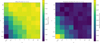 |
Fig. B.1 Effect of Gumbel-softmax temperatures on HSA performance. We show heatmaps of the mean F1-score (left) and standard deviation (right) over multiple runs on the MACHO test set for different combinations of the Gumbel-softmax temperature parameters, τ1 and τ2. Warmer colors in the left panel indicate higher mean F1-scores, while cooler colors in the right panel reflect a lower variance. |
References
- Alcock, C., Allsman, R., Alves, D. R., et al. 2000, ApJ, 542, 281 [NASA ADS] [CrossRef] [Google Scholar]
- Bassi, S., Sharma, K., & Gomekar, A. 2021, Front. Astron. Space Sci., 8, 718139 [Google Scholar]
- Becker, I., Pichara, K., Catelan, M., et al. 2020, MNRAS, 493, 2981 [NASA ADS] [CrossRef] [Google Scholar]
- Blundell, C., Cornebise, J., Kavukcuoglu, K., & Wierstra, D. 2015, in International Conference on Machine Learning, PMLR, 1613 [Google Scholar]
- Cabrera-Vives, G., Reyes, I., Förster, F., Estévez, P. A., & Maureira, J.-C. 2016, in 2016 International Joint Conference on Neural Networks (IJCNN), 251 [CrossRef] [Google Scholar]
- Cabrera-Vives, G., Moreno-Cartagena, D., Astorga, N., et al. 2024, A&A, 689, A289 [NASA ADS] [CrossRef] [EDP Sciences] [Google Scholar]
- Carrasco-Davis, R., Cabrera-Vives, G., Förster, F., et al. 2019, PASP, 131, 108006 [NASA ADS] [CrossRef] [Google Scholar]
- Ciucă, I., Kawata, D., Miglio, A., Davies, G. R., & Grand, R. J. 2021, MNRAS, 503, 2814 [Google Scholar]
- Devlin, J., Chang, M.-W., & Lee, K. 2019, in Proceedings of NAACL-HLT, 4171 [Google Scholar]
- Donoso-Oliva, C., Cabrera-Vives, G., Protopapas, P., Carrasco-Davis, R., & Estévez, P. A. 2021, MNRAS, 505, 6069 [CrossRef] [Google Scholar]
- Donoso-Oliva, C., Becker, I., Protopapas, P., et al. 2023, A&A, 670, A54 [NASA ADS] [CrossRef] [EDP Sciences] [Google Scholar]
- Fay, M. P., & Proschan, M. A. 2010, Statist. Surv., 4, 1 [Google Scholar]
- Feast, M. W., Menzies, J. W., Matsunaga, N., & Whitelock, P. A. 2014, Nature, 509, 342 [Google Scholar]
- Gal, Y., & Ghahramani, Z. 2016, in International Conference on Machine Learning, PMLR, 1050 [Google Scholar]
- Gal, Y., Islam, R., & Ghahramani, Z. 2017, in International Conference on Machine Learning, PMLR, 1183 [Google Scholar]
- Ganaie, M. A., Hu, M., Malik, A., Tanveer, M., & Suganthan, P. 2022, Eng. Appl. Artif. Intell., 115, 105151 [CrossRef] [Google Scholar]
- Gawlikowski, J., Tassi, C. R. N., Ali, M., et al. 2023, Artif. Intell. Rev., 56, 1513 [Google Scholar]
- Guo, C., Pleiss, G., Sun, Y., & Weinberger, K. Q. 2017, in International Conference on Machine Learning, PMLR, 1321 [Google Scholar]
- Heinze, A., Tonry, J. L., Denneau, L., et al. 2018, AJ, 156, 241 [NASA ADS] [CrossRef] [Google Scholar]
- Hochreiter, S., & Schmidhuber, J. 1997, Neural Computat., 9, 1735 [Google Scholar]
- Houlsby, N., Huszár, F., Ghahramani, Z., & Lengyel, M. 2011, arXiv e-prints [arXiv:1112.5745] [Google Scholar]
- Huijben, I. A., Kool, W., Paulus, M. B., & Van Sloun, R. J. 2022, IEEE Trans. Pattern Anal. Mach. Intell., 45, 1353 [Google Scholar]
- Ishida, E., Beck, R., González-Gaitán, S., et al. 2019, MNRAS, 483, 2 [NASA ADS] [CrossRef] [Google Scholar]
- Ivezić, Ž., Kahn, S. M., Tyson, J. A., et al. 2019, ApJ, 873, 111 [Google Scholar]
- Jang, E., Gu, S., & Poole, B. 2017, in 5th International Conference on Learning Representations, ICLR 2017, Toulon, France, April 24–26, 2017, Conference Track Proceedings (OpenReview.net) [Google Scholar]
- Karpenka, N. V., Feroz, F., & Hobson, M. 2013, MNRAS, 429, 1278 [NASA ADS] [CrossRef] [Google Scholar]
- Kennamer, N., Ishida, E. E., González-Gaitán, S., et al. 2020, in 2020 IEEE Symp. Ser. Computat. Intell. (SSCI), IEEE, 3115 [Google Scholar]
- Killestein, T., Lyman, J., Steeghs, D., et al. 2021, MNRAS, 503, 4838 [NASA ADS] [CrossRef] [Google Scholar]
- Kingma, D. P., & Ba, J. 2015, in 3rd International Conference on Learning Representations (ICLR), San Diego, California, United States [Google Scholar]
- Lakshminarayanan, B., Pritzel, A., & Blundell, C. 2017, Advances in Neural Information Processing Systems, 30 [Google Scholar]
- Leoni, M., Ishida, E. E., Peloton, J., & Möller, A. 2022, A&A, 663, A13 [NASA ADS] [CrossRef] [EDP Sciences] [Google Scholar]
- Leung, H. W., & Bovy, J. 2023, MNRAS, stad3015 [Google Scholar]
- Mahabal, A., Sheth, K., Gieseke, F., et al. 2017, in 2017 IEEE Symposium Series on Computational Intelligence (SSCI), IEEE, 1 [Google Scholar]
- Martínez-Palomera, J., Förster, F., Protopapas, P., et al. 2018, AJ, 156, 186 [Google Scholar]
- Masci, F. J., Hoffman, D. I., Grillmair, C. J., & Cutri, R. M. 2014, AJ, 148, 21 [NASA ADS] [CrossRef] [Google Scholar]
- Möller, A., & de Boissière, T. 2020, MNRAS, 491, 4277 [CrossRef] [Google Scholar]
- Moreno-Cartagena, D., Cabrera-Vives, G., Protopapas, P., et al. 2023, in Machine Learning for Astrophysics Workshop, 40th International Conference on Machine Learning (ICML), PMLR 202, Honolulu, Hawaii, USA [Google Scholar]
- Morvan, M., Nikolaou, N., Yip, K., & Waldmann, I. 2022, Mach. Learn. Astrophys., 11 [Google Scholar]
- Nadeem, M. S. A., Zucker, J.-D., & Hanczar, B. 2009, in Machine Learning in Systems Biology, PMLR, 65 [Google Scholar]
- Naul, B., Bloom, J. S., Pérez, F., & van der Walt, S. 2018, Nat. Astron., 2, 151 [NASA ADS] [CrossRef] [Google Scholar]
- Ngeow, C.-C. 2015, Publ. Korean Astron. Soc., 30, 371 [Google Scholar]
- Pan, J.-S., Ting, Y.-S., & Yu, J. 2024, MNRAS, 528, 5890 [Google Scholar]
- Park, J. W., Villar, A., Li, Y., et al. 2021, in Uncertainty and Robustness in Deep Learning Workshop, 38th International Conference on Machine Learning (ICML), PMLR, 139 [Google Scholar]
- Parker, L., Lanusse, F., Golkar, S., et al. 2024, MNRAS, 531, 4990 [Google Scholar]
- Pei, J., Wang, C., & Szarvas, G. 2022, Proc. AAAI Conf. Artif. Intell., 36, 11147 [Google Scholar]
- Pett, M. A. 2015, Nonparametric Statistics for Health Care Research: Statistics for Small Samples and Unusual Distributions (Sage Publications) [Google Scholar]
- Pimentel, O., Estévez, P. A., & Förster, F. 2022, AJ, 165, 18 [Google Scholar]
- Protopapas, P. 2017, in American Astronomical Society Meeting Abstracts# 230, 230, 104 [Google Scholar]
- Richards, J. W., Starr, D. L., Brink, H., et al. 2011, ApJ, 744, 192 [Google Scholar]
- Shelmanov, A., Tsymbalov, E., Puzyrev, D., et al. 2021, in Proceedings of the 16th Conference of the European Chapter of the Association for Computational Linguistics: Main Volume, 1833 [Google Scholar]
- Smith, M. J., & Geach, J. E. 2023, Roy. Soc. Open Sci., 10, 221454 [NASA ADS] [CrossRef] [Google Scholar]
- Srivastava, N., Hinton, G., Krizhevsky, A., Sutskever, I., & Salakhutdinov, R. 2014, J. Mach. Learn. Res., 15, 1929 [Google Scholar]
- Swets, J. A. 1988, Science, 240, 1285 [CrossRef] [PubMed] [Google Scholar]
- Udalski, A. 2003, Acta Astron., 53, 291 [NASA ADS] [Google Scholar]
- Valdenegro-Toro, M. 2019, in Bayesian Deep Learning Workshop, 4th Advances in Neural Information Processing Systems (NeurIPS), 32, Vancouver, Canada [Google Scholar]
- Vaswani, A., Shazeer, N., Parmar, N., et al. 2017, Adv. Neural Inform. Process. Syst., 30 [Google Scholar]
- Vazhentsev, A., Kuzmin, G., Shelmanov, A., et al. 2022, in Proceedings of the 60th Annual Meeting of the Association for Computational Linguistics, 1, 8237 [Google Scholar]
We performed a grid search over the number of ensembles (5, 10, 15, . . ., 40) and found no significant difference in the distribution of F1-scores for more than 10 ensembles.
In Appendix B we provide an analysis of how the temperature parameters influence the degree of stochasticity and stability of HSA.
All Tables
Macro average multi-class metrics scores (%) on MACHO, ATLAS, and OGLE-III test sets.
Comparison of UEs in the misclassification task on the MACHO, ATLAS, and OGLE-III test sets for stochastic attention and the DEs method.
All Figures
|
Fig. 1 Astromer architecture diagram with the LSTM classifier on top. |
| In the text | |
|
Fig. 2 Astromer’s multi-head attention mechanism. The light curve consists of magnitudes and timestamps (in MJDs). The magnitude values are processed through a FF neural network, while the timestamps of each observation are encoded using the positional encoder. The two representations are summed to form the input representation, which is then fed into the attention mechanism. This representation is projected into query (Q), key (K), and value (V) matrices using learned weight matrices. The attention mechanism computes attention weights (αi) using a softmax function applied to a scaled dot-product operation of the query and key vectors. The final multi-head attention output consists of multiple attention heads [h1, . . ., h#heads] concatenated and then transformed by a learned weight matrix. This transformed output is then used as the input representation for the next multi-head attention layer. |
| In the text | |
|
Fig. 3 Graphical representation of each method. For simplicity, each panel shows the first self-attention block, from the input representation (F F(x*) + P E(x*)) to the output of multi-head attention. Panel a shows the DEs approach, which relies on standard multi-head attention; attention scores αi are derived from the key (K) and query (Q) matrices (Eq. (2)), which are used to calculate the output hi (Eq. (4)). Panel b shows MC Dropout, which activates dropout both after the input and within the attention blocks (dashed blue lines). As a result, the query (Q), key (K) and value (V) matrices change with each forward pass. Panel c corresponds to the HSA approach, which introduces a hierarchical component, specifically, the key representation is redefined using a set of centroids (C) to produce a new key matrix ( |
| In the text | |
|
Fig. 4 Accuracy-rejection curves for the MACHO (a), ATLAS (b), and OGLE-III (c) datasets. The techniques compared are MC Dropout (dash-squared line), HSA (dash-triangular line), HA-MC Dropout (dash-dotted line), and the baseline model (solid line). Insets zoom into the lower rejection rate region (0–0.3) to emphasize differences at low rejection levels. |
| In the text | |
|
Fig. B.1 Effect of Gumbel-softmax temperatures on HSA performance. We show heatmaps of the mean F1-score (left) and standard deviation (right) over multiple runs on the MACHO test set for different combinations of the Gumbel-softmax temperature parameters, τ1 and τ2. Warmer colors in the left panel indicate higher mean F1-scores, while cooler colors in the right panel reflect a lower variance. |
| In the text | |
Current usage metrics show cumulative count of Article Views (full-text article views including HTML views, PDF and ePub downloads, according to the available data) and Abstracts Views on Vision4Press platform.
Data correspond to usage on the plateform after 2015. The current usage metrics is available 48-96 hours after online publication and is updated daily on week days.
Initial download of the metrics may take a while.