| Issue |
A&A
Volume 699, July 2025
|
|
|---|---|---|
| Article Number | A197 | |
| Number of page(s) | 27 | |
| Section | Cosmology (including clusters of galaxies) | |
| DOI | https://doi.org/10.1051/0004-6361/202451176 | |
| Published online | 09 July 2025 | |
Probabilistic Lagrangian bias estimators and the cumulant bias expansion
1
Donostia International Physics Center (DIPC), Paseo Manuel de Lardizabal 4, 20018 Donostia-San Sebastian, Spain
2
Institute for Astronomy, University of Edinburgh, Royal Observatory, Blackford Hill, Edinburgh EH9 3HJ, UK
3
IKERBASQUE, Basque Foundation for Science, E-48013 Bilbao, Spain
⋆ Corresponding authors: jens.stuecker@univie.ac.at, mpelleje@ed.ac.uk
Received:
19
June
2024
Accepted:
1
May
2025
The spatial distribution of galaxies is a highly complex phenomenon that is impossible to predict deterministically at present. However, by using a statistical ‘bias’ relation, it has become feasible to robustly model the average abundance of galaxies as a function of the underlying matter density field. Understanding the properties and parametric description of the bias relation is key to extracting cosmological information from future galaxy surveys. In this work, we contribute to this topic primarily in two ways. First, we have developed a set of ‘probabilistic’ estimators for bias parameters using the moments of the Lagrangian galaxy environment distribution. These estimators include spatial corrections at different orders to measure the bias parameters independently of the damping scale. We report robust measurements of a variety of bias parameters for halos, including the tidal bias and its dependence on spin at a fixed mass. Second, we have proposed an alternative formulation of the bias expansion in terms of ‘cumulant bias parameters’, which describe the response of the logarithmic galaxy density to large-scale perturbations. We find that cumulant biases of halos are consistent with zero at orders of n > 2. This suggests that: (i) previously reported bias relations at the order of n > 2 are an artefact of the entangled basis of the canonical bias expansion; (ii) the convergence of the bias expansion may be improved by expressing it in terms of cumulants; and (iii) the bias function is very well approximated by a Gaussian. We explore these avenues in greater depth in a companion paper.
Key words: methods: analytical / cosmology: theory / large-scale structure of Universe
© The Authors 2025
 Open Access article, published by EDP Sciences, under the terms of the Creative Commons Attribution License (https://creativecommons.org/licenses/by/4.0), which permits unrestricted use, distribution, and reproduction in any medium, provided the original work is properly cited.
This article is published in open access under the Subscribe to Open model. Subscribe to A&A to support open access publication.
1. Introduction
Observations of the large-scale distribution of galaxies are among the most promising probes for accurately inferring the cosmological parameters of our Universe. Past large-scale structure surveys have helped shape our current model of the Universe by providing precise measurements of the angular diameter distance and growth rate at different epochs (see e.g. Alam et al. 2021). Forthcoming surveys such as the Dark Energy Instrument (DESI, Levi et al. 2013) and Euclid (Amendola et al. 2018) will measure the sky positions and redshifts (both photometric and spectroscopic) of an unprecedented amount of galaxies. To reliably interpret these datasets, it is of crucial importance to accurately model the spatial distributions of galaxies as a function of cosmology.
The evolution of the large-scale distribution of matter is predominantly driven by gravity and can be predicted very reliably through perturbation theory (see Bernardeau et al. 2002, for a review) or by gravity-only N-body simulations (see e.g. Angulo & Hahn 2022, for a review). However, observed galaxies trace the matter distribution only in a ‘biased’ way (Kaiser 1984; Mo & White 1996). Optimally exploiting the information from galaxy surveys therefore requires not only accurately modelling gravity, but also to account for the formation and evolution of galaxies.
There are a variety of methodologies to model the formation of galaxies. The most detailed approach involves employing hydrodynamical simulations to explicitly follow gas dynamics and the formation and evolution of stars, black holes, and galaxies (see e.g. Vogelsberger et al. 2014; Dubois et al. 2014; Schaye et al. 2015; Davé et al. 2019). In principle, such simulations would be the ideal method to account for the formation of galaxies as long as the underlying physics could be modelled reliably and at an affordable cost. However, in practice, these simulations are limited in volume and number due to their substantial computational requirements. Additionally, they have required the assumption of sub-grid physics; for instance, to model the unresolved formation of stars, as well as the growth of active galactic nuclei and their feedback processes. The results of such simulations depend strongly on the associated parameters and are therefore severely limited in their predictive ability (e.g. Genel et al. 2019; Villaescusa-Navarro et al. 2021).
To overcome the limitations of hydrodynamic simulations, a more agnostic approach can be pursued. Semi-analytic models, for example, follow a number of empirical and semi-empirical relations that provide more versatility to the modelling of galaxy formation physics (see e.g. Kauffmann et al. 1999; Henriques et al. 2015; Stevens et al. 2016; Lacey et al. 2016; Croton et al. 2016; Lagos et al. 2018). An even more agnostic strategy involves techniques such as sub-halo abundance matching (see e.g. Conroy et al. 2006; Reddick et al. 2013; Chaves-Montero et al. 2016; Lehmann et al. 2017; Dragomir et al. 2018; Contreras et al. 2021; Ortega-Martinez et al. 2024) or halo occupation distribution (see e.g.Peacock & Smith 2000; Berlind & Weinberg 2002; Zheng et al. 2005; Cacciato et al. 2012; Salcedo et al. 2022a), which rely solely on gravity simulations and fundamental assumptions about populating collapsed structures (halos and sub-halos) based on their mass. These assumptions must be sufficiently flexible to accommodate various galaxy formation scenarios. Nonetheless, these techniques also have computational constraints and the principles they rely on may oversimplify reality, necessitating extensions to account for dependencies that go beyond solely the mass of the collapsed structure (a phenomenon known as assembly bias; Gao et al. 2005; Wechsler et al. 2006; Gao & White 2007; Croton et al. 2007; Dalal et al. 2008; Faltenbacher & White 2010; Montero-Dorta et al. 2017; Zehavi et al. 2018; Ferreras et al. 2019; Sato-Polito et al. 2019; Tucci et al. 2021; Salcedo et al. 2022b; Chaves-Montero et al. 2023, among others).
The most general approach currently known is a perturbative expansion of galaxy bias (see Desjacques et al. 2018 for a review). In this framework, the evolution of matter is assumed to be modelled accurately through purely gravitational effects, whereas the galaxy field selectively populates the matter field. The galaxy field is then written in a perturbative manner as a function of the properties of the underlying matter distribution. In Eulerian bias schemes, the galaxy number density is expanded in terms of the final properties of the density field; whereas in Lagrangian schemes, this is done in terms of the initial properties of the linear density field. This approach offers great flexibility, allowing for a single model to describe biased tracers with vastly different properties. Bias approaches based on effective field theory are aimed at describing the clustering behaviour of galaxies down to k ≈ 0.2h/Mpc (Baumann et al. 2012; Baldauf et al. 2016a; Vlah et al. 2016). They have been used extensively to extract robust cosmological constraints from surveys (Ivanov et al. 2020; d’Amico et al. 2020; Colas et al. 2020; Nishimichi et al. 2020; Chen et al. 2020; Philcox & Ivanov 2022).
There exist different options for defining the biasing scheme. Traditionally, perturbation theory is used to describe the underlying gravitational evolution of the density field; whereas in the recently developed ‘hybrid approaches’, the gravitational evolution is treated exactly through N-body simulations (Modi et al. 2020; Kokron et al. 2021; Zennaro et al. 2023; Pellejero Ibañez et al. 2022, 2023; DeRose et al. 2023). However, in all bias methods the galaxy number density is expanded in a perturbative series with a set of free coefficients known as ‘bias parameters’. These parameters can be interpreted as the response of the galaxy number density to perturbations of the density field. While these parameters offer some degree of physical insights (Lazeyras et al. 2016; Lazeyras & Schmidt 2019; Barreira et al. 2021), they are generally treated as nuisance parameters that can be marginalised over to extract the cosmological information of interest.
A quantitative understanding of the bias parameters is important for analysing future galaxy surveys. On the one hand, this is necessary to determine how well the bias expansion converges. The question of whether the truncation at a given order gives accurate results depends on higher order terms being small enough that they can be neglected. On the other hand, it is of significant interest to limit the prior volume that is used when fitting to cosmological surveys to maximise the extracted cosmological information. In particular, it may significantly benefit an analysis to fix bias parameters to so called ‘co-evolution relations’ that relate the parameters to each other. Therefore, significant efforts have been placed on measuring the bias parameters and to constrain coevolution relations in simulations.
One of the most accurate methods for measuring bias parameters is based on ‘separate-universe’ simulations (Li et al. 2014; Wagner et al. 2015). In these cases, we can directly test how the number of tracers responds to an increase in the large-scale density. This technique has been used to constrain the density bias parameters of halos to very high accuracy (Lazeyras et al. 2016). Furthermore, similar ideas have been used to measure the response to non-Gaussian perturbations (Barreira 2020) and to the changes in the Laplacian of the density field (Lazeyras & Schmidt 2018). Other bias parameters have been constrained through different methods. For example, the tidal bias can be been measured through Fourier space correlations (Modi et al. 2017; Lazeyras & Schmidt 2018); alternatively, all bias parameters can be constrained simultaneously through forward modeling of the power spectrum (e.g. Zennaro et al. 2022) or the field-level galaxy distribution (e.g. Lazeyras et al. 2021).
Another successful avenue of measuring and understanding the behaviour of bias parameters is through peak theory (Bardeen et al. 1986) where the number density of peaks of the initial density field is investigated as a function of a Lagrangian smoothing scale. If galaxies (and halos) correspond to peaks of the initial density field, then bias parameters can be predicted through the response of peaks to large scale perturbations. While the mapping between structures and peaks bears significant uncertainty due to the necessary inclusion of a heuristic smoothing scale to define peaks and significant difficulty with treating the cloud-in-cloud problem (Bardeen et al. 1986), peak theory has proven as a useful tool in various aspects of biasing (Desjacques et al. 2018). For example, it predicts the importance of a Laplacian bias parameter (Bardeen et al. 1986), the scale dependence of the bias in the matter correlation function (Desjacques et al. 2010; Paranjape et al. 2013b,a) and non-zero velocity bias (Baldauf et al. 2015). All of these predictions have been established through measurements in simulations. Furthermore, peak theory and excursion set approaches have motivated the possibility of measuring biases through correlations between density and halos in Lagrangian space (Musso et al. 2012; Paranjape et al. 2013b,a; Biagetti et al. 2014). In particular, Paranjape et al. (2013a) have shown that it is possible to recover precise measurements of (scale-independent) large-scale bias parameters by mapping the scale-dependence of ‘naive’ bias parameters under the assumption of Peak theory to their large scale limit.
In this paper, we propose a novel approach for accurately measuring Lagrangian bias parameters from simulations. Here, we consider the distribution of the linear density field at the initial (Lagrangian) locations of galaxies, which we call the ‘galaxy environment distribution’. We adopted a probabilistic approach to model this galaxy environment distribution and show that the large-scale bias parameters have a simple relationship to the moments of this distribution. We used this to derive estimators of the bias parameters that can take into account spatial corrections at any order to practically eliminate any scale dependence. We derived such estimators for a broad variety of bias parameters and provide corresponding measurements for the case of halos. Operationally, our method is similar to aforementioned peak theory approaches. However, it is (by design) independent of the assumption that galaxies form in smoothed Lagrangian density peaks and it can be used to correct bias measurements at arbitrary high spatial orders.
Furthermore, we propose a new set of ‘cumulant bias parameters’, which are defined as the response of the logarithm of the galaxy number density to perturbations in the linear field. We show that these parameters have significantly improved properties when compared to their canonical counterparts. In the case of halos, we find that cumulant biases at the order of 3 and higher are consistent with zero. Therefore, the canonical co-evolution relations for halos at the order of 3 and beyond primarily appear as an effect of a sub-optimal parameterisation. We suggest that rephrasing the bias expansion in terms of the cumulant bias parameters can significantly enhance its convergence.
The vanishing of cumulants for halos at the order of 3 and beyond implies that the bias function can be well approximated through a Gaussian. We will explore such a Gaussian bias model in our companion paper (Stücker et al. 2025).
This article is organised as follows: In Sect. 2, we explain the probabilistic approach to measure Lagrangian bias parameters of scalar variables such as the density and the Laplacian. We introduce the concept of the cumulant bias expansion. In Sect. 3, we present measurements of the corresponding parameters and demonstrate how cumulant bias parameters exhibit several practical advantages. In Sect. 4, we show how to generalise the concept of the probabilistic estimators for tensorial bias variables, such as the tidal bias, bK2. In Sect. 5, we provide measurements of a few select tensorial quantities. In Sect. 6, we briefly discuss the quantitative importance of different bias terms. Finally, in Sect. 7, we summarise the benefits of our novel estimators and we discuss the circumstances where it is advantageous to phrase the bias expansion in terms of the cumulant bias parameters.
2. Theory
In this section, we introduce the necessary theory and (1) relate the bias parameters to properties of the galaxy environment distribution; (2) express the moment and cumulant generating functions of the galaxy environment distribution in terms of the large-scale bias functio; (3) introduce the concept of a cumulant bias expansion; (4) and show how to derive estimators for both the canonical and cumulant bias parameters.
2.1. Definitions
Our considerations are based on the idea of the peak-background split (PBS) which states that ‘a long-wavelength density perturbation acts as a local modification of the background density for the purposes of the formation of halos and galaxies’ (Kaiser 1984; Bardeen et al. 1986; Desjacques et al. 2018). Bias parameters describe the response of the galaxy number to such long-wavelength perturbations. In this paper, we focus exclusively on Lagrangian bias parameters as the response to perturbations in the linear density field.
An exact implementation of the PBS is given by the separate-universe approach. In this approach, we consider a generic universe with background density, ρbg, 0, whereby galaxies form with an average number density, ng, 0. If we were to increase the initial background density of the universe by a linear amount δ0 (e.g. in a separate-universe simulation, Frenk et al. 1988; Li et al. 2014; Wagner et al. 2015), in this new universe, galaxies would form with a different average number density, ng(δ0)1. We refer to their ratio as:
Here, we refer to the bias function or the separate-universe bias function, where δ0 refers to a contrast in linear densities so that the new background density corresponds to

where D is the linear growth factor normalised to D(a = 1) = 1 and F can be directly measured with separate-universe simulations (e.g. Lazeyras et al. 2016; Baldauf et al. 2016b). We refer to the coefficients of the indicated expansion as the ‘canonical bias parameters’ or simply ‘the bias parameters’ as:
Therefore, the bias parameters physically describe the response of the galaxy density to small perturbations at infinitely large scales. In this paper, we want to investigate galaxy bias from a probabilistic perspective.
We considered an infinitesimally small Lagrangian volume element, about which nothing is known, apart from the linear density contrast, δ, smoothed at some scale (and possibly other features of the linear field like the Laplacian, L, or the tidal field). Neglecting the primordial non-Gaussianity, the density contrast follows a Gaussian distribution:
For simplicity, we assume throughout this article that the smoothed density contrast is defined with a sharp k-space filter. Most considerations can be translated to cases filtered in different ways and in a simple manner, but some additional care must be taken due to the more complicated correlation between large and small scales. This is discussed in more detail in Appendix A.
When a sufficiently small volume element is considered, then it is only possible to have either ‘0’ or ‘1’ galaxy. We may therefore speak of a binary event ‘g’ that a volume contains a galaxy. We call the average probability that a galaxy forms in such a volume element ‘p(g)’ and we call the conditional probability, given the knowledge of the linear density contrast, ‘p(g|δ)’2. The excess probability,
is parameterised through a function f(δ), which we refer to as the ‘scale-dependent bias function’ or just the ‘bias function’ throughout this article. The bias function depends in a predictable manner on the variance of δ at the considered scale, as we show later in this paper.
Since densities at different scales add up linearly, a separate-universe style modification of the large-scale density contrast from 0 to δ0 will immediately translate to a modification of the linear density in our volume element δ → δ + δ0. Therefore, F and f should be related through
where the angled brackets indicate an expectation value taken over the Lagrangian volume (see also Desjacques et al. 2018). The relation indicates that in a separate-universe experiment, the number of galaxies would change according to the average change in probability of forming galaxies when changing the linear density contrast everywhere in space. Therefore, the canonical bias parameters are given in terms of the scale dependent bias function as

Later, we show that Equation (6) holds only approximately, since at any finite smoothing scale, the density contrast, δ, is correlated with other variables (e.g. the Laplacian), so that a change in the small-scale density contrast at the location of all galaxies is not exactly equivalent to the ‘pure’ density change in separate-universe experiments. This introduces scale-dependencies that can be accounted for.
Finally, we introduce one further object which we call the ‘galaxy environment distribution’ of p(δ|g) or halo environment distribution when we are specifically talking about halos. This quantifies the probability of the linear density contrast in an infinitesimal volume element, given that there is a galaxy at the considered location. This function can easily be measured as a histogram of the linear density at the Lagrangian locations of galaxies as is illustrated in Figure 1, where we used a damping scale of kd = 0.15 h Mpc−1 here3, leading to σ = 0.56.
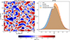 |
Fig. 1. Illustration of the inference of the halo environment distribution p(δ|g). Left: Galaxies traced back to their origin in Lagrangian space (marked as black dots) and with the (smoothed) linear density field, δ, inferred at their Lagrangian locations. Right: Environment distribution (orange histogram) given by the distribution of δ at the galaxy locations which is notably biased relative to the matter distribution, p(δ), (blue histogram and a Gaussian represented as dashed line). The galaxy environment distribution is well approximated through p(δ)f(δ), where here f(δ) is a quadratic polynomial bias function. |
Through Bayes’ theorem, the relation between the galaxy environment distribution and the bias function is given by


This means for example, that the bias function, f(δ), can be investigated in a non-parametric way by measuring p(δ|g) and dividing by the Gaussian background distribution, p(δ), as we will investigate in the companion paper (Stücker et al. 2025).
In this section, we explain how we use probability theory to investigate the properties of the galaxy environment distribution. In particular, we show that the bias parameters are simply related to the moments of this distribution and that probability theory motivates the application of better behaved ‘cumulant bias parameters’.
2.2. Bias estimators
Following up on Equation (6), we can write
We note that in the last line, we made the substitution δ → δ + δ0; also, δ represents the linearly extrapolated overdensity and, hence, it can assume values that are between negative and positive infinity. The latter Equation can be interpreted as an alternative perspective onto the separate-universe experiment: when increasing the background density, the probability of environments is changed by a factor p(δ − δ0)/p(δ), whereas the likelihood of forming a galaxy when presupposing a given environment stays constant.
Now, combining Eqs. (3) and (11), we can evaluate the bias parameters as
where the angled brackets with a ‘g’ subscript indicate an expectation value evaluated over the locations of galaxies (rather than all of Lagrangian space). Furthermore, we can use the fact that p is a Gaussian distribution, for which the derivatives are given by the (probabilisist’s) Hermite polynomials:
so that the bias estimators are:
Here, the subscript ‘so0’ indicates that these estimators are at a ‘spatial order of 0’. In other words, they do not include corrections from higher spatial derivatives such as the Laplacian (as we explain in more detail later in this work). This expression was already used by Paranjape et al. (2013a,b) to measure the bias parameters. It was motivated by its emergence in excursion set frameworks (Musso et al. 2012) and peak statistics (Paranjape & Sheth 2012), but it is clearly also valid outside such frameworks, requiring us to only assume the PBS. On a related note, it is worth mentioning that Szalay (1988) previously proposed expanding the field in terms of Hermite polynomials.
The estimators for the first four bias parameters are expressed as:
2.3. The moment generating function
Equation (14) shows that there exists a simple relation between moments of the galaxy environment distribution and the bias parameters. We can show this in a very general manner. Expanding the Gaussian background distribution, we obtain
Inserting this into Equation (11) yields
where we have labelled t = δ0/σ2. The last term can be identified with the moment generating function,
of the galaxy environment distribution. Therefore, the moment-generating function of the galaxy environment distribution and the separate-universe bias function can be directly converted into each other as follows:
Furthermore, the relation between the moments and the bias parameters, as given by Equation (14) can equivalently be found by taking derivatives of the moment generating function:
It is worth noting that this result may be related to the considerations in White (1979), where in the case of discrete tracers, the moment-generating function of the galaxy count frequency distribution is expressed through the void probability function.
2.4. Cumulant bias parameters
We may further consider how the bias parameters are related to the cumulants of the galaxy environment distribution. In probability theory, the value of cumulants are generally thought to characterise a distribution more independently than its moments. For example, if a distribution has a large first moment ⟨x⟩, then we should also expect that it has large second and third moments ⟨x2⟩ and ⟨x3⟩. However, the first cumulant of a distribution ⟨x⟩ says very little about the second and third cumulants, ⟨(x−⟨x⟩)2⟩ and ⟨(x−⟨x⟩)3⟩, respectively. For example, for a Gaussian distribution the mean is independent of its variance and the third and higher order cumulants are actually zero.
The cumulant generating function is defined as
Cumulants of the galaxy environment distribution are simply given by the derivatives of the cumulant generating function
Therefore, they can be evaluated as:
where we have defined
We notice that the question of whether β2 is above or below zero is a direct indication of whether the variance of the halo environment distribution is larger or smaller than that of the background. We refer to these parameters as ‘cumulant bias parameters’ and they are directly related to the canonical bias parameters bn. Comparing their definition to the canonical bias parameters in Equation (3) shows that they relate to each other exactly in the same way that cumulants relate to moments (compare Equations (22) and (24)). For example, at the first four orders we have:


2.5. Interpretation
Given a set of bias parameters, these relations allow us to directly find the cumulants of the galaxy environment distribution, or alternatively, they allow us to infer canonical bias parameters by measuring cumulants of the galaxy environment distribution.
However, it is also possible to phrase the bias expansion directly in terms of the cumulant bias parameters.
There are several reasons to believe that they may form a better set of parameters than the canonical bias parameters:
-
The cumulant bias parameters are the derivatives of the logarithm of the galaxy density. Therefore, they presuppose the positivity of F and may be better behaved, especially in low density regions.
-
The canonical bias parameters behave similarly to moments of the galaxy environment distribution. For example, we may expect that if b1 is large, automatically b4 will also be large. On the other hand, we may expect β4 to be independent of the value of β1 – just as cumulants are relatively independent of each other.
-
If the galaxy environment distribution has the form of a Gaussian then βn = 0 for all n > 2. On the other hand, all bn would be non-zero in this case. Therefore, if all βn beyond a degreeof 2 are small, this motivates the usage of a Gaussian bias model – where both log F and log f are quadratic polynomials. We show here that this is indeed the case for halos.
Furthermore, we note that the cumulant bias parameters and the probabilistic considerations in this section motivate novel approaches to parameterising the bias function at finite smoothing scales. There are several possible well motivated approaches and we only mention them here in brief, leaving a more thorough investigation to future studies.
The first and most straight-forward proposition is to assume an expansion of the logarithm of the bias function, leading to an exponential of a polynomial


Such a bias expansion would have to be truncated at an even order (if n ≥ 2) and the highest order coefficient must be negative to guarantee a fully normalised probability distribution. By definition, this guarantees the positivity of the bias function which is arguably a desirable property – especially if our intention is to create mocks from a bias model. Furthermore, the resulting distribution would be part of the exponential family which guarantees several desirable properties. The main limitation is that at orders of n > 2, it might be difficult to properly re-normalise the expression analytically4.
This choice is the only general one we know of that guarantees f(δ) > 0 for all values of δ, even if the expansion is truncated. However, there are a few other noteworthy options that do not fulfill this constraint. One option is motivated by the intriguing simplicity of the relation between cumulant generating the function in Equation (23) and F. This motivates to define the bias function directly through the cumulant generating function,
where Km(t) is the cumulant generating function of the matter distribution. This general Ansatz might also be feasible in Eulerian space, but for the Lagrangian case, it is simply  .
.
If the expansion is truncated at an order of n = 2 then this corresponds to a well defined Gaussian bias model, but if it is truncated at a higher order, then it is not easy to find an analytical form of f(δ). However, a numerical expression can be obtained through a Fourier transformation. Unfortunately, such a truncation at higher orders does not lead to a well defined probability density, but instead may have negative function values. In fact the cumulant generating function does not yield a positive probability density function (pdf) for any finite order polynomial of degree n > 2 (Lukacs 1970). However, this does not disfavour this approach over the canonical bias expansion which also yields a negative pdf.
Furthermore, we note that it is an option to phrase the bias expansion relative to a Gaussian distribution that has the correct cumulants up to an order of 2, as follows:
where μg = κ1 = β1σ2 and σg2 = κ2 = β2σ4 + σ2. This is also where the γn start at an order of 3, since the lowest two orders are already specified through the Gaussian. This type of expansion is similar to a truncated Edgeworth series (which is an expansion to approximate distributions with given cumulants).
Finally, we note that it is possible to use the cumulant bias parameters in a classical polynomial bias expansion as well. For example, a third-order expansion that only uses two parameters, assuming β3 = 0 would read

This can be understood as the lower order terms predicting the likely behaviour of higher order terms.
2.6. Multivariate estimators
So far, we have only considered the bias function based on the assumption that the only known aspect of the environment is the density, δ, at the considered location. However, other aspects of the environment may be known, such as the Laplacian,

or higher order derivatives of the density field,

or the tidal field. Since the tidal field is inherently a tensorial quantity, its treatment is slightly more complicated and we therefore discuss this in more detail in Sect. 4.
Assuming that we are dealing only with scalar quantities that describe the environment, we may summarise the environment through a single vector x – for example, if we consider the density and Laplacian as variables we have x = (δ, L)T. The majority of the relations that we have derived in the previous section hold in a similar manner for the multivariate case as well. We do not derive all of them again, since their derivation follows almost completely analogously, however, we do list all the important relations.
Assuming that all the considered environment variables follow from linear operators on the Gaussian random field, their distribution is given by a multivariate Gaussian,
For example, for the case of x = (δ, L)T, which is particularly well motivated by the peak model (Bardeen et al. 1986), we have the covariance matrix:
![$$ \begin{aligned} \mathsf{C }_{\delta ,L}= \left[\begin{matrix} {\sigma _{0}^{2}}&{- \sigma _{1}^{2}} & {\sigma _{1}^{2}} &{\sigma _{2}^{2}}\end{matrix}\right], \end{aligned} $$](/articles/aa/full_html/2025/07/aa51176-24/aa51176-24-eq42.gif)
![$$ \begin{aligned} \mathsf{C }_{\delta ,L}^{-1}= \left[\begin{matrix}\frac{\sigma _{2}^{2}}{\sigma _{0}^{2} \sigma _{2}^{2} - \sigma _{1}^{4}}&\frac{\sigma _{1}^{2}}{\sigma _{0}^{2} \sigma _{2}^{2} - \sigma _{1}^{4}}\\ \frac{\sigma _{1}^{2}}{\sigma _{0}^{2} \sigma _{2}^{2} - \sigma _{1}^{4}}&\frac{\sigma _{0}^{2}}{\sigma _{0}^{2} \sigma _{2}^{2} - \sigma _{1}^{4}}\end{matrix}\right], \end{aligned} $$](/articles/aa/full_html/2025/07/aa51176-24/aa51176-24-eq43.gif)
where σ02 = ⟨δ2⟩, σ22 = ⟨L2⟩ and σ12 = ⟨−δL⟩.
Now, we can conveniently write bias parameters in a matrix form


Here, ⊗ designates an outer product, the power notation in the last line designates a repeated outer product, b1 is a vector, b2 is a symmetric rank two matrix, b3 is a symmetric rank three tensor, and so on. Furthermore, ∇x denotes a gradient with respect to the chosen variables, for example, ∇x = (∂/∂δ, ∂/∂L)T.
It is then straightforward to show
which at the first two orders, can be expressed as:

Importantly, these expressions do not lead to the same bias estimators for the density if a second variable is present that is correlated with the density. For example, if we use the density and Laplacian as variables, we find
for the components of b1 and
for the components of b2, where we have written, for instance, bδδ as a symbol for what was previously referred to as b2. Furthermore, we note that a general form for the Nth density bias parameter is given by
with  . We note that these relations have already been derived through the response of density peaks to large scale perturbations (Bardeen et al. 1986; Mo & White 1996; Desjacques et al. 2010) and were later been shown to apply also to more general tracers (Lazeyras et al. 2016).
The difference between Eqs. (49)–(54) and the estimators from Eqs. (15)–(18) is that they correspond to partial derivatives of the density at fixed values of the Laplacian. The previous estimators are the derivatives of the projected distribution, which is not the same due to the correlation between density and Laplacian. As we see in Sect. 3.3, the new estimators are less scale-dependent, since they are closer to pure partial derivatives with respect to the density (in the separate-universe sense).
We refer to the estimators from Equations (49)–(54) as the estimators with spatial corrections of the second order, whereas the previous estimators are without any spatial corrections (i.e. at the spatial order of 0). It is straightforward to obtain higher order spatial corrections, for instance, by considering the covariance matrix of the distribution of x = (δ, L, P)T with P as in Equation (38). For example, the estimators of density bias parameters at a spatial order of 4 can be expressed as
where σ32 = −⟨δ⋅P⟩ and σ42 = ⟨P2⟩. In practice, it is easier to evaluate such high-order estimators numerically, rather than deriving explicit expressions for them. The covariance matrix may easily be measured from a given linear density field and then used to evaluate the estimators as e.g. in Equation (48), so that in principle it is not very difficult to obtain corrections at any spatial order. Throughout this article, we mainly focus on the estimators of a spatial order of 2, since they are already sufficiently accurate to obtain good measurements of biases, but we have selectively included both lower or higher order estimators throughout this article to demonstrate the convergence.
We note that the estimators with second-order spatial corrections are quite similar in spirit to the considerations by Musso et al. (2012), Paranjape & Sheth (2012), Paranjape et al. (2013b,a) to map scale-dependent measurements of biases as in Equation (14) under the assumption of excursion set (peaks) models to scale-independent large-scale parameters. However, here we can see that such a mapping to the large-scale limit can be done without the assumption of Peak or excursion set models and for spatial corrections of any order. Consider for example that the relation between the zeroth-order spatial estimator and second-order spatial estimator of b1 is given by
Therefore, bL, so2 predicts the scale dependence of b1, so0 and b1, so2 posits a more scale-independent estimate:
We note that this argument can easily be pushed to higher spatial orders:
The additional cost of our approach (e.g. in comparison to Paranjape et al. 2013a) is that, beneath the density, also the Laplacian has to be evaluated in Lagrangian space, but the benefits are model-independence and a much reduced mathematical complexity.
2.7. Multivariate cumulants
Analogously to the monovariate case, we define multivariate cumulant bias parameters as
which immediately leads to


where we gave β3 in index notation, since the central term is difficult to express in vectorial notation. We note that this leads to the same relations between the density cumulant biases and their canonical biases as in Equations (27)–(30), but it also includes additional relations, such as:

Finally, the relation between the separate-universe bias function and the moment and cumulant generating functions is analagous to the expression in Equations (21) and (23), given by
which can be differentiated to show that the cumulants are given in an easy form through the cumulant bias parameters, for instance,

However, instead of measuring directly the cumulants of the galaxy environment distribution and inverting Equations (65)–(67), it is in practice simpler to instead define the variable,

We then measure its cumulants, κu, which relate to the cumulant biases as
where a and b indicate the indices of the non-zero variables in the second-order case.
We show in Appendix A that it is also possible to derive similar estimators if the density field was filtered with a function different than a sharp k-space filter. The only additional complication in that case that it is necessary to account for the correlation matrix between the smoothed large scales and unsmoothed small scales. However, for simplicity, we focus only on measurements with the sharp k-space filter in this work.
3. Density bias measurements
In this section, we explain our evaluation of the Lagrangian density bias parameters for different sets of halos. We want to verify the consistency of our estimators by comparing them to the vast literature available on the subject. Furthermore, we also compare the canonical bias parameters, bn, with the cumulant bias parameters, βn.
3.1. Simulation
For the analysis through this paper, we used a single cosmological box simulation with high resolution. This simulation is part of the ‘BACCO simulation project’ that was first introduced in Angulo et al. (2021). It has a box size of L = 1440h−1Mpc with 43203 particles leading to a mass resolution of mp = 3.2 × 10⁹ h−1 M⊙. The cosmological parameters are Ωm = 0.307, ΩΛ = 0.693, Ωb = 0.048., ns = 0.9611, σ8 = 0.9, h = 0.677 which are similar to the Planck Collaboration VI (2020) cosmology except for the roughly 10% larger value of σ8. By default we use this simulation at a scale-factor of a = 1.08, corresponding approximately to a = 1.
To identify halos, the simulation code uses a modified version of SUBFIND (Springel et al. 2001), which first identifies halos via a friends of friends (FoF) algorithm and subsequently calculates for each FoF group, the mass, M200b, in a region that encloses 200 times the mean density of the Universe.
3.2. Bias measurements
We defined sets of biased tracers by considering halos selected by their mass. For this, we considered 21 equally log-spaced halo masses between 1012 h−1 M⊙ and 1016 h−1 M⊙ and for each halo mass, we considered all halos with masses in the range of
![$$ \begin{aligned} M_{200b} \in [M_i / 1.25, M_i \cdot 1.25 ]. \,\, \end{aligned} $$](/articles/aa/full_html/2025/07/aa51176-24/aa51176-24-eq74.gif)
To evaluate our Lagrangian bias estimators, we only need to know the linear field evaluated at the Lagrangian locations of the tracers. We approximated the Lagrangian location of each halo through the Lagrangian coordinate of its most bound particle. Since the simulation started from a Lagrangian grid, the Lagrangian origin of the most bound particle can easily be inferred from its id imb as
where Ngrid = 4320 is the number of particles per dimension.
We know the linear density field of the simulation through the initial condition generator. To save on the computation time, we can create a low resolution grid representation of the linear density field with Nlin3 grid points. For fields different than the linear density field, we additionally multiply by the correct operator (e.g. −k2 for the Laplacian) in Fourier space. We created a smoothed version of this field by multiplying with a sharp k−filter in Fourier space
where Θ is the heavy-side function and we tested, for each measurement, different damping scales kd ∈ [0.1, 0.15, 0.2, 0.25, 0.3] h−1 Mpc. We then deconvolved this field with a linear interpolation kernel and interpolated it to the Lagrangian locations of our tracer set. We chose an Nlin value that is sufficiently large that the resulting interpolated values are virtually independent of this discretisation; for instance, Nlin = 183 at kd = 0.1 h−1 Mpc and Nlin = 549 at kd = 0.3 h−1 Mpc.
With the linear densities at the Lagrangian locations of tracers, it is easy to evaluate the zeroth-order spatial estimators of the biases by averaging as in Equation (14). However, for higher spatial order estimators we also need to know the values of the Laplacian (Eqs. (49)–(53)) or that of the fourth derivative (Equation (55)). The Laplacian is inferred by multiplying the linear density field in Fourier space by −k2 and then interpolated to the tracer locations. Other variables such as the fourth derivatives can be evaluated in a similar manner. This allows us to evaluate any of the bias estimators (from Sect. 2) directly as simple expectation values over tracers. We note that this is a major difference compared to the measurement process in Paranjape et al. (2013a), where the zeroth-order spatial estimators, as those in Equation (14), were evaluated, but then mapped to scale-independent parameters through peak theory arguments.
To estimate the covariance of a set of measured bias parameters we use a Jackknife technique. For this we divide the box in Lagrangian space into Njk3 subboxes with Njk = 4. We perform 64 measurements of the vector of bias parameters bi by subsequently leaving out all tracers in one of the subboxes. Then we estimate the covariance through
It is worth noting that the Jackknife estimator results in a more reliable estimate of the uncertainty of the measurement than, for instance, a simple bootstrap would yield. When comparing these estimators we found that the Jackknife gives larger (more conservative) error estimates, since it also accounts for the uncertainty induced by cosmic variance, which is sampled by leaving out spatially correlated parts of the data sets.
3.3. b1 and the scale dependence of estimators
In Figure 2, we show the measurements of b1 for halos as a function of M200b using the estimator from Equation (15) without spatial corrections (top panel) versus the estimator from Equation (49) with spatial corrections at the second order (bottom panel). The dashed lines indicate the fitting function from Tinker et al. (2010) evaluated for the cosmology of our simulation.
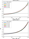 |
Fig. 2. b1 as a function of halo mass using the estimators from Equation (15) at the top and Equation (49) at the bottom, measured at different damping scales (different coloured regions). The shaded regions indicate the 1σ certainty region of the estimators. Using the b1 estimator that includes the Laplacian correction increases the uncertainty of the b1 estimates, but reduces the dependence on the damping scale, leading to a good agreement across different scales. |
As expected, halos of large masses M ∼ 1015 h−1 M⊙ are highly biased b1 ∼ 3, whereas low-mass halos (M ∼ 1012 h−1 M⊙) have an even slightly negative (Lagrangian) bias. The zeroth-order spatial estimators have a very small degree of statistical uncertainty, but exhibit a significant scale dependence and are inconsistent across different damping scales. On the other hand, the estimators with a spatial order of 2 have a larger statistical uncertainty, but seem consistent across different damping scales – except at very large kd and large halo masses; in this case, some scale dependence becomes visible, probably indicating the effect of higher spatial-order terms.
Our second-order spatial measurements agree at all scales well with the fitting function from Tinker et al. (2010). While they lie systematically about 5% below this fit, this is within the quoted uncertainty of the Tinker et al. (2010) fit and a similar difference can be seen in Lazeyras et al. (2016). In comparison to other studies at z = 0 (e.g. Lazeyras et al. 2016), we have lower bias values at the same masses (e.g. b1 ∼ 0.5 at 1014 h−1 M⊙ instead of b1 ∼ 1) because of the later time (z = −0.08) and relatively high variance (σ8 = 0.9) of our simulation.
To further highlight the difference in the scale dependence of the estimators, we show in Figure 3 the error Δb1 in b1 measurements as a function of damping scale for a few different halo masses. Here, we phrase the error Δb1 = b1 − b1, ref relative to the second-order spatial estimator at kd = 0.2 h Mpc−1 as b1, ref. As expected, the zeroth-order estimator seems to approach the selected reference value on large scales. However, the zeroth-order second-order spatial estimator exhibits a significant scale dependence, whereas the second-order spatial estimators are almost scale-independent, except for the largest one at kd ≳ 0.25 h Mpc−1. We also show measurements with the fourth-order spatial estimator from Equation (55), which are scale-independent to even smaller scales, showing that the measurements converge well with adding higher order spatial corrections. However, for getting a good estimate of the bias parameters it seems sufficient to use the second-order spatial estimator at scales of kd ≲ 0.2 h Mpc−1, which bears a similar accuracy in measurement, for instance, akin to evaluating the fourth-order spatial estimator at kd ∼ 0.3 h Mpc−1.
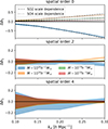 |
Fig. 3. Scale dependence of the error in b1 estimates for different halo mass selections. The error is expressed relatively to the measurement with spatial order of 2 at |
We can estimate the scale dependence of the zeroth-order spatial estimator, as shown in Equations (56) and (57). We mark the estimated scale dependence of the zeroth-order spatial estimators using the second-order spatial bias parameters measured at kd = 0.2 h Mpc−1 as dashed lines in Figure 3 and using the fourth-order spatial parameters from kd = 0.3 h Mpc−1 as dotted lines. The scale dependence of the zeroth-order spatial estimator is predicted quite well, showing that the consideration of the Laplacian introduces a correction of the order of σ12/σ02, which scales approximately as kd2 and including of the fourth derivatives provides additional corrections that become relevant on even smaller scales.
Our measurements therefore confirm the results from previous studies that including the Laplacian is vital to recover scale-independent bias on large scales (Paranjape et al. 2013a; Lazeyras et al. 2016). Furthermore, if the modelling is pushed to small scales kd ≳ 0.25h the inclusion of additional higher spatial derivative terms may prove beneficial.
3.4. b2 versus β2
The first cumulant bias parameter that is different from the canonical bias parameter of the same order is β2 = b2 − b12 where b1 = β1. Since there is a one-to-one relation between (b1, b2) and (β1, β2) it might seem that there should not be any advantage by using β2 over b2 as a parameter when fitting datasets. However, here we show that β2 seems to be more independent of β1 than b2 of b1, especially when their covariance matrix is considered.
In Figure 4, we show the measured co-evolution relation between b2 and b1 (left) versus the co-evolution between β2 and β1 (right) for the second-order spatial estimators. In comparison, we also show the co-evolution relations measured by Lazeyras et al. (2016) as a dashed line, which seems to match our measured relation well up to kd ≲ 0.15 − 0.2 h Mpc−1, showing that our method for measuring the bias parameters is indeed able to recover the correct large-scale limit of the bias parameters.
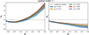 |
Fig. 4. b2 and β2 as a function of b1 = β1 using the second-order spatial estimators. The black dashed line is the b2(b1) relation inferred by Lazeyras et al. (2016) from separate-universe simulations. The second-order spatial estimators seem consistent with the literature co-evolution relation down to damping scales of kd ∼ 0.15 − 0.2 h Mpc−1. It is noteworthy that β2 < 0 appears to always hold, which means that the width of the galaxy environment distribution p(δ|g) is always smaller than that of the background p(δ). Therefore, the cumulant bias parameter β2 − β1 relation appears slightly simpler than the b2 − b1 relation. |
We note that for halos we find β2 < 0 across all masses and with high statistical significance. This means that the width of the halo environment distribution p(δ|g) is smaller than the width of the background distribution p(δ) – showing that halo formation is more selective than a random distribution. Possibly, the assumption β2 < 0 could be used to limit the considered prior range when fitting certain galaxy surveys. However, it is difficult to anticipate whether this should hold for every possible set of galaxies.
Furthermore, we note that the co-evolution relation between β2 and β1 is monotonic and roughly linear. For b1 ≳ 2, it satisfies |β2|< |b2|. Therefore, β2 versus β1 seems slightly simpler than the b2 to b1 relation.
The benefit of using β2 as a parameter is even more evident when considering the covariance matrix of the measurements. In Figure 5 we show the uncertainty of the b2 measurements (solid lines), versus the uncertainty of the β2 measurements. Comparing different damping scales shows that the inclusion of smaller scales in the measurements decreases the statistical uncertainty (but increases systematic error). In all cases and especially at high values of b1 the uncertainty of β2 is significantly smaller than that of b2. This is so, since b2 and b1 are more correlated than β2 and β1.
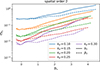 |
Fig. 5. Uncertainty of b2 measurements (solid lines) and β2 measurements (dashed lines) as a function of b1 for different damping scales. The uncertainty of β2 is significantly smaller than of b2 for high values of b1. |
To highlight this we show in Figure 6 the correlation coefficient
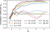 |
Fig. 6. Correlation coefficient α12 between the b1 and b2 measurement (solid) and the β1 and β2 measurement (dashed). Note: β2 as a parameter is much more independent of the value of b1 than b2. |
where C is the covariance matrix between b1 and b2 or β1 and β2. For b1 ≫ 0 the correlation coefficient of (b1, b2) is quite large, even close to 1 in some cases. On the other hand, the correlation coefficient of (β1, β2) is quite small and seems on average consistent with 0. Therefore, measurements of b1 are quite entangled with b2, but not so much with β2. While we do not show it here, we have found that this is also the case for higher order correlations, for instance, those of (b1, b3) versus (β1, β3).
This can be understood when considering the difference between moments and cumulants of a probability distribution. For instance, if we knew with respect to a certain distribution p(x) that it has a large first moment ⟨x⟩, then we might also expect that the second moment ⟨x2⟩ is large. On the other hand, knowledge about the mean of a distribution, is very uninformative about its width – that is its second cumulant σx2 = ⟨(x−⟨x⟩)2⟩ = ⟨x2⟩ − ⟨x⟩2. In the same sense, we would expect the cumulant bias parameters to be more independent of each other than canonical bias parameters.
3.5. Higher order biases
While the second-order cumulant bias β2 has already slight advantages over b2 as highlighted in the last section, the benefits are even more significant at higher orders. Here, we compare the behaviour of b3 and b4 with the behaviour of β3 and β4.
In Figure 7, we show b3, b4, β3, and β4 as a function of b1 for the second-order spatial estimator. The uncertainty of the measurements of b3 and b4 are much larger than for b2 so that we hardly find any signal at kd ∼ 0.1 h Mpc−1. However, at kd ∼ 0.15 h Mpc−1 we can find a meaningful signal and it is consistent with the b3 measurements of Lazeyras et al. (2016).
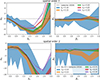 |
Fig. 7. Co-evolution relations of higher order bias parameters b3 and β3 (top) and b4 and β4 (bottom) for the second-order spatial bias estimators. For b4 we indicate as a dashed line a prediction that follows from combining the Lazeyras et al. (2016) measurements of b1, b2 and b3 with Equation (30) when using β4 = 0. Strikingly, β3 and β4 are extremely close to 0 – independently of the value of b1. |
Strikingly, the value of β3 is extremely small in comparison to b3 and seems approximately consistent with 0. It is noteworthy that this is not only the case for scales where b3 is reasonably scale independent (kd ≲ 0.15 h Mpc−1), but it is also so for much smaller scales. There does not seem to be any noteworthy relation between β3 and β1. Furthermore, the co-evolution relation measured by Lazeyras et al. (2016) seems consistent with β3 = 0. Therefore, we could summarise the third-order co-evolution relation through the relation we get by using β3 = 0 in Equation (29):
Similarly, we find for β4 an apparent independence of β1 and consistency with zero across different scales. Assuming β4 = 0 in Equation (30) leads to the co-evolution relation between b4, b3, b2, and b1 given by

We mark this relation with the measurements of b1, b2, and b3 from Lazeyras et al. (2016) as a dashed line in the bottom left panel of Figure 7. This seems in good agreement with the measured b4.
We conclude that at an order of n ≥ 3, the cumulant bias parameters are very close to 0. The co-evolution relations at these orders can be summarised simply through βn = 0. We might therefore suggest that high-order co-evolution relations do not represent any physical insights, but rather highlight that the canonical bias parameters form a suboptimal, deeply entangled basis.
Further, the fact that all the cumulant biases beyond an order of 2 are close to zero indicates that the galaxy environment distribution is very well approximated by a Gaussian distribution. We plan to investigate the possibility of a Gaussian bias model in Stücker et al. (2025), where we also explain how this fact may arise naturally from the Gaussianity of the background distribution.
3.6. Laplacian bias
In Figure 8, we show the Lagrangian Laplacian bias parameter as a function of halo mass, as inferred from the estimator in Equation (50). The Laplacian measurements have a much stronger scale dependence than our previous measurements of density bias parameters. However, it seems that at masses M ≲ 3 × 10¹³ h−1 M⊙ the scale dependence disappears and a reliable measurement is obtained.
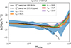 |
Fig. 8. Lagrangian Laplacian bias bL as a function of halo mass. At masses M ≲ 3 × 10¹³ h−1 M⊙ the scale dependence of the bL measurements disappears and they agree well with the fits of the Eulerian Laplacian bias from Lazeyras & Schmidt (2019). |
We compare our Lagrangian measurements with the Eulerian measurements of Lazeyras & Schmidt (2019). In general, the relation between the Lagrangian and Eulerian Laplacian bias depends on velocity bias (e.g. Desjacques et al. 2018). The velocity bias bs quantifies the difference between the displacement field of matter s and galaxies sg and gets as first-order contributions of the form
Therefore, the galaxy density can get an extra contribution proportional to the divergence of this field, that scales as L = ∇2δ. However, for our set of tracers sg = s by definition, so that bs = 0 and we simply assume that their Lagrangian and Eulerian Laplacian biases are identical or at least very similar.
In the reliable range of M ≲ 3 × 10¹³ h−1 M⊙, it seems that our measurements agree well with the linear and the quadratic (in halo radius) fit that was inferred by Lazeyras & Schmidt (2019) for the Eulerian Laplacian bias. Therefore, we confirm that the Laplacian bias is negative for halos and that it can plausibly have amplitudes of the order of bL ∼ −20 Mpc2 h−2. However, we leave more detailed considerations to future studies. In principle, more accurate measurements could be obtained by consideration of higher order corrections and through measurements at higher redshifts.
3.7. The scale-split break-down scale
The core assumption of the bias formalism is the separation of scales: the formation of galaxies and halos is assumed to depend only on the properties of the Lagrangian environment on some small length scale. Larger scale perturbations are only relevant as far as they determine the distribution of small scale environments. We refer to this as the ‘scale-split’ assumption.
This assumption makes it possible to define scale-independent bias parameters. For example, b1 describes how the likelihood of forming a galaxy responds when changing only the linear density contrast δ of the relevant smaller scale environment, while keeping other aspects (e.g. L) constant. As all larger scale density perturbations affect this aspect in the same way b1 is independent of scale.
Physically, the scale-split assumption has to become invalid for sufficiently small smoothing scales. For example, halo formation may respond differently to perturbations that are smaller than their Lagrangian radius, than to those which are larger.
Here, we want to show that the scale-split assumption also becomes mathematically inconsistent beyond some scale for a given set of variables: Recall that we have shown in Equation (25), how κ2, the variance of the galaxy environment distribution, changes with scale. The predicted variance is only well defined, if
This becomes zero if σ = σmax, δ. Mathematically, at this scale, the environment distribution and the bias function have to become Dirac-delta functions. We may understand σmax as the scale where (formally) all information that is relevant for galaxy formation has been accounted for and the biasing becomes deterministic in density.
Beyond this scale, the PBS predicts a galaxy environment distribution with negative variance – making any density-only bias model mathematically inconsistent. It may seem as if it was possible to set up expansion bias models for arbitrary high σ, but this is only so, since the negativity of the bias function makes it formally possible to have a negative variance. Actual galaxies will strictly obey κ2 > 0 and therefore, the response of density-only models has to become scale-dependent latest at σmax, δ – but likely already earlier. We call this the ‘scale-split break-down scale’.
The break-down scale is different if additional variables are considered. For the multivariate distribution of density and Laplacian (δ, L), we have to require the covariance matrix of the galaxy environment distribution to be positive and semi-definite. For this, it is at least necessary to have:
which appears slightly more complicated, but it will also be violated at some finite damping scale.
To measure the break-down scale, we infer for each halo mass the bias parameters at three different scales kd ∈ (0.15, 0.2, 0.25) h Mpc−1. Then, we evaluate the co-variance matrix of the background distribution at 500 different equally log-spaced damping scales between 10−3 h Mpc−1 and 101 h Mpc−1 and determine the earliest damping scale kmax where the covariance is large enough to violate Equation (80) or Equation (81). We show the corresponding results as shaded contours in Figure 9, where we additionally mark the characteristic wave-number of halos as:
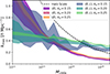 |
Fig. 9. Maximum damping scale where the PBS can be valid and bias scale-independent. The three reddish contours show the break-down scale of density-only bias models, estimated with bias parameters measured at different scales, and the three green-blueish contours show it for (δ, L) bias models. The black dashed line shows the wavenumber associated with the Lagrangian radius of halos. The break-down scale is consistent across different measurements and only seems to scale strongly with halo radius for the (δ) case. |

where Rhalo is the Lagrangian radius that encloses the halo mass, M200b.
Comparing the measurements at different damping scales, we find that the inferred scale is reasonably converged with the scale that we measured the bias parameters at. The density-only break-down scale is typically a factor two smaller than khalo and seems roughly proportional to it. We therefore conclude that any Lagrangian local in matter density (LLIMD) bias model with scale-independent bias parameters has to break down at a length scale roughly a factor two larger than Lagrangian radii of the considered halos5.
On the other hand, the (δ, L) case shows a notably different break-down scale. It scales only weakly with halo mass and it ranges only between kmax ∼ 0.3 − 0.5 h Mpc−1. Note that this corresponds roughly to the Lagrangian scale of halos with M ∼ 2 × 10¹⁴ h−1 M⊙, where b1 ∼ 1. For halos above M ≳ 3 × 10¹³ h−1 M⊙ including the Laplacian increases kmax relative to the density-only case, but for lower masses, it decreases it.
Comparing with the right panel of Figure 4, we notice that the bias parameters already become scale-dependent at notably smaller damping scales than kmax. For example, for M200b ∼ 1015 h−1 M⊙ with b1 ∼ 3, the measurements of β2 are already scale-dependent beyond kd ≳ 0.15 h Mpc−1, whereas the mathematical break-down scale is kmax ∼ 0.3 h Mpc−1. We therefore suggest that considerable care should be taken when setting up bias models close to the break-down scale. This is particularly relevant for hybrid methods, which might, in principle, allow for galaxy clustering to b described at notably smaller scales than are usually considered in a perturbative schemes (e.g. Modi et al. 2020; Zennaro et al. 2022).
4. Estimators for tensorial bias parameters
In Sect. 2, we explain how we inferred the general estimators of bias parameters associated with scalar variables (e.g. the density and Laplacian) with spatial corrections of any order. In Sect. 3, we show how these can be used to obtain reliable bias measurements from a single simulation.
However, the theory in Sect. 2 does not explain how to obtain estimators for parameters such as the tidal bias, bK2, which is defined as the response to
where ϕ is the displacement potential, I2 is the unit matrix, and K is the traceless tidal tensor. In this section, we present a general scheme to measure the related bias parameter bK2 and any other bias parameters that follow from contractions of derivatives of the potential field.
To achieve this, it is not optimal to consider directly the distribution of such scalar contracted quantities, since these distributions may get quite complicated. For example, p(K2) is not a Gaussian distribution, but rather a χ2 distribution with five degrees of freedom. Furthermore, it is not immediately obvious how to define partial derivatives with respect to such variables, since partial derivatives may depend on what other terms are kept fixed. For example, it is not clear how a term like K3 = tr(K⋅K⋅K) would be derived with respect to K2. It seems therefore difficult to generalise Equation (12) in this manner.
However, a clear and general framework for measuring such ‘tensorial’ bias terms can be developed by instead considering the full (quite high dimensional) distribution of the tidal tensor and its derivatives. Since the potential field of the early Universe is a Gaussian random field, these must follow a multivariate Gaussian distribution so that it is easy to compute derivatives of the distribution function in a general manner. The resulting ‘bias tensors’ can be decomposed into isotropic tensors that each have a one to one correspondence with traditionally used bias parameters. In this section, we introduce the needed mathematical notions step by step and will provide estimators for a few selected bias terms.
4.1. Tensorial bias expansion
We write the bias expansion in tensorial form as

Here, again, F = ng/ng, 0 (in a separate-universe sense) and

where BT is a canonical bias tensor of rank of 2, BTT of rank of 4, BS of the rank of 3, and so on. This is also where an omitted product sign indicates a product over the indices of the last fully symmetric part of the first tensor and the first fully symmetric part of the second tensor. For example:
where we can use  to explicitly denote the number of dimensions that are contracted.
We note that just as before, the bias tensors correspond to derivatives of the large-scale bias function, for instance,
4.2. Isotropic tensors
Due to the isotropy of the Universe, each of the bias tensors has to be isotropic. That means that a bias tensor should be identical when measured from a rotated frame of reference. For example, it has to be

for any rotation matrix U. From this, it follows immediately that BT has to be proportional to the unit matrix I2 (where the proportionality constant is equal to b1). In general, a rank n tensor A is isotropic if it holds for any rotation matrix, U:

Here, we have used Einstein’s sum convention, where the rotation matrix is applied to each index of A individually. To express whether some tensor is isotropic, we define 𝕌n as the space of all tensors that are isotropic and of a rank, n.
In general, all isotropic tensors can be decomposed in index notation through different combinations of the Kronecker-delta symbol δij and the Levi-Civita symbol, ϵijk. For example

where a, b, c ∈ ℝ. A compact way of writing the same type of statement can be:

which signifies that 𝕌4 is the space of tensors that can be reached through linear combinations of the indicated tensors and we say that these are basis tensors of 𝕌4.
It is easy to see that we should be able to decompose each of the bias tensors into a small number of independent scalars that multiply the basis tensors and that correspond to traditional bias parameters. However, before performing such a decomposition we need to further consider the symmetries of the tensors.
4.3. Symmetric isotropic tensors
Since the bias tensors correspond to derivatives of a scalar function with respect to symmetric tensors, they have to obey the same symmetries. For example, the tensor BTT has to be symmetric in the first two and last two indices6:

Therefore, BTT cannot be every tensor from the tensorspace 𝕌4, but only from the subspace 𝕍22 ⊆ 𝕌4 of isotropic rank four tensors that have the 2, 2 symmetry.
To formalise this, we define 𝕍n ⊂ 𝕌n as the space of all isotropic tensor of rank n that are additionally fully symmetric under any permutation of indices, specifically:


We note that 𝕍3 = {0}, namely, the only symmetric rank three isotropic tensor is 0. Furthermore, we define 𝕍nm as the space of all isotropic tensors of rank n + m that are symmetric in the first n indices and the last m indices. For example,

To find a basis for some symmetric isotropic tensor space of rank n, we can consider all basis tensors of 𝕌n, symmetrise these and then discard any tensors that are duplicate or zero. We define the symmetrisation operator Sn which symmetrises a tensor in n indices. For instance, we have:

Furthermore, we defined a double symmetrisation operator, Snm, that symmetrises the first n indices and the last m indices. For example, the effect of S22 onto a rank four tensor M is given in the index notation by
It acts on the basis tensors of 𝕌4 in the following ways:

where we have assumed that δij is itself symmetric. The symmetrised second and third basis tensor are identical. Therefore, 𝕍22 has (unlike 𝕌4) only two basis tensors:
The main difference between δijδkl and the two tensors δikδjl and δilδjk is that the delta symbols used to define δijδkl each connect internally inside the groups of symmetric indices and have no connections between the groups. (Recall that i ↔ j and k ↔ l are to be symmetrised.) However, δikδjl and δilδjk each have zero group internal connections, but two connections between the symmetry groups. In fact, the symmetrisation operation identifies all terms that have the same number of intra- and inter- group connections and therefore we only need to consider how many independent possibilities exist to connect the symmetry groups to identify the basis tensors of any space, 𝕍mn. We can therefore represent the basis tensors of each tensor space through a simple diagram as illustrated in Figure 10. We label these tensors through a symbol that shows the number of inter group connections in the index:
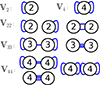 |
Fig. 10. Graphic representation of the isotropic tensors that form a basis for a few selected isotropic tensor spaces with symmetries. All basis tensors of a space with given symmetry can be constructed by considering the number of different ways that the symmetry groups can be connected. In this figure each circle with number n represents a group of n fully symmetric indices and each connection represents one delta symbol (that can either connect two indices from the same group or from two different groups). |


We explain in Appendix B.1 how to construct tensors with three or more symmetry groups. For these cases the procedure is mostly analogous, but it additionally needs to be considered whether there is symmetry with respect to permutations of the different symmetry groups.
4.4. Orthogonal basis
The basis tensors highlighted in the last section are sufficient to uniquely decompose the bias tensors. However, it is advantageous to define the basis tensors in such a way that they are orthogonal to each other.
For example, we can decompose an isotropic tensor M ∈ 𝕍22 as
Its full contraction with I22 is


which includes contributions of both A and B. We could infer A and B from M by additionally contracting with I2 = 2 and then solving the resulting system of equations.
However, it would be desirable to have a simple way of finding the coefficients. Therefore, we define an orthogonal basis such that
where the contraction goes over the full rank r of Ja and Jb (which must have equal rank). Such a basis can be found through Gram-Schmidt orthogonalisation and is for example given for 𝕍22 by:

Then we can easily find the coefficients as
We note that the coefficients inferred in this way are different than the A and B and the chosen basis will also affect the inferred bias parameters.
It is worth noting that a decomposition of a bias tensor into different bases,
corresponds to different independent scalar variables appearing in the bias expansion. For example, if we track the corresponding term from Equation (85), we find
Thus, the non-orthogonal basis leads to δ and T2 as independent terms, whereas the orthogonal basis leads to using δ and K2 as independent terms. The corresponding bias parameters can be directly identified as bJ22 = b2 and  .
.
We list an overview of the orthogonal basis tensors that we use here in Table 1. While it is possible to derive the full algebra of products between isotropic tensors from the index representations, this is rather cumbersome. Therefore, we have written a short code that creates explicit numerical representations of these tensors and with which it is easy to evaluate (and decompose) different types of products of these tensors. We use this together with the symbolic computer algebra system SYMPY (Meurer et al. 2017) to systematically compute symbolic representations of expressions in the following sections. This code is openly available7.
Orthogonal basis tensors that we consider here.
4.5. Bias estimators
Given the orthogonal basis tensors, we define the tensorial bias parameters through
where the rank of JX is 2N. While for scalar terms, as in Equation (3), the bias parameters are simply given by derivatives of the galaxy number with respect to the corresponding scalar, more generally we define bias parameters for any tensorial terms as derivatives of the galaxy number with respect to the tidal tensor (or higher spatial order tensors) that are contracted with the corresponding isotropic tensor.
In complete analogy to Equation (46) it follows that these parameters can be estimated as
where p is the full distribution of the tidal tensor, T.
Bias terms corresponding to higher spatial derivatives like R and S can be defined analogously.
4.6. Tidal bias
We show in Appendices B.2 and B.3 that the distribution of the tidal tensor is given by
where CT+ (the generalised inverse of the covariance matrix, as explained in the Appendix) is given by
Taking derivatives yields
and we find
where we used the inner product between two isotropic tensors:  . We evaluated the terms of this type systematically with numerical representations as described in Sect. 4.4. Naturally, this estimator of bJ2 = b1 is consistent with the one that we have inferred previously in Equation (15).
At the second order, we find the following estimators:

We note that conventionally the bias parameter, bK2, is defined so that it appears with a pre-factor K2 in the bias expansion, whereas our parameter bJ2 = 2 appears with a factor  in the expansion (after contracting the corresponding tensors), so that it is
  . Although we think that our fore-factor convention makes more sense in principle, since bJ2 = 2 corresponds to a second derivative term, we still present our results in terms of the conventional notation (e.g. bK2) throughout this paper.
We note that just as the large-scale value of δ/σ2 at an object’s location is motivated by Equation (15) and sometimes called the ‘bias-per-object’ (e.g. Paranjape et al. 2018; Contreras et al. 2023), we could refer in a similar manner to the value of
as the value of the ‘tidal bias-per-object’.
Just as estimators with spatial corrections could be obtained for the density biases by considering the joint distribution of p(δ, L), we can obtain higher spatial order estimators for the tidal bias by considering the joint distribution of second and fourth potential derivatives p(T, R) and evaluating Equation (125) for this distribution. We show how we derived the bias estimator for this case in appendices B.5 and B.6. The resulting estimator is:

where
and  .
.
4.7. Estimators for third derivative terms
The distribution of third derivatives of the potential S is derived in Appendix B.4 and is given by a multivariate Gaussian with the generalised inverse covariance matrix
We note that it is fine to consider the third spatial derivatives independently of the second derivatives, since the joint distribution factorises as:
We find bias estimators by evaluating Equation (125) as:
where
and where we note again that conventions may differ by a factor 2 so that we have, for instance, bJ3 − 3 = 2b(∇δ)2 if b(∇δ)2 is the bias parameter that would be multiplied (∇δ2) without any fore-factor in a bias expansion.
4.8. Tensorial cumulant biases
As for the scalar case, it is possible to define tensorial cumulant bias parameters instead of tensorial canonical bias parameters. Unfortunately, interesting differences arise only at orders that are higher than the ones that we have considered here. However, for the benefit of future studies, we still want to briefly line out, how to define tensorial cumulant biases.
Analogously to Equation (85), we considered a tensorial expansion of log F as

Taking derivatives at zero and identifying coefficients yields the relations


To decompose this into isotropic tensors we may contract these equations with the isotropic tensors to find the relations


This is consistent with what we derived earlier. Tensorial cumulant biases become more interesting at third order, where third derivative of the bias Function yields

If we contract this with the isotropic tensor S222(J2 = 2 ⊗ J2), we have

Therefore, if the full multivariate bias function is close to Gaussian, also tensorial bias parameters of this form should be expected to be close to zero. Dealing with such objects goes beyond the framework of this study and we set this aside as an interesting proposition for a future work.
5. Measurements of tensorial bias parameters
In this section, we use the estimators derived in Sect. 4 to perform measurements of tensorial bias parameters. Here, we focus on the tidal bias, bK2, and on the biases associated with the third potential derivatives,  and bJ3 ≡ 3. For the tidal bias, we have additionally derived the estimator with spatial corrections of the order of 2, so that we can use it to validate that the presented theory indeed behaves as expected. Furthermore, we chose to briefly check the effect of assembly bias on bK2, which has previously been reported to be quite significant. For these measurements, we used the same simulations and jackknife technique (described in Sects. 3.1 and 3.2).
5.1. Tidal bias
We measured the tidal bias,  , with the estimators from Equation (133) at a zeroth-spatial order and Equation (135) at a spatial order of 2. We show the results as a function of mass in Figure 11. The zeroth-order estimator exhibits a strong scale dependence at scales kd ≳ 0.15 h Mpc−1. However, overall it seems that the tidal bias is very small in amplitude and that a slightly negative Lagrangian tidal bias is preferred at high halo masses. On the other hand, the second-order spatial estimator has a much lower scale dependence and seems mostly consistent across different damping scales, potentially with a slight inconsistency at very high halo masses and large kd. This comes at the price of a significantly increased uncertainty in the measured bias values. However, this demonstrates that the estimators we derived in Sect. 4 do indeed behave the way we would expect. More precise measurements of the tidal bias could easily be obtained by employing a larger simulation volume or by averaging over several realisations.
In Figure 12, we show the co-evolution relation between bK2 and b1. Here, we show for each estimator only the smallest two scales that appear reasonably unbiased in Figure 11. These are kd = 0.1 h Mpc−1 and kd = 0.15 h Mpc−1 for the zeroth-order spatial estimator and kd = 0.25 h Mpc−1 and kd = 0.3 h Mpc−1 for the second-order spatial estimator. It is noteworthy that the estimators of different orders are in agreement with each other. For the larger kd values, the estimators have smaller error bars, but do appear slightly biased at large values of b1 ≳ 2. A rough approximation to the observed functional shape is given by
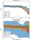 |
Fig. 11. Tidal bias as a function of mass and for different damping scales measured with the zeroth-order spatial estimator (top) versus the second-order spatial estimator (bottom). The second-order spatial estimator exhibits significantly reduced scale dependence at the price of increased error bars. |
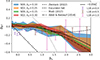 |
Fig. 12. Co-evolution relation bK2 versus b1. Coloured shaded regions are our measurements and error bars show the measurements from Lazeyras & Schmidt (2018). Black lines include measurements from Zennaro et al. (2022), Modi et al. (2017) and Abidi & Baldauf (2018), an excursion set prediction from Sheth et al. (2013) and an approximation that we propose as bK2 = −0.05b12. |
However, the uncertainty is certainly quite high. However, in comparison to some previous literature estimates, we find very small values of bK2. The first measurement that we compare with is from Modi et al. (2017). Their relation is stated for Eulerian bias parameters bK2E(b1E) and we convert it to a Lagrangian relation via b1 = b1E − 1 and bK2 = bK2E + 2/7b1 (Sheth et al. 2013; Desjacques et al. 2018). Similar to other studies (Lazeyras & Schmidt 2018; Zennaro et al. 2022), we find a strong disagreement between our measurements and the Modi et al. (2017) measurements. Furthermore, we show as a dashed line in Figure 12 the co-evolution relation of the tidal bias that was presented in Zennaro et al. (2022). This relation has been measured at very small scales k ∼ 0.7 h Mpc−1 and is not really expected to accurately represent the large-scale tidal bias. However, it is interesting to see that the large-scale tidal response that we measure here is so much weaker than the response that can be measured at small scales. Next, we made a comparison with the excursion set prediction from Sheth et al. (2013) parameterised as  . This prediction seems to be in better agreement with our measurements, since it generally predicts smaller amplitudes for the tidal bias and a slight negative tendency. However, the predicted upturn in the function at b1 ≳ 2 does not seem to be present in any of our measurements.
Furthermore, we compared our measurements with the Lagrangian tidal bias inferred by Abidi & Baldauf (2018). For this, we use their fitted bK2(M) relation and map masses to b1 values through the Tinker et al. (2010) bias relation evaluated for their simulated cosmology. Our measurements are in good qualitative and quantitative agreement with the results from Abidi & Baldauf (2018) when compared at the same value of b1.
Finally, we compared our data with the measurements from Lazeyras & Schmidt (2018), again transformed from Eulerian to Lagrangian parameters, indicated via the error bars in Figure 12. Our measurements agree roughly with that study, in that we favor a very small tidal bias with a preferentially slightly negative amplitude. We suggest therefore, that high Lagrangian tidal biases |bK2|> 0.5 for mass-selected halos are strongly disfavored for lowly biased objects b1 ≪ 2.
However, we also note that there are some statistically significant differences at b1 ∼ 0, where we find tidal bias consistent with zero, whereas the data of Lazeyras & Schmidt (2018) clearly favor a negative value of bK2 ∼ −0.2. Given our agreement with Abidi & Baldauf (2018), the fact that past erroneous measurements have rather predicted too large absolute values of the tidal bias rather than too small ones, and that the three lowest b1 data points of Lazeyras & Schmidt (2018) do not seem really consistent with the overall behaviour of the curve, we suggest that our measurements are more reliable here and that the Lagrangian tidal bias becomes indeed very small |bK2|≪0.1 for b1 ≲ 0.5.
We conclude that overall the amplitude of the Lagrangian bK2 is quite low for mass selected halos. Given the challenges of the measurement and the history of errors, it would be desirable to have a clear measurement that does not suffer from the usual scale dependencies and large uncertainties. This could be achieved through anisotropic separate-universe simulations as they have been presented in Stücker et al. (2021), Masaki et al. (2020), Akitsu et al. (2021). We checked whether the simulations that were presented in Stücker et al. (2021) are sufficient to measure the tidal bias at the level that we observe here. The simulation parameter choices were not optimal for measuring it, since those simulations do not have sufficient statistics of high mass objects – which are the objects that would have a significant tidal bias according to Equation (151). However, a reliable measurement could be obtained by running with larger tidal fields that are tuned to measure the tidal bias at higher redshift, where most objects have a larger b1 and likely a larger bK2. However, that said, we find that the simulations have significant enough statistics to constraint an upper bound |bK2|< 0.1 (roughly 1σ level) at low masses M200b ∼ 1013 h−1 M⊙, consistent with our observations here.
5.2. Assembly bias in bK2
While the tidal bias seems to be quite low for mass selected halos, it is not at all obvious that this should also be the case for galaxies. The formation and selection of galaxies may depend on other properties that are more sensitive to the tidal field, like the spin, the formation time and the halo concentration. For example, in tidal torque theory the spin of an object should depend on the Lagrangian tidal tensor (White 1984). Therefore, it is important to investigate whether there exists assembly bias with respect to such properties. Lazeyras et al. (2021) have shown that the tidal bias bK2E and the associated bK2(b1) co-evolution relation depend strongly on secondary halo properties. Here, we briefly checked whether we can reproduce these results.
We measure the spin of each halo in our simulation following Bullock et al. (2001) as
where
is the specific angular momentum averaged over all particles that are within the bound component of the main subhalo according to SUBFIND and r200c is the radius within which the density is 200 times the critical density of the Universe and v200c the circular velocity at that radius.
We then grouped halos in each mass bin by their spin into four quartiles q1, q2, q3 and q4, q1 corresponding to the 25% of halos with the lowest spin and q4 to the 25% with the highest spin. We then measured the bias parameters independently in each quartile, q1. We show the resulting bK2(b1) relation in Figure 13. Here, we present only results for the second-order spatial estimator at a damping scale of kd = 0.25 h Mpc−1, but we have checked whether other choices lead to the same results.
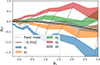 |
Fig. 13. Assembly bias in the Lagrangian bK2(b1) relation for halos split into four quartiles by spin (at fixed mass). All lines use the second-order spatial estimator and kd = 0.25 h Mpc−1 as damping scale. Dashed lines show the variation of b1 and bK2 at fixed mass. The bK2 − b1 relation shows a strong degree of assembly bias – with larger spin selections yielding larger bK2 and larger b1. |
The bK2 − b1 relation exhibits a strong degree of assembly bias with halo spin. For example, at b1 ∼ 1, the tidal bias of mass selected halos seems very small |bK2|≪0.1, but after the selection on halo spin, values may range between −1 and 0.5. In individual mass bins, the spin selection increases both the value of b1 and the value of bK2.
The sign, the b1 dependence, and the overall amplitude of the spin-assembly bias are all in good agreement with the measurements of Lazeyras et al. (2021). For example, at b1 = 2, we find assembly bias variations of ΔbK2 ∼ 2 (between low and high spins) consistent with their variations at  of around ΔbK2E ∼ 2 and the assembly bias decreases towards lower b1 and increases towards higher b1. Therefore, our measurements provide a validation of the results of that study, but it also shows that our method allows us to reliably measure the tidal bias.
While we do not present it here, we have also tested whether we can reproduce the concentration assembly bias that was measured by Lazeyras et al. (2021). We have found that if we also define concentration through vmax/v200c, then we find an assembly bias of a similar amplitude. However, if concentrations are defined through fits of the halo density profile, the assembly bias is smaller (possibly consistent with 0) and prefers the opposite sign. The concentration assembly bias seems therefore to be a bit more uncertain than that of the spin.
We conclude that even if bK2 seems quite small for mass selected halos, the tidal bias may not so easily be neglected for tracers that follow more general selection criteria. Values of the Lagrangian bK2 of an order of unity (and slightly larger) are a plausible possibility for realistic galaxy catalogues.
5.3. Biases of third derivative terms
In Figure 14, we show the measurements that we obtain by evaluating the bias estimators from Equations (140) and (141) and where we again divide by a factor of 2 to get b(∇δ)2 = bJ3 − 3/2, in accordance with the literature convention.
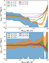 |
Fig. 14. Measurements of biases terms of third derivatives of the potential. The bias of the density gradient b(∇δ)2 (top) has a very strong scale dependence so that we cannot reliably measure it here. Bottom: Fully contracted third derivatives of the potential seem to have a very small associated bias parameter. |
The value of b(∇δ)2 appears to depend strongly on the damping scale and we cannot therefore claim a reliable measurement here. However, it seems mostly b(∇δ)2 < 0 which seems consistent with the idea that halos should preferentially form at peaks where density gradients should be small. However, at very large masses, b(∇δ)2 seems to become positive. We are not quite sure how to interpret this behaviour, but it might just be an artefact of the uncorrected scale dependencies. It is worth noting that the negative amplitude of b(∇δ)2 is quite significant b(∇δ)2 ∼ 10 h−2 Mpc2 and even grows towards larger scales. We therefore discuss whether this (usually neglected) bias term is worth including under some circumstances, as described late in this paper. We note that b(∇δ)2 was also measured by Biagetti et al. (2014). However, since we have not properly corrected the scale dependence here, we abstain from a comparison.
On the other hand, bJ3 ≡ 3 appears to be quite small, |bJ3 ≡ 3/2|≲5h−2Mpc2, for everything except the very high mass end. Therefore, the contributions of bJ3 ≡ 3 to the bias expansion should be significantly lower than b(∇δ)2.
6. Relevance of bias parameters
We aim to estimate the relevance of different contributions to the bias expansion. If we have a term of the form  of the re-normalised bias expansion, then we can estimate its relative relevance by comparing the typical difference in the predicted galaxy density field between a bias function, fX, which includes the term versus an expansion, f0, which neglects it, namely:
where the value of ⟨X2⟩ depends on the adopted damping scale and where σϵ, X is a dimensionless quantity that can be compared across different bias terms. For example, for the contribution of b3, we have
The value of σϵ, X quantifies the typical error that is made at the field level (in Lagrangian space) when neglecting the corresponding term.
We chose two halo sets M ∼ 1014 h−1 M⊙ and M ∼ 1015 h−1 M⊙ as examples and measured all their bias parameters with a damping scale of kd = 0.2 h Mpc−1 and used the second-order spatial estimators for all parameters (except b(∇δ)2 and b3 ≡ 3). We list the corresponding parameters in Table 2. The first set represents a moderately biased population, whereas the second set represents an example of strongly biased tracers. We then kepy these parameters fixed and evaluate ⟨X2⟩ at many different damping scales to obtain σϵ, X, which we show in Figure 15.
For the moderately biased tracers, the relevance of parameters decreases reasonably between different orders. However, this statement depends strongly on the considered damping scale. For instance, at kd = 0.4 h Mpc−1 many different terms reach similar amplitudes; whereas at kd = 0.05 h Mpc−1, there is a strong order of relevance among different terms. If we aim to fit a bias expansion at the field level at kd = 0.15 h Mpc−1 (marked as a vertical dotted line), then we would find that for the moderately biased set of b1 > b2 > b3 > b4, all of them lie within a factor of 2 of each other and for the strongly biased set, we even see their order has changed, namely, to: b2 > b1 > b4 > b3 and all of these lie within a factor of 3 of each other. This is certainly very problematic, since it does not at all seem clear that higher order terms are smaller than lower order terms here, which casts doubts on the convergence of the expansion. Of course this problem can be controlled by simply going to larger smoothing scales, but at the cost of a reduced constraining power. However, another possibility is to make use of the advantages of the cumulant bias parameters. With these parameters, significant parts of higher order terms get already absorbed by lower order parameters. For example, considering the first three terms of the bias expansion in terms of cumulant parameters:
Here β1 and β2 contribute also to the third term and to infinitely many higher order terms. If we write out the polynomial to high orders, but set β3 = 0, then the leading order error we would make is
which is identical to the error term from the canonical bias terms, but with a different fore-factor. Error estimates of these types are indicated as dashed lines in Figure 15. Strikingly, these are significantly smaller than the canonical terms and it seems now plausibly to reach good convergence at kd = 0.15 h Mpc−1. For instance, to reach σϵ ≤ 0.1 for the strongly biased set, we would only need to consider the terms (β1, β2, βL).
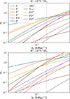 |
Fig. 15. Quantitative contribution of different bias terms to the bias expansion as a function of damping scale and for two different sets of tracers. To avoid cluttering, we omit the bias fore-factors of some terms in the legend. The vertical dotted line indicates an example scale of interest kd = 0.15 h Mpc−1. The dashed lines show the contributions of cumulant biases at orders of 3 and 4, which can directly be compared to the contributions of b3 and b4 (labelled as δ3 and δ4). |
It is noteworthy that the contribution of b(∇δ)2 is not much smaller than that of bL so that it might make sense to include this parameter more commonly in the bias expansion at scales kd ≳ 0.1 h Mpc−1. However, we remind the reader that there are some other possibly important parameters here that we have not considered, so that we cannot present a comprehensive picture of the relevance of bias parameters.
We conclude that it may have significant advantages to phrase the bias expansion in terms of the cumulant parameters, βn, instead of the canonical bias parameters. This is especially true when considering highly biased tracers or small smoothing scales, where the rate of convergence of the canonical expansion is excruciatingly slow.
7. Conclusions
In this article, we present a method for measuring bias parameters through moments of the galaxy environment distribution, p(δ|g). We have shown that such estimators can be derived both for scalar bias parameters such as b1 and bL and for tensorial ones such as bK2 and b(∇δ)2. Furthermore, we demonstrate that they can be made independent of scale if we consider spatial corrections at various orders. We have verified the reliability of these estimators by recovering well established relations between known parameters. Additionally, we used our estimators to measure terms that have been unknown thus far, such as b3 ≡ 3 and b(∇δ)2, where the latter appears to be particularly large so that it might be worth including it more commonly in the bias expansion.
The main benefits of the method are its simplicity and generality. We are only required to evaluate the linear field of a simulation at the Lagrangian locations of a set of tracers (e.g. given by the most bound id in a halo catalogue) and to take simple expectation values. This measurement uses a minimal number of discretisation steps, making it numerically robust and easy to understand. While a similar approach was previously used by Paranjape et al. (2013a,b), we have shown that it is possible to incorporate spatial corrections at any order to get accurate reconstructions of large-scale bias parameters, even at fairly large damping scales, kd. In contrast to measurement approaches that depend on forward models, for instance, of power spectra or correlation functions, measured bias parameters are significantly more independent of each other in the method at hand. For example, the measurement of b1 is completely independent of the assumed order of the expansion in powers of δ. This makes it generally unlikely that the parameters can numerically compensate for the absence of other terms. Finally, we note that all bias parameters can be evaluated at a low computational cost with a single simulation and that it is possible to use arbitrary filtering methods with the slight alterations explained in Appendix A.
However, to avoid confusion, we want to point out a few limitations of our method for estimating the biases. First of all, we note that our method assumes that the background distribution is known analytically. Therefore, it does not immediately translate to situations where this is not the case. For example, at third order in the bias expansion, time derivatives of the tidal tensor appear and these depend on the second Lagrangian perturbation theory potential, ϕ(2), which is not a Gaussian random field. Therefore, the formalism can only be translated to the associated bias parameters if the distribution of ϕ(2) and its derivatives can be written (or at least adequately approximated) analytically. Furthermore, the formalism cannot directly be applied to the Eulerian galaxy environment distribution pE(δ|g), since the non-linear Eulerian matter distribution pE(δ) does also not follow Gaussian statistics.
Beyond the novel bias estimators, we have also newly introduced the cumulant bias parameters
These cumulant bias parameters are proportional to the cumulants of the galaxy environement distribution8 and they are related to the canonical bias parameters exactly in the same way as cumulants relate to moments. When measuring these parameters, we found them to be more independent from each other than canonical bias parameters. Furthermore, we have shown that for halos cumulant biases of the order of n ≥ 3 are very close to zero. This has several intriguing consequences:
(1) The galaxy environment distribution and the bias function of halos are very well approximated by a Gaussian. This motivates the use of a Gaussian bias model for the order of n = 2, as well as alternative approaches, for instance, expanding around a Gaussian bias model for orders of n > 2. We will discuss the Gaussian bias model and its desirable properties in detail in a companion paper (Stücker et al. 2025).
(2) The co-evolution relations of halos of the order of n ≥ 3 are equivalent to βn = 0. Therefore, we may predict such relations between canonical bias parameters at very high orders by combining βn = 0 with the mapping between canonical and cumulant bias parameters. However, this also suggests that such co-evolution relations may not carry much physical significance, but instead they are the artefacts of a suboptimal basis choice. An expansion around a Gaussian model would naturally incorporate all of these relations at any order.
(3) The bias expansion may have significantly improved convergence when phrased in terms of cumulants instead of canonical bias parameters. At the field level, the convergence of the canonical expansion seems already questionable at scales of kd ≳ 0.15 h Mpc−1 since the parameters may easily rise as their order rises. However, when phrased in terms of cumulant biases, we expect neglected higher order terms to be significantly less important, as they are already well captured through lower order parameters.
Overall, we expect cumulant biases to be most beneficial whenever the canonical expansion shows poor convergence, for instance, at high masses, at late times, or at small smoothing scales.
The definitions we have given here should not be confused with those in works that consider the 2d joint distribution function of the smoothed galaxy density, ng, and the smoothed matter density, p(ng, δ), and their conditional p(ng|δ) (Dekel & Lahav 1999). Describing these is significantly more complicated, as they are two-dimensional and they contain stochastic contributions with a complicated dependence on two smoothing operations (for defining the matter contrast and the galaxy density, respectively).
Corresponding to a sharp truncation scale in Fourier space, as explained in Sect. 3.2.
Acknowledgments
The authors thank Simon White, Oliver Hahn and Fabian Schmidt for helpful discussions and comments to the draft. JS thanks Oliver Philcox for helpful discussions. We acknowledge funding from the Spanish Ministry of Science and Innovation through grant number PID2021-128338NB-I00. RV acknowledges the support of the Juan de la Cierva fellowship (FJC2021-048002-I). MPI is supported by STFC consolidated grant no. RA5496.
References
- Abidi, M. M., & Baldauf, T. 2018, JCAP, 2018, 029 [CrossRef] [Google Scholar]
- Akitsu, K., Li, Y., & Okumura, T. 2021, JCAP, 2021, 041 [CrossRef] [Google Scholar]
- Alam, S., Aubert, M., Avila, S., et al. 2021, Phys. Rev. D, 103, 083533 [NASA ADS] [CrossRef] [Google Scholar]
- Amendola, L., Appleby, S., Avgoustidis, A., et al. 2018, Liv. Rev. Rel., 21, 2 [Google Scholar]
- Angulo, R. E., & Hahn, O. 2022, Liv. Rev. Comput. Astrophys., 8, 1 [CrossRef] [Google Scholar]
- Angulo, R. E., Zennaro, M., Contreras, S., et al. 2021, MNRAS, 507, 5869 [NASA ADS] [CrossRef] [Google Scholar]
- Baldauf, T., Desjacques, V., & Seljak, U. 2015, Phys. Rev. D, 92, 123507 [Google Scholar]
- Baldauf, T., Mirbabayi, M., Simonović, M., & Zaldarriaga, M. 2016a, arXiv e-prints [arXiv:1602.00674] [Google Scholar]
- Baldauf, T., Seljak, U., Senatore, L., & Zaldarriaga, M. 2016b, JCAP, 2016, 007 [NASA ADS] [CrossRef] [Google Scholar]
- Bardeen, J. M., Bond, J. R., Kaiser, N., & Szalay, A. S. 1986, ApJ, 304, 15 [Google Scholar]
- Barreira, A. 2020, JCAP, 2020, 031 [CrossRef] [Google Scholar]
- Barreira, A., Lazeyras, T., & Schmidt, F. 2021, JCAP, 2021, 029 [CrossRef] [Google Scholar]
- Baumann, D., Nicolis, A., Senatore, L., & Zaldarriaga, M. 2012, JCAP, 2012, 051 [Google Scholar]
- Berlind, A. A., & Weinberg, D. H. 2002, ApJ, 575, 587 [Google Scholar]
- Bernardeau, F., Colombi, S., Gaztañaga, E., & Scoccimarro, R. 2002, Phys. Rep., 367, 1 [Google Scholar]
- Biagetti, M., Chan, K. C., Desjacques, V., & Paranjape, A. 2014, MNRAS, 441, 1457 [Google Scholar]
- Bullock, J. S., Dekel, A., Kolatt, T. S., et al. 2001, ApJ, 555, 240 [NASA ADS] [CrossRef] [Google Scholar]
- Cacciato, M., Lahav, O., van den Bosch, F. C., Hoekstra, H., & Dekel, A. 2012, MNRAS, 426, 566 [Google Scholar]
- Chaves-Montero, J., Angulo, R. E., Schaye, J., et al. 2016, MNRAS, 460, 3100 [NASA ADS] [CrossRef] [Google Scholar]
- Chaves-Montero, J., Angulo, R. E., & Contreras, S. 2023, MNRAS, 521, 937 [Google Scholar]
- Chen, S.-F., Vlah, Z., & White, M. 2020, JCAP, 2020, 062 [CrossRef] [Google Scholar]
- Colas, T., d’Amico, G., Senatore, L., Zhang, P., & Beutler, F. 2020, JCAP, 2020, 001 [Google Scholar]
- Conroy, C., Wechsler, R. H., & Kravtsov, A. V. 2006, ApJ, 647, 201 [Google Scholar]
- Contreras, S., Angulo, R. E., & Zennaro, M. 2021, MNRAS, 508, 175 [NASA ADS] [CrossRef] [Google Scholar]
- Contreras, S., Chaves-Montero, J., & Angulo, R. E. 2023, MNRAS, 525, 3149 [NASA ADS] [CrossRef] [Google Scholar]
- Croton, D. J., Gao, L., & White, S. D. M. 2007, MNRAS, 374, 1303 [Google Scholar]
- Croton, D. J., Stevens, A. R. H., Tonini, C., et al. 2016, ApJS, 222, 22 [Google Scholar]
- Dalal, N., White, M., Bond, J. R., & Shirokov, A. 2008, ApJ, 687, 12 [NASA ADS] [CrossRef] [Google Scholar]
- d’Amico, G., Gleyzes, J., Kokron, N., et al. 2020, JCAP, 2020, 005 [Google Scholar]
- Davé, R., Anglés-Alcázar, D., Narayanan, D., et al. 2019, MNRAS, 486, 2827 [Google Scholar]
- Dekel, A., & Lahav, O. 1999, ApJ, 520, 24 [Google Scholar]
- DeRose, J., Kokron, N., Banerjee, A., et al. 2023, JCAP, 2023, 054 [CrossRef] [Google Scholar]
- Desjacques, V., Crocce, M., Scoccimarro, R., & Sheth, R. K. 2010, Phys. Rev. D, 82, 103529 [CrossRef] [Google Scholar]
- Desjacques, V., Jeong, D., & Schmidt, F. 2018, Phys. Rep., 733, 1 [Google Scholar]
- Dragomir, R., Rodríguez-Puebla, A., Primack, J. R., & Lee, C. T. 2018, MNRAS, 476, 741 [NASA ADS] [CrossRef] [Google Scholar]
- Dubois, Y., Pichon, C., Welker, C., et al. 2014, MNRAS, 444, 1453 [Google Scholar]
- Faltenbacher, A., & White, S. D. M. 2010, ApJ, 708, 469 [NASA ADS] [CrossRef] [Google Scholar]
- Ferreras, I., Hopkins, A. M., Lagos, C., et al. 2019, MNRAS, 487, 435 [Google Scholar]
- Frenk, C. S., White, S. D. M., Davis, M., & Efstathiou, G. 1988, ApJ, 327, 507 [NASA ADS] [CrossRef] [Google Scholar]
- Gao, L., & White, S. D. M. 2007, MNRAS, 377, L5 [NASA ADS] [CrossRef] [Google Scholar]
- Gao, L., Springel, V., & White, S. D. M. 2005, MNRAS, 363, L66 [NASA ADS] [CrossRef] [Google Scholar]
- Genel, S., Bryan, G. L., Springel, V., et al. 2019, ApJ, 871, 21 [NASA ADS] [CrossRef] [Google Scholar]
- Henriques, B. M. B., White, S. D. M., Thomas, P. A., et al. 2015, MNRAS, 451, 2663 [Google Scholar]
- Ivanov, M. M., Simonović, M., & Zaldarriaga, M. 2020, JCAP, 2020, 042 [Google Scholar]
- Kaiser, N. 1984, ApJ, 284, L9 [NASA ADS] [CrossRef] [Google Scholar]
- Kauffmann, G., Colberg, J. M., Diaferio, A., & White, S. D. M. 1999, MNRAS, 303, 188 [NASA ADS] [CrossRef] [Google Scholar]
- Kokron, N., DeRose, J., Chen, S.-F., White, M., & Wechsler, R. H. 2021, MNRAS, 505, 1422 [NASA ADS] [CrossRef] [Google Scholar]
- Lacey, C. G., Baugh, C. M., Frenk, C. S., et al. 2016, MNRAS, 462, 3854 [Google Scholar]
- Lagos, C. d. P., Tobar, R. J., Robotham, A. S. G., et al. 2018, MNRAS, 481, 3573 [CrossRef] [Google Scholar]
- Lazeyras, T., & Schmidt, F. 2018, JCAP, 2018, 008 [CrossRef] [Google Scholar]
- Lazeyras, T., & Schmidt, F. 2019, JCAP, 2019, 041 [Google Scholar]
- Lazeyras, T., Wagner, C., Baldauf, T., & Schmidt, F. 2016, JCAP, 2016, 018 [CrossRef] [Google Scholar]
- Lazeyras, T., Barreira, A., & Schmidt, F. 2021, JCAP, 2021, 063 [CrossRef] [Google Scholar]
- Lehmann, B. V., Mao, Y.-Y., Becker, M. R., Skillman, S. W., & Wechsler, R. H. 2017, ApJ, 834, 37 [NASA ADS] [CrossRef] [Google Scholar]
- Levi, M., Bebek, C., Beers, T., et al. 2013, arXiv e-prints [arXiv:1308.0847] [Google Scholar]
- Li, Y., Hu, W., & Takada, M. 2014, Phys. Rev. D, 89, 083519 [NASA ADS] [CrossRef] [Google Scholar]
- Lukacs, E. 1970, Characteristic Functions, 2nd edn. (Griffin) [Google Scholar]
- Masaki, S., Nishimichi, T., & Takada, M. 2020, MNRAS, 496, 483 [NASA ADS] [CrossRef] [Google Scholar]
- Meurer, A., Smith, C. P., Paprocki, M., et al. 2017, PeerJ Comput. Sci., 3 [Google Scholar]
- Mo, H. J., & White, S. D. M. 1996, MNRAS, 282, 347 [Google Scholar]
- Modi, C., Castorina, E., & Seljak, U. 2017, MNRAS, 472, 3959 [Google Scholar]
- Modi, C., Chen, S.-F., & White, M. 2020, MNRAS, 492, 5754 [NASA ADS] [CrossRef] [Google Scholar]
- Montero-Dorta, A. D., Pérez, E., Prada, F., et al. 2017, ApJ, 848, L2 [NASA ADS] [CrossRef] [Google Scholar]
- Musso, M., Paranjape, A., & Sheth, R. K. 2012, MNRAS, 427, 3145 [CrossRef] [Google Scholar]
- Nishimichi, T., D’Amico, G., Ivanov, M. M., et al. 2020, Phys. Rev. D, 102, 123541 [NASA ADS] [CrossRef] [Google Scholar]
- Ortega-Martinez, S., Contreras, S., & Angulo, R. 2024, A&A, 689, A66 [NASA ADS] [CrossRef] [EDP Sciences] [Google Scholar]
- Paranjape, A., & Sheth, R. K. 2012, MNRAS, 426, 2789 [Google Scholar]
- Paranjape, A., Sefusatti, E., Chan, K. C., et al. 2013a, MNRAS, 436, 449 [CrossRef] [Google Scholar]
- Paranjape, A., Sheth, R. K., & Desjacques, V. 2013b, MNRAS, 431, 1503 [CrossRef] [Google Scholar]
- Paranjape, A., Hahn, O., & Sheth, R. K. 2018, MNRAS, 476, 3631 [NASA ADS] [CrossRef] [Google Scholar]
- Peacock, J. A., & Smith, R. E. 2000, MNRAS, 318, 1144 [Google Scholar]
- Pellejero Ibañez, M., Stücker, J., Angulo, R. E., et al. 2022, MNRAS, 514, 3993 [Google Scholar]
- Pellejero Ibañez, M., Angulo, R. E., Zennaro, M., et al. 2023, MNRAS, 520, 3725 [Google Scholar]
- Philcox, O. H. E., & Ivanov, M. M. 2022, Phys. Rev. D, 105, 043517 [CrossRef] [Google Scholar]
- Planck Collaboration VI. 2020, A&A, 641, A6 [NASA ADS] [CrossRef] [EDP Sciences] [Google Scholar]
- Reddick, R. M., Wechsler, R. H., Tinker, J. L., & Behroozi, P. S. 2013, ApJ, 771, 30 [Google Scholar]
- Salcedo, A. N., Weinberg, D. H., Wu, H.-Y., & Wibking, B. D. 2022a, MNRAS, 510, 5376 [CrossRef] [Google Scholar]
- Salcedo, A. N., Zu, Y., Zhang, Y., et al. 2022b, Sci. China Phys. Mech. Astron., 65, 109811 [Google Scholar]
- Sato-Polito, G., Montero-Dorta, A. D., Abramo, L. R., Prada, F., & Klypin, A. 2019, MNRAS, 487, 1570 [NASA ADS] [CrossRef] [Google Scholar]
- Schaye, J., Crain, R. A., Bower, R. G., et al. 2015, MNRAS, 446, 521 [Google Scholar]
- Sheth, R. K., Chan, K. C., & Scoccimarro, R. 2013, Phys. Rev. D, 87, 083002 [NASA ADS] [CrossRef] [Google Scholar]
- Springel, V., White, S. D. M., Tormen, G., & Kauffmann, G. 2001, MNRAS, 328, 726 [Google Scholar]
- Stevens, A. R. H., Croton, D. J., & Mutch, S. J. 2016, MNRAS, 461, 859 [Google Scholar]
- Stücker, J., Schmidt, A. S., White, S. D. M., Schmidt, F., & Hahn, O. 2021, MNRAS, 503, 1473 [CrossRef] [Google Scholar]
- Stücker, J., Pellejero-Ibáñez, M., Voivodic, R., & Angulo, R. E. 2025, A&A, 694, A29 [NASA ADS] [CrossRef] [EDP Sciences] [Google Scholar]
- Szalay, A. S. 1988, ApJ, 333, 21 [NASA ADS] [CrossRef] [Google Scholar]
- Tinker, J. L., Robertson, B. E., Kravtsov, A. V., et al. 2010, ApJ, 724, 878 [NASA ADS] [CrossRef] [Google Scholar]
- Tucci, B., Montero-Dorta, A. D., Abramo, L. R., Sato-Polito, G., & Artale, M. C. 2021, MNRAS, 500, 2777 [Google Scholar]
- Villaescusa-Navarro, F., Anglés-Alcázar, D., Genel, S., et al. 2021, ApJ, 915, 71 [NASA ADS] [CrossRef] [Google Scholar]
- Vlah, Z., Castorina, E., & White, M. 2016, JCAP, 2016, 007 [Google Scholar]
- Vogelsberger, M., Genel, S., Springel, V., et al. 2014, MNRAS, 444, 1518 [Google Scholar]
- Wagner, C., Schmidt, F., Chiang, C. T., & Komatsu, E. 2015, MNRAS, 448, L11 [CrossRef] [Google Scholar]
- Wechsler, R. H., Zentner, A. R., Bullock, J. S., Kravtsov, A. V., & Allgood, B. 2006, ApJ, 652, 71 [NASA ADS] [CrossRef] [Google Scholar]
- White, S. D. M. 1979, MNRAS, 186, 145 [NASA ADS] [CrossRef] [Google Scholar]
- White, S. D. M. 1984, ApJ, 286, 38 [NASA ADS] [CrossRef] [Google Scholar]
- Zehavi, I., Contreras, S., Padilla, N., et al. 2018, ApJ, 853, 84 [NASA ADS] [CrossRef] [Google Scholar]
- Zennaro, M., Angulo, R. E., Contreras, S., Pellejero-Ibáñez, M., & Maion, F. 2022, MNRAS, 514, 5443 [NASA ADS] [CrossRef] [Google Scholar]
- Zennaro, M., Angulo, R. E., Pellejero-Ibáñez, M., et al. 2023, MNRAS, 524, 2407 [Google Scholar]
- Zheng, Z., Berlind, A. A., Weinberg, D. H., et al. 2005, ApJ, 633, 791 [NASA ADS] [CrossRef] [Google Scholar]
Appendix A: Estimators with different filters
In Section 2, we have shown derivations under the assumption of a sharp k-space filter. For this choice all considered bias functions and bias parameters relate trivially to the separate-universe parameters that are commonly referred to in the literature. However, in general other filtering kernels could also be chosen. For example if we define the smoothed density as
where δl is the smoothed density and δ the unsmoothed one. If the filter W is for example chosen to be a Gaussian kernel,
instead of a sharp k filter, then some considerations have to be adapted. In principle, all of the formula from Section 2 could still be applied, but they would refer to a different set of bias parameters that describe the response to perturbations of a different shape. Rather than introducing a new set of bias parameters, it is more convenient to directly write the commonly used parameters in terms of the new basis. Therefore, we show here how to directly measure the separate-universe bias parameters from the moments of the galaxy environment distribution that was obtained with a density field that was filtered with any kernel.
First of all, we consider how a bias function on very large scales fl(δl) should relate to the bias function on some much smaller scale fs(δs). If the PBS is still valid on the smaller scale, then the probability of forming a galaxy, given knowledge of δs and δl depends only on the value of δs:
Under this assumption, we can re-express the large scale bias function through the small scale function marginalised over the conditional probability of the small scale densities:
Since, the joint distribution of δs and δl is a multivariate Gaussian, the conditional distribution corresponds to a multivariate Gaussian that is conditioned on the value of one variable, which itself is a Gaussian with modified mean and covariance:


where α = σls2/σll2 corresponds to the correlation between the smoothed large-scale and small-scale density fields, σll2 = ⟨δlδl⟩, σls2 = ⟨δlδs⟩ and σss = ⟨δsδs⟩.
If we define the re-normalised bias function, Fα, through the bias function fl as in Section 2, then we find
where pss is simply the background distribution of the small scale densities. This can be shown either by evaluating the integrals (corresponding to convolutions) explicitly or by considering the large scale limit of fl where σ* → σss.
We can now relate the re-normalised bias functions obtained with different filtering methods, since we may assume that fs is independent of the filter employed on large scales. Therefore,
where we have indicated the usage of different filters through different α in the index. Therefore, different filters simply lead to a rescaling of the re-normalised bias function. The value of α depends on the filter and the smoothing scale. If we assume that δs was obtained with some small scale filter Ws and δl with Wl, we have
where the last approximation assumes that Ws is very close to 1 over the support of Wl, because Wl corresponds to a much larger scale smoothing than Ws. Furthermore, we have

It is easy to see that α = 1 for any sharp Fourier space filter, independent of the filtering scale. However, for other filters it is important to note that α may be generally larger than 1, for example α ∼ 2 for a Gaussian filter at scales of kd ∼ 0.1 h Mpc−1. Furthermore, α depends generally on the filtering-scale. The re-normalised bias function does therefore only correspond to a well-defined limit at arbitrary large scales if α is constant (as for the sharp k filter).
Since the case α = 1 seems clearly to be the simplest and leads to a sensibly scale-independent re-normalisation, we consider it as the reference case and simply label its re-normalised bias function F, and we have focused in the main-text on the discussion of this case. However, we can still use the relations derived in the main-text to measure the properties of F directly through measuring aspects of some filter-dependent function Fα.
We directly show this for the general multivariate case here by adapting the considerations from Section 2.7. For the multivariate case the re-normalised bias functions are relate as
where

where Cls may more conveniently be measured as ⟨xm⊗xm⟩, where xm is evaluated in the linear fields filtered with  .
.
The cumulant-generating function of the galaxy environment distribution with δl is again given through Equation (64), just with FA instead of F:
For measuring the cumulant bias parameters, we may then define a more convenient variable,

which has the cumulant generating function,
Thus, the cumulant bias parameters can be inferred by differentiating, leading to:
where  . We can therefore measure the separate-universe bias parameters with an arbitrarily filtered distribution in a very similar manner to the one using a sharp k-space filter. It is worth noting that the inferred relations show also an important property: If βn vanish for n > 2, which automatically implies that the corresponding cumulants vanish for any filtered galaxy environment distribution. Therefore, if the bias function is Gaussian for one filter, then it will also appear Gaussian for any other filter.
Appendix B: Isotropic tensors
B.1. Tensors with three or more symmetry groups
In the main text, we limit our discussion to an explanation of how to obtain basis tensors for tensor spaces with at most two symmetry groups. However, for higher order biases, for instance, the equivalent of b3 the isotropic tensor decomposition requires consideration of additional symmetries. We define 𝕍222 as the space of tensors that are symmetric under permutations of the first two, second two and third two indices. Furthermore, we define 𝕍(222) as the space of tensors that are additionally invariant to exchanges of these symmetry groups. These spaces have different number of basis tensors,


where
is additionally symmetrised between exchanges between the symmetry groups and the other tensors are given by


The basis tensors of 𝕍(222) are visualised through a diagram in Figure B.1. The third derivative tensor of that would appear in the bias expansion can be decomposed in this space
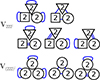 |
Fig. B.1. Illustration of the basis tensors of 𝕍222 versus those of 𝕍(222). Top: without the symmetry requirement between groups (indicated by usage of different symbols for each group) there are five basis tensors. Bottom: With the additional symmetry requirement between groups (indicated by usage of the same symbol for each group), since the latter three tensors of 𝕍222 get all united to a single symmetrised term (bottom). |
B.2. Covariance of potential derivatives
To find an explicit form for the distribution of the derivatives of the tidal tensor and other higher order derivatives of the potential, we need to find their covariance matrix and invert it.
For this we first consider the covariance between any derivatives of the potential. This is given by
where δk is the Fourier transform of density field δ and we have used that δ is a real field so that δk(k) = δk*(−k). Using the definition of the power spectrum,

where δD is the Dirac delta function, we can simplify
We can see that this expression does not depend on the order of the indices, nor whether they stem from the first or the second potential term. Therefore, we just count the total number n1 of occurrences of kx, n2 of ky and n3 of kz. Without loss of generality we can order the coordinates, such that n1 ≥ n2 ≥ n3. Furthermore, we can switch to spherical coordinates and replace the cosine of the azimutal variable:
so that we have
These integrals can easily be evaluated by hand or with a computer algebra system. We list a few examples of the covariances in Table B.1 We note that only terms where each n1, n2, and n3 are even are non-zero. We note that all uneven terms are zero, so that, for instance, the two-second derivatives of the potential have zero covariance with the third derivatives, but a non-zero covariance with the fourth derivatives.
Covariances of various derivatives of the potential.
B.3. The distribution of the tidal tensor
From Equation (B.12) it can be seen that the covariance tensor of any derivatives of the potential has to be an isotropic tensor with full symmetry in all indices. Therefore, the covariance matrix of the tidal tensor is CT ∈ 𝕍4 so that it has to be proportional to I4 with a coefficient that we can read off from table B.1:

This tensor is not invertible, since, for instance, the T12 component is perfectly degenerate with the T21 component. However, in such cases where the distribution of T can still be inferred by constructing a generalised inverse  , which has the following property:

It then holds that
To find the generalised inverse we may assume that CT+ ∈ 𝕍22, so that we can make the Ansatz
We can use the decomposition  (determined computationally) and evaluate Equation (B.18) term by term:
where we have evaluated the appearing tensor products computationally. By identifying coefficients, we find  and
and  and therefore we have the generalised inverse of the covariance matrix:
and the distribution of the tidal tensor is given by
B.4. The distribution of third derivatives
The third derivative tensor of the potential S has the covariance matrix

Analogously to the calculation in Section B.3, we find the generalised inverse
where we have again used numerical representations to evaluate products between isotropic tensors when evaluating Equation (B.18). Therefore, the distribution of S is given by
where in the last line we have defined some new scalar variables through the given contractions, where S3 − 3 = (∇δ)2.
B.5. Joint distribution of second and fourth derivatives
We can write the covariance matrix of fourth and second derivatives as a block matrix
For its inverse, we make the Ansatz
and we find the solution to its generalised inverse by solving
with a computer algebra system and find
![$$ \begin{aligned} \mathsf C _\mathsf{T \mathsf R }^+= \left[\begin{matrix}\frac{15 \sigma _{2}^{2} \mathsf J _{2 = 2}}{2 \sigma _{0}^{2} \sigma _{2}^{2} - 2 \sigma _{1}^{4}} + \frac{\sigma _{2}^{2} \mathsf J _{22}}{\sigma _{0}^{2} \sigma _{2}^{2} - \sigma _{1}^{4}}&- \frac{15 \sigma _{1}^{2} \mathsf J _{2 = 4}}{2 \sigma _{0}^{2} \sigma _{2}^{2} - 2 \sigma _{1}^{4}} - \frac{\sigma _{1}^{2} \mathsf J _{24}}{\sigma _{0}^{2} \sigma _{2}^{2} - \sigma _{1}^{4}}\\ \frac{15 \sigma _{1}^{2} \mathsf J _{4 = 2}}{2 \sigma _{0}^{2} \sigma _{2}^{2} - 2 \sigma _{1}^{4}} - \frac{\sigma _{1}^{2} \mathsf J _{42}}{\sigma _{0}^{2} \sigma _{2}^{2} - \sigma _{1}^{4}}&\frac{15 \sigma _{0}^{2} \mathsf J _{4 = 4}}{2 \sigma _{0}^{2} \sigma _{2}^{2} - 2 \sigma _{1}^{4}} + \frac{\sigma _{0}^{2} \mathsf J _{44}}{\sigma _{0}^{2} \sigma _{2}^{2} - \sigma _{1}^{4}} + \frac{315 \mathsf J _{4= = 4}}{8 \sigma _{2}^{2}}\end{matrix}\right]. \end{aligned} $$](/articles/aa/full_html/2025/07/aa51176-24/aa51176-24-eq254.gif)
The joint distribution of second and fourth derivatives of the potential can be written as
B.6. Tidal estimator with spatial correction
We find the tidal estimator with spatial corrections of the order of 2 as:
where

While we do not list them here, we have verified that if we analogously evaluate the expressions for bJ2, bJ4, bJ22 and bJ24 that they are identical to the estimators for b1, bL, b2, and bδ, L, respectively, from Equations (49) - (53).
All Tables
All Figures
|
Fig. 1. Illustration of the inference of the halo environment distribution p(δ|g). Left: Galaxies traced back to their origin in Lagrangian space (marked as black dots) and with the (smoothed) linear density field, δ, inferred at their Lagrangian locations. Right: Environment distribution (orange histogram) given by the distribution of δ at the galaxy locations which is notably biased relative to the matter distribution, p(δ), (blue histogram and a Gaussian represented as dashed line). The galaxy environment distribution is well approximated through p(δ)f(δ), where here f(δ) is a quadratic polynomial bias function. |
| In the text | |
|
Fig. 2. b1 as a function of halo mass using the estimators from Equation (15) at the top and Equation (49) at the bottom, measured at different damping scales (different coloured regions). The shaded regions indicate the 1σ certainty region of the estimators. Using the b1 estimator that includes the Laplacian correction increases the uncertainty of the b1 estimates, but reduces the dependence on the damping scale, leading to a good agreement across different scales. |
| In the text | |
|
Fig. 3. Scale dependence of the error in b1 estimates for different halo mass selections. The error is expressed relatively to the measurement with spatial order of 2 at |
| In the text | |
|
Fig. 4. b2 and β2 as a function of b1 = β1 using the second-order spatial estimators. The black dashed line is the b2(b1) relation inferred by Lazeyras et al. (2016) from separate-universe simulations. The second-order spatial estimators seem consistent with the literature co-evolution relation down to damping scales of kd ∼ 0.15 − 0.2 h Mpc−1. It is noteworthy that β2 < 0 appears to always hold, which means that the width of the galaxy environment distribution p(δ|g) is always smaller than that of the background p(δ). Therefore, the cumulant bias parameter β2 − β1 relation appears slightly simpler than the b2 − b1 relation. |
| In the text | |
|
Fig. 5. Uncertainty of b2 measurements (solid lines) and β2 measurements (dashed lines) as a function of b1 for different damping scales. The uncertainty of β2 is significantly smaller than of b2 for high values of b1. |
| In the text | |
|
Fig. 6. Correlation coefficient α12 between the b1 and b2 measurement (solid) and the β1 and β2 measurement (dashed). Note: β2 as a parameter is much more independent of the value of b1 than b2. |
| In the text | |
|
Fig. 7. Co-evolution relations of higher order bias parameters b3 and β3 (top) and b4 and β4 (bottom) for the second-order spatial bias estimators. For b4 we indicate as a dashed line a prediction that follows from combining the Lazeyras et al. (2016) measurements of b1, b2 and b3 with Equation (30) when using β4 = 0. Strikingly, β3 and β4 are extremely close to 0 – independently of the value of b1. |
| In the text | |
|
Fig. 8. Lagrangian Laplacian bias bL as a function of halo mass. At masses M ≲ 3 × 10¹³ h−1 M⊙ the scale dependence of the bL measurements disappears and they agree well with the fits of the Eulerian Laplacian bias from Lazeyras & Schmidt (2019). |
| In the text | |
|
Fig. 9. Maximum damping scale where the PBS can be valid and bias scale-independent. The three reddish contours show the break-down scale of density-only bias models, estimated with bias parameters measured at different scales, and the three green-blueish contours show it for (δ, L) bias models. The black dashed line shows the wavenumber associated with the Lagrangian radius of halos. The break-down scale is consistent across different measurements and only seems to scale strongly with halo radius for the (δ) case. |
| In the text | |
|
Fig. 10. Graphic representation of the isotropic tensors that form a basis for a few selected isotropic tensor spaces with symmetries. All basis tensors of a space with given symmetry can be constructed by considering the number of different ways that the symmetry groups can be connected. In this figure each circle with number n represents a group of n fully symmetric indices and each connection represents one delta symbol (that can either connect two indices from the same group or from two different groups). |
| In the text | |
|
Fig. 11. Tidal bias as a function of mass and for different damping scales measured with the zeroth-order spatial estimator (top) versus the second-order spatial estimator (bottom). The second-order spatial estimator exhibits significantly reduced scale dependence at the price of increased error bars. |
| In the text | |
|
Fig. 12. Co-evolution relation bK2 versus b1. Coloured shaded regions are our measurements and error bars show the measurements from Lazeyras & Schmidt (2018). Black lines include measurements from Zennaro et al. (2022), Modi et al. (2017) and Abidi & Baldauf (2018), an excursion set prediction from Sheth et al. (2013) and an approximation that we propose as bK2 = −0.05b12. |
| In the text | |
|
Fig. 13. Assembly bias in the Lagrangian bK2(b1) relation for halos split into four quartiles by spin (at fixed mass). All lines use the second-order spatial estimator and kd = 0.25 h Mpc−1 as damping scale. Dashed lines show the variation of b1 and bK2 at fixed mass. The bK2 − b1 relation shows a strong degree of assembly bias – with larger spin selections yielding larger bK2 and larger b1. |
| In the text | |
|
Fig. 14. Measurements of biases terms of third derivatives of the potential. The bias of the density gradient b(∇δ)2 (top) has a very strong scale dependence so that we cannot reliably measure it here. Bottom: Fully contracted third derivatives of the potential seem to have a very small associated bias parameter. |
| In the text | |
|
Fig. 15. Quantitative contribution of different bias terms to the bias expansion as a function of damping scale and for two different sets of tracers. To avoid cluttering, we omit the bias fore-factors of some terms in the legend. The vertical dotted line indicates an example scale of interest kd = 0.15 h Mpc−1. The dashed lines show the contributions of cumulant biases at orders of 3 and 4, which can directly be compared to the contributions of b3 and b4 (labelled as δ3 and δ4). |
| In the text | |
|
Fig. B.1. Illustration of the basis tensors of 𝕍222 versus those of 𝕍(222). Top: without the symmetry requirement between groups (indicated by usage of different symbols for each group) there are five basis tensors. Bottom: With the additional symmetry requirement between groups (indicated by usage of the same symbol for each group), since the latter three tensors of 𝕍222 get all united to a single symmetrised term (bottom). |
| In the text | |
Current usage metrics show cumulative count of Article Views (full-text article views including HTML views, PDF and ePub downloads, according to the available data) and Abstracts Views on Vision4Press platform.
Data correspond to usage on the plateform after 2015. The current usage metrics is available 48-96 hours after online publication and is updated daily on week days.
Initial download of the metrics may take a while.