| Issue |
A&A
Volume 699, July 2025
|
|
|---|---|---|
| Article Number | A52 | |
| Number of page(s) | 12 | |
| Section | Catalogs and data | |
| DOI | https://doi.org/10.1051/0004-6361/202450972 | |
| Published online | 27 June 2025 | |
Identification of quasars that are variable over long timescales from infrared surveys
Ensemble variability and structure function properties
1
Department of Astronomy, Faculty of Physics, University of Sofia,
1164
Sofia,
Bulgaria
2
European Southern Observatory,
Karl-Schwarzschild-Str. 2,
85748
Garching bei München,
Germany
★ Corresponding authors: This email address is being protected from spambots. You need JavaScript enabled to view it.
; This email address is being protected from spambots. You need JavaScript enabled to view it.
Received:
3
June
2024
Accepted:
22
April
2025
Abstract
Context. Quasars are variable, and their variability can both constrain their physical properties and help to identify them.
Aims. We aim to look for ways to efficiently identify quasars exhibiting consistent variability over multi-year timescales based on a small number of epochs. Using infrared (IR) is desirable to avoid bias against reddened objects.
Methods. We compared the apparent brightness of known quasars that have been observed with two IR surveys, covering up to a twenty-year baseline: the Two Micron All Sky Survey (2MASS; 1997-2001) and the VISTA Hemisphere Survey (VHS; 2009-2017). We looked at the previous studies of the selected variable quasars to see if their variable behaviour is known, and when available we used multi-epoch monitoring with the Zwicky Transient Facility (ZTF) to obtain a measure of optical variability of individual objects.
Results. We built a sample of nearly 2500 quasars that show statistically significant variability between the 2MASS and VHS. About 1500 of these come from the new Quaia sample based on Gaia spectra, and about 1/3 of these have hardly been studied. The Quaia sample constitutes the main product of this work. Based on ensemble variability and structure function analysis, we demonstrate that the selected objects in our sample are representative of the typical quasar population and show behaviour consistent with other quasar samples. Our analysis strengthens previous results showing, e.g., that variability decreases with the rest-frame wavelength and that it exhibits peaks for certain absolute magnitudes of the quasars. Similarly, the structure function shows an increase in variability for rest-frame time lags below ∼1500 d and a decrease for longer lags, just as in previous studies.
Conclusions. Our selection, even though it is based on two epochs only, seems to be surprisingly robust, showing up to ∼11% contamination by quasars that show stable non-variable behaviour in the ZTF.
Key words: catalogs / galaxies: active / quasars: general
© The Authors 2025
 Open Access article, published by EDP Sciences, under the terms of the Creative Commons Attribution License (https://creativecommons.org/licenses/by/4.0), which permits unrestricted use, distribution, and reproduction in any medium, provided the original work is properly cited.
This article is published in open access under the Subscribe to Open model. This email address is being protected from spambots. You need JavaScript enabled to view it. to support open access publication.
1 Introduction
Quasi-stellar objects (QSO) or quasars are powerful and distant active galactic nuclei (AGNs) that were identified in the early 1960s (Greenstein 1963; Oke 1963; Schmidt 1963). Some of the early quasars were well known to vary on short timescales, which implied a compact structure including a central continuum source surrounded by an emission-line region (Matthews & Sandage 1963; Smith & Hoffleit 1963). Soon accreting supermassive black holes were proposed as quasars’ energy sources (Hoyle & Fowler 1963a,b; Salpeter 1964). Subsequent monitoring demonstrated that the compact nature of the black holes agreed well with the observed variability timescales (Smith & Hoffleit 1961, 1963; Angione 1973; Blandford & McKee 1982; Hook et al. 1994; Trevese et al. 1994). Antonucci & Miller (1985) and Antonucci (1993) organised the rich observational results of the preceding decades into the unified model of active galaxies that is commonly accepted today.
The variability proved to be a useful tool in at least two aspects - putting observational constraints on the spatial structure of their inner regions and to measure the masses of the central black holes (Blandford & McKee 1982; Peterson 1993; Peterson et al. 2004), and helping to identify QSOs from their variability patterns in large synoptic sky surveys (Hawkins & Véron 1990; Trevese et al. 2008; Schmidt et al. 2010). Lira (2021) summarized the recent understanding of QSO variability studies.
Previous optical long-term variability studies (e.g. de Vries et al. 2003, 2005) indicated the following:
quasars are more variable towards the blue than towards the red
variability increases monotonically with increasing time lag - less luminous quasars are more variable than more luminous ones
blazars tend to be more variable than other quasars
Various variability mechanisms have been discussed: thermal instabilities in the accretion disc (Shakura & Sunyaev 1976), circumnuclear starburst or accretion instability (Kawaguchi et al. 1998), and the interaction between a complex, multi-structured accretion disc (Haardt & Maraschi 1991), among others.
The need to create complete samples of variable quasars became obvious early on (e.g. Hawkins 1983), because they would give a glimpse of quasars as a population and because large samples would hopefully include rare objects that have always been useful in identifying and characterising the most extreme physical processes responsible for the variability.
Reliably detected variable quasar samples have multiple applications. One of the most obvious is finding binary black holes - a process that gives us a direct glimpse into the late stages of galaxy merging and the growth of supermassive black holes and the bulges that they are immersed in. Chen et al. (2020) reported a 20-year optical monitoring. Their light curves demonstrate the two major obstacles to this goal: small amplitudes, compared with the observational uncertainties, and long timescales that can reach many years (see also Minev et al. 2021).
Next, the variability helps to constrain the processes in the accretion discs surrounding supermassive black holes. The classical accretion-disc models successfully explained the AGN dichotomy (Shakura & Sunyaev 1973; Antonucci 1993); however, a more careful look, made possible by a wealth of recent variability and spectral-energy-distribution data, indicates problems, some of which Antonucci (2013) listed: origin of the radio emission, strength of the ultraviolet flux, properties of the innermost disc, as constrained from the X-ray observations. In the context of this work, there are unclear changes in the structure of the accretion disc. Theorists resorted to new ideas, such as opacity variations, to explain the observed luminosity changes including changes in the disc scale height (Jiang & Blaes 2020).
Most recently, López-Navas et al. (2023) demonstrated that five-to-seven-year-long optical and mid-IR monitoring can help to identify rare objects such as changing-look AGNs. Furthermore, Amrutha et al. (2024) selected changing-look candidates from optical light curves alone.
Motivated by these considerations and the growing number of newly identified quasars from ongoing and future surveys, we revisited the topic of quasar variability. In particular, we identified new, extremely variable quasars that can serve as valuable targets for studying the spatial structure and circumnuclear physical conditions of quasars in the era of deep, large-scale sky surveys, including massive spectroscopic efforts. A closer look at the nearby active galaxies indicated that their nuclear regions contain dust that may obscure the broad lines, to the point of making them inaccessible in the optical (Maiolino & Rieke 1995; Maiolino et al. 2000). To alleviate this issue we look at the variability in the infrared (IR) spectral region. Today, it is established that the IR emission of active nuclei is thermal in origin; it comes from circumnuclear dust, heated up by the nuclear source (Rieke & Lebofsky 1981); non-thermal IR emission would imply no time delay between UV/optical and IR, which contradicts the results from the multi-wavelength monitoring campaigns (Sitko et al. 1993). The IR variability is usually combined with the optical and helps to map the dust-emission region (e.g. Hönig & Kishimoto 2011).
We report two lists of variable quasars. Their follow-up, e.g., along the line of the periodicity analysis of Minev et al. (2021) and Minev et al. (2024), will be reported elsewhere. Section 2 describes the motivation for this work, Sect. 3 outlines the photometric surveys, the sources of the initial quasar samples, and the identification of the most highly variable quasars. Sections 4 and 5 present the ensemble variability and the structure function parts of the study, respectively. Finally, in Sect. 6 we discuss the nature and properties of the quasars in other wavelengths, and Sect. 7 summarises this work.
2 Motivation and outlook
We characterised the long-term variability of a set of active galaxies in the Southern Hemisphere, in preparation for future facilities that will be able to deliver spectroscopic followup observations for thousands of objects: the 4-metre MultiObject Spectroscopic Telescope (4MOST; de Jong et al. 2019), the Multi-Object Optical and Near- Spectrograph (MOONS; Cirasuolo et al. 2020), and perhaps the future Wide-field Spectroscopic Survey Telescope (WST; Bacon et al. 2023).
The challenge in the target selection for these projects is the need to assemble a set of highly variable objects that are likely to maintain this variability level over long timescales, guaranteeing - as much as possible - that the investment of valuable spectroscopic time over many years will yield meaningful information about the monitored objects. The LSST will eventually help to build such a sample, with two caveats. First, it saturates at r ∼ 15.8 mag1, making the spectroscopic follow-up of large samples time-consuming. Second, the selection is optical, biasing the sample somewhat against obscured - intrinsically or not - objects.
Other teams have already worked towards selecting a sample of variable objects; e.g., Sánchez-Sáez et al. (2023) carried out a sophisticated, hierarchical, balanced random-forest modelling on a combination of mid- and optical colors, optical morphology, and four-year-long optical monitoring from the ZTF (Zwicky Transient Facility; Bellm et al. 2019).
Here, we adopted a different and perhaps somewhat more robust approach. First, we carried out our selection on a much longer baseline, in the hope of ensuring consistently variable behaviour over a longer timescale: we combined data from The Two Micron All Sky Survey (2MASS; Skrutskie et al. 2006) and The VISTA Hemisphere Survey (VHS; McMahon et al. 2013), covering about two decades. This also means that our selection is based on the IR wavelength region, alleviating the bias against redder and potentially more obscured objects. Another important consideration for selecting the VHS was that most future facilities will be located in the south, making the new targets accessible to them.
Furthermore, unlike Sánchez-Sáez et al. (2023), our starting point was a sample of spectroscopically confirmed quasars. This approach is much more efficient, as we do not need to search for and confirm the quasars-their nature has already been established with certainty. We begin with the well-studied sample from Véron-Cetty and Véron (Véron-Cetty & Véron 2010, 13th Edition; hereafter VCV10) to ensure that we identify extremely variable quasars. Next, we took advantage of the newly reported list of quasars selected from Gaia based on its low-resolution BP/RP spectra to build a new and larger sample of highly variable quasars in the Southern Hemisphere (Storey-Fisher et al. 2024). We also examined whether our selection identifies highly variable quasars by closely following the example of Kouzuma & Yamaoka (2012) and verified with a literature survey that this approach is successful. To achieve this goal, we performed the usual structure function analysis.
We compared the properties of objects in our sample with those of Kouzuma & Yamaoka (2012), because the IR data that we used are similar, and an agreement would give credibility to our results and selection. Their work and ours are complementary, covering both the northern and the southern sky, and together we can potentially yield a reasonably uniform sample of highly variable quasars and AGNs spanning the entire sky. However, we first concentrated on the southern sample, because it is potentially less explored; e.g. there is no southern analogue of ZTF - and defining it is more urgent in the context of the Rubin observatory that will soon begin operations.
3 Sample selection and survey data
The IR variability of quasars was estimated as a simple difference between their 2MASS and VHS apparent magnitudes (corrected for the colour differences as described in Sect. 3.2). Multiple measurements are available from VHS for some objects; we only used one, selected at random, and ignored the rest. We did as such because the time span of the VHS is typically shorter than the baseline that the 2MASS-VHS comparison provides, and our goal is to reliably select objects that do show long-term variability. Therefore, the number of measurements in our IR light curves is always two.
3.1 Survey data and initial quasar samples
The 2MASS is a nearly all-sky imaging survey in J (1.25 μm), H (1.65 μm), and KS (2.16 μm; denoted from now on as K for simplicity) conducted between June 1997 and February 2001. Observations were obtained at two 1.3-metre telescopes positioned at Mount Hopkins, Arizona, USA, and Cerro Tololo, Chile, achieving a signal-to-noise ratio of S/N=10 at J=15.8 mag and K=14.3 mag.
The VHS footprint spans 16 730 deg of the southern sky in Y (1.02 μm), J (1.25 μm), H (1.65 μm), and K (2.15 μm) bands, conducted between November 2009 and March 2017. Observations were obtained at 4.1-metre Visible and Survey Telescope for Astronomy (VSTA; Emerson et al. 2006) with the VISTA camera (VIRCAM; Dalton et al. 2006), reaching a 5σ median point-source detection at JAB=20.8 mag and KAB=20.0 mag, with a minimal exposure time of 60 seconds.
These two surveys have three overlapping bands, but we consider this redundant for our purposes, and in a further analysis we only used J and K; this was sufficient for directly comparing our results with those of Kouzuma & Yamaoka (2012), which included a similar earlier analysis of different IR data sets. Two bands is the minimum number required to provide a cross-check of individual objects. We consider other filters and different parts of the electromagnetic spectrum when investigating the behaviour of objects of interest; e.g. if they show extreme variability or contradictory results in the selected two bands.
Our bright reference QSO and AGN sample is based on VCV10. It contains 133 336 quasars, 1 374 BL Lacs, and 34 231 active galaxies (including 16 517 Seyfert 1s).
We selected a subset of quasars with photometric data in both the 2MASS and VHS, adopting a liberal search radius around the VCV10 positions of 2″ (Fig. 1, bottom three rows of panels). The average offset with 2MASS was 0.9 ± 0.4″. The average separation of the matching 2MASS and VHS sources was 0.3 ± 0.3″, and only ∼0.8% of the objects could be attributed to a tail-like structure at >1.6″; this is not surprising since the VISTA public surveys are astrometrically calibrated with 2MASS.
The magnitude differences between counterparts selected from the two surveys show no trends with angular separation, hinting that the VCV10 coordinates may not be very accurate - which is not surprising because in many cases they come from older literature based on data with relatively poor spatial resolution - and they may be affected by the contribution of the underlying host galaxy. To verify our selection we also compared the positions of the counterparts in 2MASS and VHS (bottom two panels), and we found that the vast majority of sources are located less than 1.2″apart. This criterion was met by 7019 objects for the J band and 6721 for K.
The Quaia catalogue of Storey-Fisher et al. (2024) presents a new all-sky addition to the quasar census, valuable thanks to its high fidelity (Ivanov et al. 2024). It is based on the Gaia low-resolution BR/RP spectra and unWISE mid-colours Schlafly et al. (2019). The final Quaia list contains about 1.3 million objects down to G<20.5 mag. A cross-correlation with VHS yielded about 550000 matching sources within ∼1.1″, but close to 5.8 million measurements (this includes all filters and in some cases multiple measurements in the same filter); they extend over intervals of many years. Next, we cross-correlated this list with 2MASS to obtain quasars with nearly two decades of photometric coverage. This left a sample of 319 853 objects, or 245 930 when only J and K band VHS observations were considered.
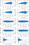 |
Fig. 1 Matching 2MASS and VHS sources. The conversion of the 2MASS to the VHS photometric system is illustrated in the first two rows: the panels in the top row show the magnitude differences for the sample quasars before the correction and the second two rows display the differences after the conversion according to Eq. (1) and Table 1. The deviation at sources brighter than ∼11 mag is related to the saturation in VHS. The astrometric properties are illustrated in the remaining three rows, showing the magnitude differences as a function of the angular separation between VCV10 and 2MASS coordinates, between VCV10 and VHS coordinates, and between the 2MASS and VHS coordinates (top to bottom). Panels on the left are for J, and those on the right are for the K band. |
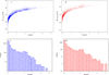 |
Fig. 2 Properties of VCV10 sample. Top: absolute magnitudes in J and K versus redshift, respectively. Bottom: histograms of redshifts of quasars in sample for J and K bands, respectively. They span redshifts up to z ∼ 5.0, but approximately 2/3 have z≤0.5, and only about ∼10% have z>2.0. |
Conversion of VHS magnitudes to 2MASS system.
3.2 Sample curation and variability detection
The filter transmission curves and the detector sensitivity curves of 2MASS and VHS differ, albeit slightly, leading to systematic differences between the magnitudes in the two catalogues. Fig. 1 (top panels) shows this for the VCV10 sample: the deviations are greater for the brighter objects, probably due to non-linearity effects at the image core pixels and because of systematic colour differences between bright and faint objects. To homogenise the data, we introduced a correction, converting the 2MASS magnitudes to VHS magnitudes:
 (1)
(1)
where a and b are the fitting coefficients listed in Table 1. The effect of the correction is shown in Fig. 1 (second top panels). There is an apparent deviation at the bright magnitudes, probably because the pixels in the image cores of the brightest objects saturate. We adopted a cautious approach, omitting objects brighter than 11 mag in any band from our analysis. This condition was applied to the final samples; some plots (e.g. Fig. 1) contain brighter objects to demonstrate the effect of the non-linearity.
Overall, the sample spans a redshift range from 0.003 to 5.1. Fig. 2 shows the absolute magnitude as a function of redshift. The absolute magnitudes were determined assuming H0 = 73.04 km s−1Mpc−1, Ωm = 0.3089, and ΩΛ = 0.6911. We applied K-corrections based on a power-law spectrum with α = 0.5:
 (2)
(2)
Finally, having the corrected magnitudes allows us to identify the AGNs and quasars that show variability at a 3-σ level from
 (3)
(3)
We note that here and throughout the paper the σ is determined based on presumed Poisson photon statistics, which ignores any systematic effects that affect the observations, and, therefore, the quoted significance σ levels must be interpreted with caution. Furthermore, the variability criterion is taken at face value, because with archival surveys there is no control over the time sampling, so any effects such as increasing amplitude with time baseline cannot be accounted for. The sample that meets all these constraints consists of 1571 objects selected based on the J band and 1720 selected based on the K band, or about 22-24% of the quasars with a reliable astrometric match between 2MASS and VHS. 952 objects, or 14%, are variable in both filters above a 3-σ level, and they constitute our final highly variable VCV10-based sample, which is listed in Table 2 and shown in Fig. 3. All these quasars are variable by selection, but the histogram (third panel from top to bottom) and especially the panel with the K versus J band differences (bottom panel) seem to show a valley at above 30-35 σ followed by a group of 16 extremely variable objects in both filters that we paid special attention to. In the subsequent analysis, e.g. for the structure function calculation, we considered the entire sample, so the less variable quasars provided a baseline that helped us determine how the variable quasars can be identified from the comparison of these two surveys, given their accuracy and cadence.
We carried out a search for highly variable objects in Quaia following the same strategy as for the VCV10-based sample; we required a >3σ change between 2MASS and VHS observations in both the J and the K bands to ensure a robust selection. This condition was met by 1493 Quaia quasars, which are listed in Table 3; 167 of these are also present in the VCV10-based sample of variable quasars.
List of 952 variable objects with 2MASS and VHS photometry.
List of 1493 objects selected from the Quaia sample, with photometry from 2MASS and VHS surveys.
3.3 Incompleteness
Our variability sample is based on two quasar samples that suffer from a number of potential problems. These problems are listed below.
The VCV10 sample is extremely heterogeneous, because it was collected from the literature without regard for the selection criteria in the original publications. We can only speculate that the incompleteness is an issue mostly for the faint end, and the bright objects are less affected.
The Quaia quasar sample is based on the original Gaia selection, and for quasars it has a relatively low purity level of 52% (Gaia Collaboration 2023). On the other hand, the spectroscopic confirmation does improve the sample purity, and a comparison with independent redshift measurements shows reasonably good agreement (Ivanov et al. 2024).
The two photometric samples that we used have different completeness limits. Jarrett et al. (2000) reported that our first-epoch 2MASS sample is complete down to J=15.0 mag and KS =13.5 mag. Similar numbers are not available in the main VHS description paper (McMahon et al. 2013), but El Youssoufi et al. (2021, Fig. 5) compared the luminosity functions of 2MASS and different VHS sub-surveys and showed that VHS - which provides our second epoch - is complete to 2.5-3 mag deeper than 2MASS. Of course, this difference depends strongly on the local crowding. It also implies that our selection would miss half of the variable quasars for objects fainter than the 2MASS limits quoted above simply because we would not consider objects that increased their brightness between the two epochs - they would be detected by VSH but missed by 2MASS. To estimate the incompleteness, we counted the quasars in our VCV10-based variable sample that become fainter between the two epochs and those that became brighter. We ignored the completeness limit - which has some uncertainties itself and varies with the stellar density - and included the entire magnitude range. If the two surveys were identical, the two numbers would have been equal. Instead, they differ by 78 in the J band and 66 in the KS bands, which constitutes ∼8% and ∼7% of the 952 objects, respectively. For the Quaia-based sample of variable quasars, the differences in the two bands are 925 and 921, or ∼19% of the 1493 objects. We attribute this to the fact that the VCV10 sample includes more bright, nearby AGNs than the Quaia sample, and, therefore, the incompleteness in the former is expected to be less than in the latter.
Finally, the quasar variability depends on the time lag, and with only two epochs for every object our sample is subject to a bias that is an interplay of the varying time baseline in the observer’s frame and the redshift distribution of the quasars. The available data prevent us from investigating how this affects the completeness of our samples. This question will most likely have to wait for the beginning of the Rubin operations.
Summarising, our samples of variable quasars cannot be considered complete and should not be used for statistical applications that would rely on completeness, e.g., to predict the total number of variable quasars down to a given magnitude limit or redshift.
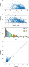 |
Fig. 3 Variability properties of quasars in VCV10 sample. The top panels show the 2MASS versus VHS magnitude change in J and K in units-of-measurement errors added in quadrature from the two surveys. The third panel is the histogram of these deviations for J, K, and the average of the two. The bottom panel plots the normalised deviations in the two bands against each other; the dotted line corresponds to the slope of unity. |
4 Ensemble variability
To investigate the collective variability of the sample, we performed an ensemble analysis of the quasars in common between 2MASS and VHS following the framework of Kouzuma & Yamaoka (2012), which showed it is a powerful tool for studying the physical properties of the nuclear activity, underlying processes, and factors driving their variability. In their framework, the ensemble variability V (i.e., the magnitude change between the two surveys, averaged over all objects in the sample) for a given passband is
 (4)
(4)
where N is the number of objects, Δmi is the magnitude difference, and σi is its observational error  . The uncertainty of V is
 (5)
(5)
In the optical (traditionally limited to λ≤1μm), quasars are known to show weaker variability for a longer rest-frame wavelength (Giallongo et al. 1991; Trèvese & Vagnetti 2002; Vanden Berk et al. 2004; Meusinger et al. 2011). Taking advantage of the wide redshift range covered in our sample, we can verify this relation (with the disclaimer that only 10% of our objects have z>2.0). Our ensemble variability plotted as a function of the rest-frame wavelength is shown in Fig. 4 (top panels) for both J- and K- band data, and we do see a decrease similar to the relations derived by Kouzuma & Yamaoka (2012) and shown in their Fig. 4. The Spearman correlation coefficients are statistically significant: 0.741 for J and 0.806 for K, with 99% significance levels for both filters. The bluest part of the ranges shows an increase, and there are pronounced maxima at around λrest = 0.5-0.6 μm for J and at 0.8 μm for K. One possibility is that these features are due to strong and potentially variable emission lines entering the filters’ band passes and contributing to the measured flux; e.g., Hβ (4861 Å), [OIII] (5007 and 4959 Å), or Hα (6563 Å). However, the sample only includes a few high-z objects, the error bars are larger, and we refrain from drawing firm conclusions.
The relations of the ensemble variability with redshift are also shown in Fig. 4 (middle panels). The quasars are more variable with increasing redshift to z ∼ 1.2 (this limit divides the sample into 80% and 20% fractions) and the variability decreases for more distant objects. The reliability of the observed trends beyond z ∼ 2 is inconclusive due to limited statistics. Finally, the ensemble variability as a function of absolute magnitudes is plotted in the bottom panels. There are peaks at M ∼ −27 mag and −29 mag. For both relations, we observe very similar behaviour to the sample of Kouzuma & Yamaoka (2012, their Figs. 5 and 6).
5 Structure functions
The structure function (SF; Simonetti et al. 1985) is a valuable tool for parametrising the nature of variability for many objects – from irregular variable stars to quasars. It describes the magnitude change between epochs as a function of the time lag between these epochs, and the most useful parameter is the slope of this relation (see Kawaguchi et al. 1998). The sloped part of the SF is bracketed by two flat regions: the lower floor is set by the observational errors while the maximum is defined by the moments of the most extreme variability. The SF has been widely used to study quasars (Hawkins 2002; Vanden Berk et al. 2004; de Vries et al. 2005; Bauer et al. 2009; Schmidt et al. 2010; Kozlowski et al. 2010; Kouzuma & Yamaoka 2012; Kozlowski et al. 2016).
Usually, the SF can be applied to individual objects with multi-epoch monitoring that allows us to probe a range of time lags. Here, we applied it on a large sample of objects with two epochs, because the time intervals between these observations vary from one object to another, so an SF spanning a range of lags can be constructed for the sample as a whole. We caution that the surveys we are using have not been optimised to cover all the regimes of the structure function well, the linear increase sections are not clearly traced, and the large scatter at in some bins makes the choice of the SF fitting range somewhat subjective.
The SFs for the VCV10-based sample are shown in Fig. 5. The points used to fit the SF are marked with larger dots. We considered all quasars and, separately, nearby and distant subsets; these were divided at z=0.5 for the J- band data and at z=1.6 for the K - band data. The limits were selected to facilitate direct comparison with Kouzuma & Yamaoka (2012), and we find similar behaviour to that of the SFs in their Fig. 7; that is, an increase of the variability for rest-frame time lags below ∼1500 d and a decrease for longer lags, giving us confidence in our analysis.
Some of the most relevant theories for explaining the quasar variability are the starburst (Terlevich et al. 1992), instability in the accretion disc (Rees 1984), and microlensing. Kawaguchi et al. (1998) predicted power-law slopes of SF based on various theoretical models. In the starburst (supernova) model, the derived SF slope γ (see Eq. 8 in Kouzuma & Yamaoka 2012) is in the range of ≈0.7-0.9, compared to the SF slope for the accretion-disc instability model, which results in a slope range of ≈0.41-0.49. The model based on microlensing (Hawkins 2002) predicted a slope of ≈0.23-0.31. Hawkins (2002) used the simulated microlensing light curves of Lewis et al. (1993) and Schneider & Weiss (1987) to generate the SF slopes.
We only estimated SF logarithmic slopes γ for the subsets of distant quasars: +0.45 ± 0.18 for J (z>0.5) and +2.28 ± 0.14. for K (z>1.6). The J-band slope overlaps with the ranges reported in Kouzuma & Yamaoka (2012), but the K- band slope appears to be excessively large, probably because of the ill-defined linear section range.
 |
Fig. 4 Ensemble variability V for VCV10 sample as function of rest-frame wavelength (top), redshift (middle, and near-absolute magnitude (bottom) for the J- and K- band data (left and right, respectively). |
6 Discussion
We now look at the collective properties of the quasars and then concentrate on some more prominent individual objects.
6.1 IR ensemble variability and properties of the quasars in other wavelength regimes
There is a discussion of the radio emission, and the quasar optical variability correlation (e.g. Pica & Smith 1983; Bauer et al. 2009). Kouzuma & Yamaoka (2012) reported a weak increase in the IR variability with increasing radio luminosity. To verify this result, we collected 20 cm luminosities for the quasars in the VCV10 sample from Faint Images of the Radio Sky at Twenty Centimeters (FIRST; Becker et al. 1995), and we confirm this trend (Fig. 6, bottom panels). Indeed, the Spearman test yields a positive non-zero coefficient of 0.22 for filter J (p value < 0.001, 95% confidence interval: 0.16 to 0.27) and 0.20 for filter K (p value < 0.001, 95% confidence interval: 0.14 to 0.24). These results suggest a statistically significant (though weak) positive correlation between radio luminosity and IR variability in both the J and K filters.
Next, we compared the IR variability of the objects in the VCV10 sample with the UV and optical ensemble variability estimated by Meusinger et al. (2011) in the r filter from the Sloan Digital Sky Survey (SDSS; York et al. 2000). The results are shown in Fig. 6 (middle panels). Kouzuma & Yamaoka (2012) claimed a weak correlation for the J band and weak anti-correlation for the K band. The Spearman test for our data yields a coefficient of 0.14 for the J band (p value = 0.003, 95% confidence interval: 0.05 to 0.22), indicating a weak but statistically significant positive correlation. For the K band, the coefficient is 0.06 (p value = 0.24, 95% confidence interval: −0.04 to 0.15), suggesting virtually no correlation. Our J- band correlation is slightly stronger than that reported by Kouzuma & Yamaoka (2012), but for K we find negligible evidence of a relationship. A larger data set is needed to draw firmer conclusions, but both our analysis and that of Meusinger et al. (2011) hint - not surprisingly - that quasars may behave more similarly in filters with closer central wavelengths than in filters with more separate wavelengths.
Finally, we compared the magnitude changes of VCV10 quasars with their X-ray luminosities at 0.2-2.3 keV from the Merloni et al. (2024) catalogue, based on observations with the extended ROentgen Survey with an Imaging Telescope Array (eROSITA; Predehl et al. 2020) on board the (SRG; Sunyaev et al. 2021) orbital observatory. For the J band, we find essentially no correlation and with a Spearman coefficient of −0.00008 (p value = 0.998, 95% confidence interval: −0.06 to 0.06). For the K band, we find a very weak positive correlation, with a coefficient of 0.07 (p value = 0.041, 95% confidence interval: −0.004 to 0.12). These results indicate minimal evidence of correlation between X-ray luminosity and IR variability, with only a slight association observed in the K band (Fig. 6 bottom panels).
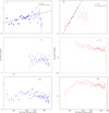 |
Fig. 5 Structure functions for J (left) and K (right) for redshift-selected subsets and for the entire sample. For details, see Sect. 5. |
6.2 Nature of the most variable quasars
We looked at the nature of the most variable objects in the VCV10-based sample, because the original VCV10 sample consists mostly of well-known active galaxies that have been studied for a long time, and they can provide a more definitive picture of the selected objects. We collected their SIMBAD types2, with a clear understanding that this classification is based on heterogeneous data and analysis. Many objects have multiple matches within 2 arcsec with different types, but in most cases, these correspond to detections of the same object at different wavelength regimes; e.g., if an object is a QSO and there are nearby sources in X-ray or UV or radio, we retained the sole QSO type. The distribution of the 852 most variable objects in the VCV10-based sample by type is shown in Fig. 7.
A check of SIMBAD indicates that objects with classifications among both samples of variable objects (based on VCV10 and Quaia - Tables 2 and 3, respectively) are dominated by quasars, Seyferts, BL Lacs, or blazars, but the Quaia sample includes a host of other objects: some of them have been misclassified in the older literature as various types of stars (young stellar objects, various types of variable stars, CVs, etc.), and others are only known by the wavelength range of their detection (IR, radio, etc.). Remarkably, there are 626 objects in the Quaia sample with no classifications (marked as ‘none’ in Fig. 7), and they constitute the single most populated class, underlining the importance of further studies of this new quasar sample. Imposing a requirement for a variability amplitude between the 2MASS and VHS epochs of ten or twenty times the typical observing errors (top and bottom pairs of panels, respectively) removes the majority of objects that were classified in SIMBAD as ‘stellar’ and leaves subsets of objects that have been classified as quasars, BL Lacs, or Seyfert galaxies.
The most variable in the Quaia sample is the well-known z=1.033 flat-spectrum radio quasar (FSRQ) QSO B0208-512. It has already been subjected to rigorous optical spectral monitoring that indicated the redder part of the spectrum is more stable when the object is brighter than the bluer part (Zhang et al. 2022). It is followed by the z=0.506 FSRQ QSO B2232-488 that shows frequently seen redder-when-brighter behaviour in the optical (Zhang et al. 2015) and the z=0.833 blazar [VV2006] J200556.6-231027 (Wallace et al. 2002). The latter object has also been monitored in the optical for variability by Berghea et al. (2021) who find that it showed an amplitude of 1.230 mag in the g band and that the amplitude decreased with wavelength; the smallest amplitude was 0.386 mag in y. This is different from the dominant behaviour in their sample of 2863 quasars that typically exhibit the lowest variability in the r band and the largest in the y band. This contrast hints that our selection did indeed find unusual objects.
To broadly assess how recognised members of our Quaiabased sample of variable quasars are, we searched for them in SIMBAD and found that 587 or ∼39% have no known counterparts within a rather large search radius of 10 arcsec, especially when the average separation for the identified counterparts is 0.6 arcsec. Out of the remaining 908 quasars, 526 have ten or fewer references - they have hardly been studied. One such example is the z=0.08513 Seyfert 1 Galaxy 2MASS J21572316-3123064 - object 43 in Fig. 9, with extremely variable behaviour in the optical (see the next section).
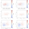 |
Fig. 6 IR variability amplitude in J (left) and K (right) versus X-ray luminosity (top panels), optical variability in the SDSS r band (middle panels), and radio luminosity (bottom panels). The points are coloured by redshift according to the respective colour bars. |
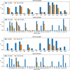 |
Fig. 7 Distributions of SIMBAD object types for VCV10 and Quaia (top and bottom, alternating) samples for different variability levels: the blue histograms show the complete samples and the orange histograms show extremely variable objects with average changes in J and K that exceed 10- and 20-σ significance levels (upper and lower pair of panels). Bracketed numbers in the legends show the number of objects in each set. The bin for objects with no SIMBAD classification is marked with ‘none’. |
6.3 Optical light curves
About 40% of the objects in our selection of extremely variable quasars have been observed with ZTF (we only considered objects with at least 3 observations). The number of epochs usually varies from ∼30 to 890, with an average of 255; the covered time span is between 410 days and 2050 days, with most objects (∼85% for g and ∼90% for r) well above 1800 days (Fig. 8). Some g- band light curves are shown in Fig. 9 with the more variable objects in the near-IR on the top, and, not surprisingly, they tend to show larger variation in the optical as well. However, there are exceptions, such as objects 8 and 16, which show nearly flat light curves.
Our infrared selection is based only on two epochs, so it includes highly variable objects that may have undergone an episodic or short-lived change. We cannot apply a more robust variability indicator for the 2MASS and VHS data sets, but given the significant number of epochs in the ZTF, we can do this for that data set. To exclude outliers and to limit our considerations to objects that do show consistently variable behaviour in the long term - which makes them better suited for e.g., reverberation mapping - we measured the optical amplitude of each light curve as a difference between the 5% and the 95% magnitudes. Furthermore, we normalised this difference by the median observational error for all the observations in that light curve. The histograms of the normalised amplitudes for the 80 most variable objects with available ZTF data and for the 20 least variable in Table 3 are shown in Fig. 10. As expected, the former subset shows systematically larger amplitudes than the latter.
If we tentatively assume that the objects in the first two bins on the left of the histogram are non-variable - an overly pessimistic assumption, because all of them fall well above the 3-σ variability limit by sample construction - then our two-epoch variability criterion allows for ∼11% of non-variable quasar contamination near the least variable end of our ranked sample. This is a strikingly high efficiency level for the selection of variable quasars, given the vast difference in the number of epochs - two for our selection (albeit in two photometric bands) versus the typical number of over two hundred for the ZTF.
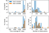 |
Fig. 8 Properties of optical ZTF light curves for the most variable 80 (blue) and for the least variable 20 objects (orange) in our sample. Only optical light curves with at least three observations are included here, which reduces these numbers. Left: histograms of time coverage of light curves for g (top) and r (bottom) filters. Right: same plots for the number of observations. |
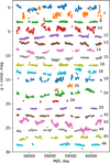 |
Fig. 9 ZTF g- band light curves of subset of most variable Quaia quasars according to the 2MASS-versus-VHS magnitude differences. The number on the right corresponds to the sequential number in Table 3. The observational error bars are smaller than the symbols. |
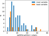 |
Fig. 10 Histograms of 5th and 95th percentile magnitudes for the ZTF light curves of the most and least variable candidates from Table 3. |
7 Summary and conclusions
We selected a sample of nearly 2500 variable quasars for future variability and reverberation studies from the historic VCV10 catalogue and from the recent Quaia quasar catalogue, which identified quasars based on Gaia spectra and mid-infrared colours. Our selection is based on the difference between near-IR J- and K- band observations of 2MASS and VHS, normalised by the observational errors and averaged over the two bands. These two surveys are separated by nearly a decade, which ensures that most of the variable objects exhibit consistently variable behaviour over long timescales.
To verify that 2MASS and VHS surveys cover a representative sample of quasars, we applied an ensemble variability and structure function analysis and compared our results with the work of Kouzuma & Yamaoka (2012), finding good agreement. This strengthened some conclusions about the quasars’ ensemble variability; e.g., that it decreases with the rest-frame wavelength or that it exhibits peaks for certain absolute magnitudes of the quasars. Similarly, the structure function shows an increase in the variability for rest-frame time lags below ∼1500 d and a decrease for longer lags, just like in previous studies. Their trends agree qualitatively with the ones found in optical long-term studies of quasar variability (de Vries et al. 2003, 2005).
Aware of the limited number of observations we used, we investigated if the comparison of only two epochs could provide a reliable selection of variable quasars. Our Quaia-based sample of variable quasars consists of 1493 objects, and ∼40% of them have ZTF optical light curves. We inspected a subset of these, finding that for the strongest candidates our method allows for ∼11% of contamination by quasars that show only weak optical variability. Despite this contamination, we find it remarkably efficient that the comparison of only two epochs in two filters yields results consistent with the analysis of light curves with two orders of magnitude more measurements. A brief inspection of the literature indicated that the vast majority of our Quaia-based variable quasar sample has not been studied in detail before -they are either completely absent from SIMBAD or are only present as entries in various survey catalogues, increasing the value of this sample for further quasar variability studies. A final word of caution: our samples of variable quasars suffer from a number of incompleteness issues and should not be used for statistical studies.
Data availability
Full Tables 2 and 3 are available at the CDS via anonymous ftp to cdsarc.cds.unistra.fr (130.79.128.5) or via https://cdsarc.cds.unistra.fr/viz-bin/cat/J/A+A/699/A52
Acknowledgements
This research has made use of NASA’s Astrophysics Data System Bibliographic Services. This research has made use of the VizieR catalogue access tool, CDS, Strasbourg, France. Topcat (Taylor 2005), Astropy (Astropy Collaboration 2013, 2018) and Matplotlib (Hunter 2007) tools were used in this research. We acknowledge support by Bulgarian National Science Fund under grant DN18-10/2017 and Bulgarian National Roadmap for Research Infrastructure Project D01-326/04.12.2023 of the Ministry of Education and Science of the Republic of Bulgaria.
References
- Amrutha, N., Wolf, C., Onken, C. A., et al. 2024, MNRAS, 535, 2322 [Google Scholar]
- Angione, R. J. 1973, AJ, 78, 353 [Google Scholar]
- Antonucci, R. 1993, ARA&A, 31, 473 [Google Scholar]
- Antonucci, R. 2013, Nature, 495, 165 [Google Scholar]
- Antonucci, R. R. J., & Miller, J. S. 1985, ApJ, 297, 621 [NASA ADS] [CrossRef] [Google Scholar]
- Astropy Collaboration (Robitaille, T. P., et al.) 2013, A&A, 558, A33 [NASA ADS] [CrossRef] [EDP Sciences] [Google Scholar]
- Astropy Collaboration (Price-Whelan, A. M., et al.) 2018, AJ, 156, 123 [Google Scholar]
- Bacon, R., Roth, M. M., Amico, P., & Hernandez, E. 2023, Astron. Nachr., 344, e20230117 [Google Scholar]
- Bauer, A., Baltay, C., Coppi, P., et al. 2009, ApJ, 696, 1241 [NASA ADS] [CrossRef] [Google Scholar]
- Becker, R. H., White, R. L., & Helfand, D. J. 1995, ApJ, 450, 559 [Google Scholar]
- Bellm, E. C., Kulkarni, S. R., Graham, M. J., et al. 2019, PASP, 131, 018002 [Google Scholar]
- Berghea, C. T., Makarov, V. V., Quigley, K., & Goldman, B. 2021, AJ, 162, 21 [Google Scholar]
- Blandford, R. D., & McKee, C. F. 1982, ApJ, 255, 419 [Google Scholar]
- Chen, Y.-C., Liu, X., Liao, W.-T., et al. 2020, MNRAS, 499, 2245 [Google Scholar]
- Cirasuolo, M., Fairley, A., Rees, P., et al. 2020, The Messenger, 180, 10 [NASA ADS] [Google Scholar]
- Dalton, G. B., Caldwell, M., Ward, A. K., et al. 2006, SPIE Conf. Ser., 6269, 62690X [Google Scholar]
- de Jong, R. S., Agertz, O., Berbel, A. A., et al. 2019, The Messenger, 175, 3 [NASA ADS] [Google Scholar]
- de Vries, W. H., Becker, R. H., & White, R. L. 2003, AJ, 126, 1217 [NASA ADS] [CrossRef] [Google Scholar]
- de Vries, W. H., Becker, R. H., White, R. L., & Loomis, C. 2005, AJ, 129, 615 [NASA ADS] [CrossRef] [Google Scholar]
- El Youssoufi, D., Cioni, M.-R. L., Bell, C. P. M., et al. 2021, MNRAS, 505, 2020 [NASA ADS] [CrossRef] [Google Scholar]
- Emerson, J., McPherson, A., & Sutherland, W. 2006, The Messenger, 126, 41 [NASA ADS] [Google Scholar]
- Gaia Collaboration (Bailer-Jones, C. A. L., et al.) 2023, A&A, 674, A41 [NASA ADS] [CrossRef] [EDP Sciences] [Google Scholar]
- Giallongo, E., Trevese, D., & Vagnetti, F. 1991, ApJ, 377, 345 [Google Scholar]
- Greenstein, J. L. 1963, Nature, 197, 1041 [NASA ADS] [CrossRef] [Google Scholar]
- Haardt, F., & Maraschi, L. 1991, ApJ, 380, L51 [Google Scholar]
- Hawkins, M. R. S. 1983, in Liege International Astrophysical Colloquia, 24, Liege International Astrophysical Colloquia, ed. J.-P. Swings, 31 [Google Scholar]
- Hawkins, M. R. S. 2002, MNRAS, 329, 76 [NASA ADS] [CrossRef] [Google Scholar]
- Hawkins, M., & Véron, P. 1990, The Messenger, 61, 46 [Google Scholar]
- Hönig, S. F., & Kishimoto, M. 2011, A&A, 534, A121 [NASA ADS] [CrossRef] [EDP Sciences] [Google Scholar]
- Hook, I. M., McMahon, R. G., Boyle, B. J., & Irwin, M. J. 1994, MNRAS, 268, 305 [Google Scholar]
- Hoyle, F., & Fowler, W. A. 1963a, Nature, 197, 533 [Google Scholar]
- Hoyle, F., & Fowler, W. A. 1963b, MNRAS, 125, 169 [Google Scholar]
- Hunter, J. D. 2007, Comput. Sci. Eng., 9, 90 [NASA ADS] [CrossRef] [Google Scholar]
- Ivanov, V. D., Cioni, M.-R. L., Dennefeld, M., et al. 2024, A&A, 687, A16 [Google Scholar]
- Jarrett, T. H., Chester, T., Cutri, R., et al. 2000, AJ, 119, 2498 [Google Scholar]
- Jiang, Y.-F., & Blaes, O. 2020, ApJ, 900, 25 [NASA ADS] [CrossRef] [Google Scholar]
- Kawaguchi, T., Mineshige, S., Umemura, M., & Turner, E. L. 1998, ApJ, 504, 671 [NASA ADS] [CrossRef] [Google Scholar]
- Kouzuma, S., & Yamaoka, H. 2012, ApJ, 747, 14 [Google Scholar]
- Kozlowski, S., Kochanek, C. S., Stern, D., et al. 2010, ApJ, 716, 530 [CrossRef] [Google Scholar]
- Kozlowski, S., Kochanek, C. S., Ashby, M. L. N., et al. 2016, ApJ, 817, 119 [CrossRef] [Google Scholar]
- Lewis, G. F., Miralda-Escude, J., Richardson, D. C., & Wambsganss, J. 1993, MNRAS, 261, 647 [Google Scholar]
- Lira, P. 2021, in Nuclear Activity in Galaxies Across Cosmic Time, 356, eds. M. Povic, P. Marziani, J. Masegosa, H. Netzer, S. H. Negu, & S. B. Tessema, 101 [Google Scholar]
- López-Navas, E., Sánchez-Sáez, P., Arévalo, P., et al. 2023, MNRAS, 524, 188 [CrossRef] [Google Scholar]
- Maiolino, R., & Rieke, G. H. 1995, ApJ, 454, 95 [Google Scholar]
- Maiolino, R., Alonso-Herrero, A., Anders, S., et al. 2000, ApJ, 531, 219 [NASA ADS] [CrossRef] [Google Scholar]
- Matthews, T. A., & Sandage, A. R. 1963, ApJ, 138, 30 [CrossRef] [Google Scholar]
- McMahon, R. G., Banerji, M., Gonzalez, E., et al. 2013, The Messenger, 154, 35 [NASA ADS] [Google Scholar]
- Merloni, A., Lamer, G., Liu, T., et al. 2024, A&A, 682, A34 [NASA ADS] [CrossRef] [EDP Sciences] [Google Scholar]
- Meusinger, H., Hinze, A., & de Hoon, A. 2011, A&A, 525, A37 [NASA ADS] [CrossRef] [EDP Sciences] [Google Scholar]
- Minev, M., Ivanov, V. D., Trifonov, T., et al. 2021, MNRAS, 508, 2937 [Google Scholar]
- Minev, M., Trifonov, T., Ivanov, V. D., et al. 2024, MNRAS, 531, 4746 [Google Scholar]
- Oke, J. B. 1963, Nature, 197, 1040 [NASA ADS] [CrossRef] [Google Scholar]
- Peterson, B. M. 1993, PASP, 105, 247 [NASA ADS] [CrossRef] [Google Scholar]
- Peterson, B. M., Ferrarese, L., Gilbert, K. M., et al. 2004, ApJ, 613, 682 [Google Scholar]
- Pica, A. J., & Smith, A. G. 1983, ApJ, 272, 11 [NASA ADS] [CrossRef] [Google Scholar]
- Predehl, P., Sunyaev, R. A., Becker, W., et al. 2020, Nature, 588, 227 [CrossRef] [Google Scholar]
- Rees, M. J. 1984, ARA&A, 22, 471 [Google Scholar]
- Rieke, G. H., & Lebofsky, M. J. 1981, ApJ, 250, 87 [NASA ADS] [CrossRef] [Google Scholar]
- Salpeter, E. E. 1964, ApJ, 140, 796 [NASA ADS] [CrossRef] [Google Scholar]
- Sánchez-Sáez, P., Arredondo, J., Bayo, A., et al. 2023, A&A, 675, A195 [NASA ADS] [CrossRef] [EDP Sciences] [Google Scholar]
- Schlafly, E. F., Meisner, A. M., & Green, G. M. 2019, ApJS, 240, 30 [Google Scholar]
- Schmidt, M. 1963, Nature, 197, 1040 [Google Scholar]
- Schmidt, K. B., Marshall, P. J., Rix, H.-W., et al. 2010, ApJ, 714, 1194 [NASA ADS] [CrossRef] [Google Scholar]
- Schneider, P., & Weiss, A. 1987, A&A, 171, 49 [NASA ADS] [Google Scholar]
- Shakura, N. I., & Sunyaev, R. A. 1973, A&A, 24, 337 [NASA ADS] [Google Scholar]
- Shakura, N. I., & Sunyaev, R. A. 1976, MNRAS, 175, 613 [NASA ADS] [CrossRef] [Google Scholar]
- Simonetti, J. H., Cordes, J. M., & Heeschen, D. S. 1985, ApJ, 296, 46 [NASA ADS] [CrossRef] [Google Scholar]
- Sitko, M. L., Sitko, A. K., Siemiginowska, A., & Szczerba, R. 1993, ApJ, 409, 139 [NASA ADS] [CrossRef] [Google Scholar]
- Skrutskie, M. F., Cutri, R. M., Stiening, R., et al. 2006, AJ, 131, 1163 [NASA ADS] [CrossRef] [Google Scholar]
- Smith, H. J., & Hoffleit, D. 1961, PASP, 73, 292 [Google Scholar]
- Smith, H. J., & Hoffleit, D. 1963, Nature, 198, 650 [Google Scholar]
- Storey-Fisher, K., Hogg, D. W., Rix, H.-W., et al. 2024, ApJ, 964, 69 [NASA ADS] [CrossRef] [Google Scholar]
- Sunyaev, R., Arefiev, V., Babyshkin, V., et al. 2021, A&A, 656, A132 [NASA ADS] [CrossRef] [EDP Sciences] [Google Scholar]
- Taylor, M. B. 2005, in Astronomical Society of the Pacific Conference Series, 347, Astronomical Data Analysis Software and Systems XIV, eds. P. Shopbell, M. Britton, & R. Ebert, 29 [Google Scholar]
- Terlevich, R., Tenorio-Tagle, G., Franco, J., & Melnick, J. 1992, MNRAS, 255, 713 [NASA ADS] [CrossRef] [Google Scholar]
- Trèvese, D., & Vagnetti, F. 2002, ApJ, 564, 624 [Google Scholar]
- Trevese, D., Kron, R. G., Majewski, S. R., Bershady, M. A., & Koo, D. C. 1994, ApJ, 433, 494 [NASA ADS] [CrossRef] [Google Scholar]
- Trevese, D., Boutsia, K., Vagnetti, F., Cappellaro, E., & Puccetti, S. 2008, A&A, 488, 73 [NASA ADS] [CrossRef] [EDP Sciences] [Google Scholar]
- Vanden Berk, D. E., Wilhite, B. C., Kron, R. G., et al. 2004, ApJ, 601, 692 [Google Scholar]
- Véron-Cetty, M. P., & Véron, P. 2010, A&A, 518, A10 [Google Scholar]
- Wallace, P. M., Halpern, J. P., Magalhäes, A. M., & Thompson, D. J. 2002, ApJ, 569, 36 [Google Scholar]
- York, D. G., Adelman, J., Anderson, John E. J., et al. 2000, AJ, 120, 1579 [NASA ADS] [CrossRef] [Google Scholar]
- Zhang, B.-K., Zhou, X.-S., Zhao, X.-Y., & Dai, B.-Z. 2015, Res. Astron. Astrophys., 15, 1784 [Google Scholar]
- Zhang, B.-K., Zhao, X.-Y., & Wu, Q. 2022, ApJS, 259, 49 [CrossRef] [Google Scholar]
Information about the SIMBAD types and their hierarchical structure is available at http://vizier.u-strasbg.fr/cgi-bin/OType
All Tables
List of 1493 objects selected from the Quaia sample, with photometry from 2MASS and VHS surveys.
All Figures
|
Fig. 1 Matching 2MASS and VHS sources. The conversion of the 2MASS to the VHS photometric system is illustrated in the first two rows: the panels in the top row show the magnitude differences for the sample quasars before the correction and the second two rows display the differences after the conversion according to Eq. (1) and Table 1. The deviation at sources brighter than ∼11 mag is related to the saturation in VHS. The astrometric properties are illustrated in the remaining three rows, showing the magnitude differences as a function of the angular separation between VCV10 and 2MASS coordinates, between VCV10 and VHS coordinates, and between the 2MASS and VHS coordinates (top to bottom). Panels on the left are for J, and those on the right are for the K band. |
| In the text | |
|
Fig. 2 Properties of VCV10 sample. Top: absolute magnitudes in J and K versus redshift, respectively. Bottom: histograms of redshifts of quasars in sample for J and K bands, respectively. They span redshifts up to z ∼ 5.0, but approximately 2/3 have z≤0.5, and only about ∼10% have z>2.0. |
| In the text | |
|
Fig. 3 Variability properties of quasars in VCV10 sample. The top panels show the 2MASS versus VHS magnitude change in J and K in units-of-measurement errors added in quadrature from the two surveys. The third panel is the histogram of these deviations for J, K, and the average of the two. The bottom panel plots the normalised deviations in the two bands against each other; the dotted line corresponds to the slope of unity. |
| In the text | |
|
Fig. 4 Ensemble variability V for VCV10 sample as function of rest-frame wavelength (top), redshift (middle, and near-absolute magnitude (bottom) for the J- and K- band data (left and right, respectively). |
| In the text | |
|
Fig. 5 Structure functions for J (left) and K (right) for redshift-selected subsets and for the entire sample. For details, see Sect. 5. |
| In the text | |
|
Fig. 6 IR variability amplitude in J (left) and K (right) versus X-ray luminosity (top panels), optical variability in the SDSS r band (middle panels), and radio luminosity (bottom panels). The points are coloured by redshift according to the respective colour bars. |
| In the text | |
|
Fig. 7 Distributions of SIMBAD object types for VCV10 and Quaia (top and bottom, alternating) samples for different variability levels: the blue histograms show the complete samples and the orange histograms show extremely variable objects with average changes in J and K that exceed 10- and 20-σ significance levels (upper and lower pair of panels). Bracketed numbers in the legends show the number of objects in each set. The bin for objects with no SIMBAD classification is marked with ‘none’. |
| In the text | |
|
Fig. 8 Properties of optical ZTF light curves for the most variable 80 (blue) and for the least variable 20 objects (orange) in our sample. Only optical light curves with at least three observations are included here, which reduces these numbers. Left: histograms of time coverage of light curves for g (top) and r (bottom) filters. Right: same plots for the number of observations. |
| In the text | |
|
Fig. 9 ZTF g- band light curves of subset of most variable Quaia quasars according to the 2MASS-versus-VHS magnitude differences. The number on the right corresponds to the sequential number in Table 3. The observational error bars are smaller than the symbols. |
| In the text | |
|
Fig. 10 Histograms of 5th and 95th percentile magnitudes for the ZTF light curves of the most and least variable candidates from Table 3. |
| In the text | |
Current usage metrics show cumulative count of Article Views (full-text article views including HTML views, PDF and ePub downloads, according to the available data) and Abstracts Views on Vision4Press platform.
Data correspond to usage on the plateform after 2015. The current usage metrics is available 48-96 hours after online publication and is updated daily on week days.
Initial download of the metrics may take a while.