| Issue |
A&A
Volume 698, May 2025
|
|
|---|---|---|
| Article Number | A133 | |
| Number of page(s) | 16 | |
| Section | Astrophysical processes | |
| DOI | https://doi.org/10.1051/0004-6361/202554685 | |
| Published online | 06 June 2025 | |
Magnetically driven outflows in the 3D common envelope evolution of massive stars
1
Zentrum für Astronomie der Universität Heidelberg, Astronomisches Rechen-Institut, Mönchhofstr. 12-14, D-69120 Heidelberg, Germany
2
Heidelberger Institut für Theoretische Studien, Schloss-Wolfsbrunnenweg 35, 69118 Heidelberg, Germany
3
Zentrum für Astronomie der Universität Heidelberg, Institut für Theoretische Astrophysik, Philosophenweg 12, 69120 Heidelberg, Germany
4
Max-Planck-Institut für Astrophysik, Karl-Schwarzschild-Str. 1, D-85748 Garching, Germany
5
Max Planck Computing and Data Facility, Gießenbachstraße 2, 85748 Garching, Germany
⋆ Corresponding author: marco.vetter@stud.uni-heidelberg.org
Received:
21
March
2025
Accepted:
17
April
2025
Recent three-dimensional magnetohydrodynamical simulations of the common envelope interaction have revealed the self-consistent formation of bipolar magnetically driven outflows. These outflows are launched from a toroidal structure that has properties of a circumbinary disk. So far, the dynamical impact of bipolar outflows on the common envelope phase remained uncertain, and we aim to quantify its importance in this work. Due to the large computational expense of such simulations, we focus on a specific setup to illustrate the impact on common envelope evolution by comparing two simulations – one with magnetic fields and one without. We used the three-dimensional moving-mesh hydrodynamics code AREPO to perform simulations, focusing on the specific case of a 10 M⊙ red supergiant star with a 5 M⊙ black hole companion. We find that by the end of the magnetohydrodynamic simulations (after ∼1220 orbits of the core binary system), about 6.4% of the envelope mass is ejected through the outflow and contributes to extracting angular momentum from the disk structure and core binary. Given the increased torques induced by the launched material near the core binary, the simulation shows a reduction of the final orbital separation by about 24% compared to the purely hydrodynamical scenario, while the envelope ejection rate exhibits only temporary differences and is dominated by recombination-driven equatorial winds. We further investigated the magnetic field amplification and the launching mechanism of the bipolar outflows. The results are consistent with previous works: The magnetic fields are primarily amplified by strong shear flows and the magnetically driven outflows are launched by a magneto-centrifugal mechanism. The outflows are additionally supported by local shock heating and strong magnetic gradients and originate from a distance of 1.1 times the core binary’s orbital separation from its center of mass. From this and preceding works, we conclude that the magnetically driven outflows and their role in the common envelope phase are a universal aspect of such dynamical interactions and we further discuss possible implementations in analytical and non-magnetic numerical model approaches. We propose an adaptation of the αCE formalism for common envelope interactions, that accounts for magnetic effects, by modifying the final orbital energy with a factor of 1 + Mout/μ, with Mout as the mass ejected through the bipolar outflows and μ as the reduced mass of the core binary.
Key words: magnetohydrodynamics (MHD) / methods: numerical / stars: magnetic field / stars: massive / supergiants / stars: winds / outflows
© The Authors 2025
 Open Access article, published by EDP Sciences, under the terms of the Creative Commons Attribution License (https://creativecommons.org/licenses/by/4.0), which permits unrestricted use, distribution, and reproduction in any medium, provided the original work is properly cited.
This article is published in open access under the Subscribe to Open model. Subscribe to A&A to support open access publication.
1. Introduction
The common envelope (CE) phase is one of the most crucial stages in binary stellar evolution. The result of a CE phase has implications for a wide range of astrophysical phenomena, including gravitational wave emitting compact binaries (e.g., Dominik et al. 2012; Ivanova et al. 2013a; Belczynski et al. 2016; Tauris et al. 2017; Vigna-Gómez et al. 2018; Giacobbo & Mapelli 2018; Moreno et al. 2022; Röpke & De Marco 2023), luminous red novae (Ivanova et al. 2013b; Matsumoto & Metzger 2022; Chen & Ivanova 2024; Hatfull & Ivanova 2025), and planetary nebulae (PNe; e.g., Boffin & Jones 2019; Zou et al. 2020; Ondratschek et al. 2022). While the fraction of PNe emerging from a preceding CE phase remains unknown, a majority of PNe (80–85%, see Sahai & Trauger 1998; Parker et al. 2006) show morphologies characterized by rapid bipolar outflows and a slowly expanding equatorial waist (bipolar PNe; e.g., Imai et al. 2002; Tafoya et al. 2020; Guerrero et al. 2020; Bollen et al. 2020, 2022).
As inferred from recent 3D magnetohydrodynamical (MHD) simulations (Ondratschek et al. 2022; Vetter et al. 2024), strongly bipolar structures can self-consistently form in the CE phase. There, the envelope of a giant star is perturbed by a companion plunging deep into the primary star through gravitational drag (e.g., Paczyński 1976; Ivanova et al. 2013a; Röpke & De Marco 2023 and Schneider et al. 2025). During this in-spiral, the envelope is lifted by the transfer of gravitational energy and angular momentum, leading to either a stable binary formed by the core and the companion (referred to as core binary) or a merging event between the two. Previous 3D simulations of CE evolution have demonstrated that only considering gravitational energy appears to be insufficient to eject the entire envelope (e.g., Ohlmann et al. 2016a; Chamandy et al. 2019; Sand et al. 2020; Lau et al. 2022a,b), and that the transferred angular momentum is aligned with the orbital motion of the system. Hence, the formation of a disk-like transient structure around the central core binary after the plunge-in (if the system is not merging) seems inevitable (Gagnier & Pejcha 2023) before other energy sources (e.g., release of recombination energy leading to toroidal winds) can further erode the former envelope material (Vetter et al. 2024). Simultaneously, the magnetic fields in the envelope are amplified and drive collimated outflows in the polar directions launched from the disk structure, and they leave behind a system with a morphology that is reminiscent of bipolar PNe (Ondratschek et al. 2022). Both disk-like structures and bipolar outflows are formed self-consistently in MHD simulations of different CE models (Moreno et al. 2022; Ondratschek et al. 2022; Vetter et al. 2024).
In this work, we aim to probe this idea through the simulations presented in Vetter et al. (2024). Furthermore, we quantify the impact of the magnetically driven outflows on the outcome of the CE evolution. While it has been hypothesized to be negligible during the dynamic phase of CE evolution (Ondratschek et al. 2022), we showed in the preceding work (Vetter et al. 2024) that the mass transport rates through the bipolar outflows can indeed be as high as 10% of the envelope ejection rate associated with recombination driven winds in the post plunge-in CE system.
To study these aspects, we proceed as follows: In Sect. 2, we summarize our methods and the initial model for this work. We then discuss our results in Sect. 3, where we qualitatively compare the MHD simulation to its purely hydrodynamical counterpart (Sect. 3.1), analyze the magnetic field amplification (Sect. 3.2), investigate the launching mechanisms (Sect. 3.3), and measure the properties of the magnetized outflows with the help of tracer particles (Sect. 3.4). Furthermore, we compare our results to a CE scenario involving a neutron star (NS) companion (with M2 = 1.4 M⊙; Sect. 3.5). Finally, we continue with a discussion in Sect. 4, where we focus on the implications of magnetic fields in the CE events, and we conclude in Sect. 5.
2. Methods
The models analyzed in this work are the same as those presented by Vetter et al. (2024), which are based on Moreno et al. (2022). We briefly summarize key aspects in this work, but we refer to these publications for further details.
The 3D CE simulations presented in this work are conducted with the moving-mesh MHD code AREPO (Springel 2010; Pakmor et al. 2011; Pakmor & Springel 2013). The code employs a second-order finite-volume method for solving the underlying hyperbolic conservation laws. Numerical fluxes are computed at every grid cell boundary with the five-wave Harten–Lax–van Leer–Discontinuities approximate Riemann solver (HLLD, Miyoshi & Kusano 2005). The Powell scheme (Powell et al. 1999; Pakmor & Springel 2013) is used to reduce the strength of magnetic monopoles generated during the simulation. A tree-based algorithm is used to calculate the Newtonian self-gravity (Springel 2010). Additionally, the new refinement approach presented in Vetter et al. (2024) for the cells within the softened potential around the primary core and companion (see Ohlmann et al. 2016b) is applied. To account for recombination energy, we applied the OPAL (Iglesias & Rogers 1996; Rogers et al. 1996; Rogers & Nayfonov 2002) equation of state (EoS) similar to previous CE simulations conducted by, for instance, Sand et al. (2020), Kramer et al. (2020) and Moreno et al. (2022). With these choices, we do not account for radiative cooling effects in our models, and thus our model is that of an “adiabatic” evolution.
The primary star model for our CE setup is a 10 M⊙ red super-giant (RSG) with a radius of 438 R⊙ as described in Moreno et al. (2022). The companion is a 5 M⊙ gravity-only point particle chosen to represent a black hole (BH). A dipolar magnetic seed field is applied to the primary star with a surface field strength1 of 1 μG. Additionally, we insert 799, 212 virtual tracer particles (also referred to as “tracers” in the following) as a Lagrangian component recording the physical properties of the flow. The tracer particles are sampled uniformly across the gas cells such that each represents the same fraction of the total mass of the system. Each tracer particle therefore represents a mass of mtr ≈ 8.32 × 10⁻⁶ M⊙ (see Vetter et al. 2024). Furthermore, we conducted a simulation that has the same setup but without magnetic fields, which we refer to as the “purely hydrodynamical” simulation (also “Hydro” case).
The mass of unbound material is quantified by summing over all cells with positive specific energy, where we distinguish between the following:


Here, ekin, etherm, eint and epot are respectively the specific kinetic, thermal, internal (i.e., the sum of the thermal and the ionization energies) and potential energy2.
3. Results
3.1. MHD versus Hydro
For the MHD and the Hydro model alike, as soon as the companion is placed at the surface of the primary star, it starts plunging deeply into the envelope within the first few orbits (Fig. 1 for t ≲ 500 d). During this inspiralling motion, the density perturbations in the envelope are nearly indistinguishable in the two simulations (cf., Figs. 2a and 2b, and Figs. 2c and 2d) and, consequently, we find a good agreement in the orbital evolution and envelope ejection (Fig. 1). As soon as the systems evolve further, beyond the rapid spiral-in (Fig. 2a, for t ≳ 500 d), we start to observe deviations not only in the orbital separation but also in the unbound mass fractions.
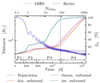 |
Fig. 1. Evolution of the orbital distance and envelope ejection fraction fej for the MHD (thin lines) and Hydro case (thick lines). Shown are the orbital separation (blue) and the fraction of unbound material according to the kinetic, thermal and internal energy criteria, respectively in orange, purple, and green. The black dotted vertical line indicates the starting time of the magnetically driven outflows and the labels “P1” to “P4” represent the different magnetic field amplification phases identified in Sect. 3.2. |
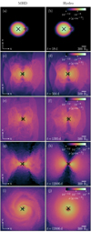 |
Fig. 2. Temporal evolution of the density in the MHD simulation (left) and Hydro simulation (right). Each row shares the same time, orientation, color scale and box size. Panels (a)–(h) are edge-on (x–z) views, while (i) and (j) show the system face-on (x–y). The primary core and companion are marked with a black “x” and “+”, respectively. |
Although the deviations in orbital separation are small after the in-spiral, they become increasingly larger and the orbital separation averaged over the last 20 orbits of the core binary increased from 37 to 46 R⊙ (by ≈24%) in the Hydro case compared to the MHD simulation. Since the core binary can only interact gravitationally with the ambient medium in the simulation, this finding can only be explained by increased gravitational torques in the MHD simulation acting on the binary. Comparing the post spiral-in density structures of the simulations (Fig. 2 and also Movie M1 in Table C.1), it becomes evident that the Hydro case appears less turbulent and more symmetric. Even a clear cavity and evacuated bipolar funnels can be observed in the proximity of the core binary (Fig. 2). The turbulent structures may be traced back to increased stresses by magnetic fields (Gagnier & Pejcha 2024) and in fact, from 200 d on, the magnetic fields become strong enough to extract kinetic energy from the gas (see Appendix A, Fig. A.1). Regardless, a more detailed analysis is required to shed light on the complex mechanism behind the angular momentum transport.
We now study the differences in the evolution of the amount of unbound mass. In both runs, we find recombination-driven winds that dominate the overall envelope ejection process (see also Vetter et al. 2024); they can be most easily identified by the rapid increase in ejected material according to Eq. (1) at t ≈ 1400 d in Fig. 1. In the MHD case, these winds appear about 500 d earlier compared to the Hydro case (see the orange lines in Fig. 1). One might first think of the amplified magnetic fields as a potential explanation for this finding (see Sect. 3.2). But in fact, the total magnetic energy of the entire envelope at about 1400 d is approximately two orders of magnitude below the kinetic energy and furthermore the amplification of the magnetic fields acts as an energy drain, which is the reverse trend of what is needed to explain the earlier onset of the recombination-driven winds. However, there is one energy source that is increasingly contributing to the kinetic energy budget of the system in the MHD case: the larger released orbital energy. In fact, the difference in (averaged) orbital energy between the Hydro and the MHD case at this point is about 2 × 1046 erg and thus approximately comparable to the difference in total kinetic energy between the two simulations (Ekin, MHD − Ekin, Hydro ≈ 1045 erg at 1400 d and up to ≈1046 erg at 2000 d). We thus conclude that the earlier onset of recombination in the MHD case can be traced back to the larger release of orbital energy by the core binary. As the evolution continues, these differences become negligible as the simulations evolve toward full envelope ejection, and the unbound mass fraction follows a similar evolution in both cases for t ≳ 4000 d. However, the most striking difference between the runs is that the MHD model develops high-velocity, collimated, bipolar outflows (see Movie M2 in Table C.1) which carry away angular momentum (Fig. 3), as we show in Sect. 3.4 (see Vetter et al. 2024).
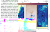 |
Fig. 3. Comparison between the MHD (two plots on the left) and Hydro simulation (two plots on the right) in edge-on slices of radial velocity vr ([a] and [c]) and absolute specific angular momentum |j| ([b] and [d]) with respect to the center of mass of the core binary at t = 4068 d. The MHD simulation shows faster bipolar outflows that carry away a higher specific angular momentum compared to the Hydro case. |
3.2. Magnetic field amplification
As already indicated in Vetter et al. (2024), we observe strong amplification of the seed magnetic fields in our CE simulation, in agreement with Ohlmann et al. (2016a) and Ondratschek et al. (2022). We find an exponential increase in the total magnetic energy by roughly ten orders of magnitude during multiple distinct amplification phases (Fig. 4a).
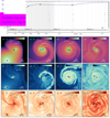 |
Fig. 4. Panel (a): Temporal evolution of the total magnetic energy. The labels “Phase 1” to “Phase 4” are for the different magnetic field amplification phases observed in our simulation (see Sect. 3.2) and the gray shaded region highlights the in-spiral phase defined as the time for which |ȧ/a|P > 0.05, with a being the orbital separation and P being the orbital period. Panels (b)–(e), (f)–(i) and (j)–(m): Density ρ, absolute value of the magnetic field |B| and the absolute value of the local shear rate in the orbital plane |

The first phase takes place during the first orbit up to ∼154 days (see Fig. 4a, the time span labeled as “Phase 1”). It is characterized by the supersonic motion of the companion in the initially only weakly magnetized envelope material within the first orbit (corresponding to the “fast amplification” phase in Ohlmann et al. 2016a). During this phase, the initial perturbation of the envelope creates an accretion stream toward the companion. The spun-up gas in the vicinity of the companion gives rise to locally enhanced shear with respect to the still unperturbed envelope that leads to an amplification of the seed magnetic field (Figs. 4b, 4f and 4j). The expected growth time of the magneto-rotational instability (MRI; Balbus & Hawley 1991) in the fast amplification phase is in our case as short as 2–4 d and approximately matches the e-folding growth time in the magnetic energy of roughly 4 d. In our calculation of the MRI growth rate γMRI and growth time τMRI = γMRI−1, we follow Rembiasz et al. (2016), who give γMRI = qΩ/2, where q is the local rotational shear and Ω is the angular velocity. The first phase is terminated as soon as the companion completed half an orbit and plunged deeply into the envelope of the primary star. At this point in time, the orbital contraction starts to slow (see Fig. 1).
In the second phase (“Phase 2” in Fig. 4a), the spiral-shock arm created within the first orbit (Fig. 4c) expands, becomes unstable, and triggers amplification (Fig. 4g). Along the entire structure, we observe increased shear rates (Fig. 4k), which most likely give rise to Kelvin–Helmholtz instabilities. These phenomena act until ≈380 d and dominate the second amplification phase (the slow amplification phase in Ohlmann et al. 2016b). The expected growth time of the MRI in this phase reaches 90–121 d, which is comparable to the e-folding growth time in Fig. 4a of ∼97 d and thus supports the idea of the MRI being triggered once more as a secular instability superimposed on the shear instability.
Similar to Ondratschek et al. (2022), we observe one additional weak dynamo at play, which is present in the first amplification phase and in the beginning of the second. There, the fluid motion near the primary core leads to an amplified magnetic field strength (Fig. 4f near the core of the primary star).
Although the companion and primary core are still perturbing the remaining envelope and imprinting a spiral pattern in the density profile (e.g., Figs. 4d and 2c), the second amplification phase is terminated after approximately three orbits (≈380 d) and the magnetic energy reaches saturation. In fact, the magnetic energy in the bound material reaches ≈1 − 2% of the total kinetic energy, and we reach equipartition values between the magnetic and turbulent kinetic energy3 of about 30–40%. In this phase, the magnetic energy starts to decrease on timescales on the order of ∼104 d (marked as “Phase 3” in Fig. 4a).
Phase 3 of decreasing magnetic field strength is followed by the third and final amplification phase at around t ∼ 2000 d (labeled “Phase 4” in Fig. 4a). While the requirements are met for the MRI to operate in the bound material (dΩ2/dr < 0; see Vetter et al. 2024), the magnetic energy growth reaches e-folding times of ≈2500 d, which exceed the expected growth time of the linear MRI by an order of magnitude. We also expect linear MRI to be suppressed because the kinetic and magnetic energy densities are comparable at the onset of Phase 4 in the bound material.
Nonetheless, we observe increased shear rates near the core binary (Fig. 4m) which induce further growth in the magnetic energy. The magnetic energy reaches values of about 30–90% of the volume-integrated kinetic energy and even super-equipartion between 1–5 times the turbulent kinetic energy. Hence, the magnetic energy is no longer sourced by turbulent kinetic energy but also by the kinetic energy of the differentially rotating fluid around the core binary. Ondratschek et al. (2022) proposed that this phase may be originating from shear flows induced by mass transfer in the core binary, similar to the case of a main-sequence or WD-NS merger event (Schneider et al. 2019; Morán-Fraile et al. 2024). Further analysis is required to better understand the last magnetic magnetic field amplification phase.
To deepen our understanding of the temporal evolution of the magnetic field amplification, we turned our attention to the evolution equation of the magnetic energy density in an ideal MHD,

where B is the magnetic field, emag = |B|2/2 is the magnetic energy density and v is the velocity. Here, the two terms on the left-hand side of the equation correspond to the temporal change and the transport of magnetic energy in conservation form, while the terms on the right-hand side are associated with stretching and (de-)compression of field lines.
Integrating the individual terms over the entire domain yields the global evolution of the magnetic energy, as shown in Fig. 5. Again, we can identify the four phases indicated previously in Fig. 4. We find that the stretching term dominates the field amplification throughout the entire simulation (similar to the findings in Gagnier & Pejcha 2024). The highest local shear rates (and since  , the fastest amplification; compare with Fig. 4) are found within the spiral arms and near the companion and primary core. Given the strong shock initiated in the perturbed envelope by the plunge-in and the emerging spiral structure afterward, we observe the compression term contributing to the first and partially to the second amplification phase via shock compression of the material. However, during the second half of the second phase (around ≈300 d), the compression term becomes negative due to the expanding envelope material, and the amplification is terminated. Similar to the first two phases, the stretching term increases again in the fourth phase, most likely caused by strong differential rotation near the core binary and close to the spiral pattern as argued before.
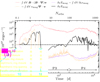 |
Fig. 5. Time evolution of the different terms in the magnetic energy density evolution equation (see Sect. 3.2, Eq. 4) integrated over the entire domain. Shown are the stretching term ∫dV B ⋅ (B ⋅ ∇)v, compression term ∫dV emag∇ ⋅ v, the time derivative of the total magnetic energy ∂t Emag and the numerical dissipation term (∂t Emag − ∫dV ∂t emag) in red, orange, black and violet, respectively. Given the applied periodic boundary condition in our model, the contribution of the advection term vanishes, and for the analysis here we focus on the compression and stretching terms. The time derivative of the magnetic energy ∂tEmag is obtained from the data in Fig. 4a. |
3.3. Magnetic outflow launching
Once the central binary enters the third amplification phase (Phase 4 in Fig. 4a, around 2000 d or 100 orbits; cf., Sect. 3.2), a magnetically driven outflow perpendicular to the orbital plane becomes visible (e.g., Fig. 3). As already stated in Sect. 3.1, we find along the chimney, that is the low density funnel along the z-direction, outflows with enhanced radial velocities carrying away angular momentum and mass (see Figs. 7a and 7b). While in the Hydro case, the outflows exhibit lower velocities and are less persistent over time (even transitioning between unipolar and bipolar; see Movie M2 in Table C.1), the amplified fields in the MHD run boost the acceleration, lead to collimation and create persistent polar outflows. In the Hydro case, the outflows may be understood as local shock heating of material near the core binary pushing gas out of the gravitational potential along the way of least resistance, that is, in the polar direction (Narayan & Yi 1995). This is similar to the findings in Gagnier & Pejcha (2025) and potentially in Lau et al. (2022b). A thermally driven acceleration such as this leads to increased entropy and specific enthalpy in the outflows, which we observed in both of our simulations (Figs. 7m and 7n for the enthalpy and for the entropy we refer to Vetter et al. 2024). However, given the temporal robustness and strength of the bipolar outflow in the MHD case, the acceleration by local shock heating described in Gagnier & Pejcha (2025) can be a contribution, but not the main driving mechanism of the acceleration in our case.
Within the Alfvén surface (the transition between sub- to super-Alfvénic poloidal speeds, marked as a gray contour in the zoomed-in plots on the right-hand side of Fig. 7), the gas is accelerated in the polar direction and the low Alfvén Mach numbers  are accompanied by magnetically dominated flows (β−1 = B2/(8πPgas) > 1, see Figs. 7k and 7l). There, we additionally observe the Maxwell stresses dominating over the centrifugal force BrBϕ/(4πρvϕ2) > 1 (Figs. 7e and 7f) indicating that the magnetic fields govern both the gas’s rotation and the redistribution of angular momentum in the bipolar outflow (García-Segura et al. 2021). Consequently, the magnetic field lines are wound up in the outflows, and we observe the helical structure (Fig. 6) as expected in a magneto-centrifugally driven ejection, such as in the Blandford–Payne mechanism (Blandford & Payne 1982). Furthermore, and in agreement with Ondratschek et al. (2022), we also observe a magnetic field dominated by its poloidal component (Figs. 7g and 7h) near the central binary and low poloidal Alfvén Mach numbers ℳA < 1 in the regions above and below the orbital plane of the central binary (Fig. 7j). Both are again characteristics of the Blandford–Payne mechanism for driving magnetic jets, and this process contributes to the outflow of material in our setup. We further identify regions dominated by the toroidal component of the magnetic field, primarily in the circumbinary material (Fig. 7h) resulting from differential rotation. This effect, even though not as pronounced as in Ondratschek et al. (2022), also contributes to the acceleration, similar to magnetic tower jets (e.g., Uchida & Shibata 1985; Lynden-Bell & Boily 1994).
 |
Fig. 6. Three-dimensional rendering of the magnetic field structure at t = 4950 d. The color represents the absolute magnetic field strength. The core binary is embedded between the two conical structures, and the orbital plane is the x–y plane. |
 |
Fig. 7. Properties of the bipolar outflows at t = 3510 d. Shown are the density ρ in (a) and (b), the absolute value of the magnetic field |B| in (c) and (d), the rϕ-component of the Maxwell stress tensor normalized by the centrifugal force |
The cumulative effect of all mechanisms is to accelerate the gas in the outflowing regions to a maximum radial velocity of vr = 290 km s−1, which is of the same order as the orbital velocity of the central binary ( for t = 2000 − 13 708 d, with Mb and a being the core binary mass and its orbital separation, respectively). The half-opening angle of the funnel varies within ≈8 − 12°, where we determined the opening angle according to the gas cells with velocities exceeding vr = 110 km s−1. Above the Alfvén surface, we observe supersonic (ℳ > 1) and super magneto-sonic speeds (
 , with
  being the Alfvén velocity), progressively increasing with outflowing velocity, that is, the highest radial velocities are observed around the symmetry axis of the outflow, and they decrease with distance to the axis.
3.4. Drifting with the flow: Properties of the bipolar outflow
In the following, we use the implemented tracer particles (see Sect. 2) to analyze the magnetically driven outflow. A tracer particle is considered to be launched by the magnetically driven outflow if, at some point during the simulation, its radial velocity exceeds a critical threshold4, vr, crit. We show results of our analysis assuming different thresholds of vr, crit = 110, 160, 210 km s−1. These choices include the broader outer region of the outflow, the intermediate accelerated areas and the very inner region of the outflowing material, respectively, but exclude material accelerated in the bow shocks, which typically has velocities below 110 km s−1. We note that the smallest considered vr, crit already exceeds the escape velocity from the inner binary at a distance of ≈250 R⊙ (coinciding with the typical distances spanned by the Alfvén-pocket in Fig. 7, gray iso-surfaces) and the typical velocities in the recombination-driven winds of about ∼50 km s−1. For the three criteria, we find a total of 51 077, 30 811 and 12 649 tracer particles to be ejected in the polar directions throughout our simulation.
3.4.1. Origin and trajectory
Given our selected tracer particles in the magnetically driven outflows, we can reconstruct their origin in the stellar structure and trajectory. To obtain the broadest possible overview, we take all tracer particles into account which are found to be launched according to the least constraining condition for the radial velocity (i.e., all tracer particles which exceed vr = 110 km s−1, see Sect. 3.4).
In Fig. 8, we show the initial normalized radial, azimuthal, and polar mass distributions of the entire envelope, and of the mass of the tracer particles launched in the magnetic outflow (normalized by the total envelope mass and total ejected tracer particle mass, respectively). Given that the tracer particles are homogeneously distributed over the entire envelope mass for t = 0 d (Sect. 2), one can directly infer how much the individual mass shells, slices and sections are contributing to the ejection through the magnetically driven outflows. Hence, if the distributions (and their logarithmic derivatives) coincide, each part of the primary star is contributing equally to the bipolar outflow along the corresponding dimension.
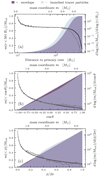 |
Fig. 8. Initial distribution of the launched tracer particles within the envelope. Shown are the normalized cumulative mass distributions m(< x)/Mtot as well as its derivative along the radial (x = r, to 501 R⊙), the polar (x = cos θ) and the azimuthal angle (x = ϕ) in (a), (b) and (c), respectively. The distributions for the total envelope and the launched tracer particle exceeding vr = 110 km s−1 (see Sect. 3.4) are plotted in violet and blue bars, respectively. The derivatives are plotted as black and gray lines. The companion is located at r = 501 R⊙, cosθ = 0 and ϕ = π. |
Analogously, the polar (Fig. 8b) and azimuthal (Fig. 8c) distributions largely overlap; thus, each conical section and slice contributes approximatly equally to the magnetically driven outflows. However, there are small systematic differences. We find a higher contribution from the northern hemisphere as well as the upstream direction of the primary star (around ϕ ≈ π/4) and lower contribution in the downstream region (around ϕ ≈ 3π/4). The difference in the azimuthal direction can be explained due to the immediate interaction of the companion with downstream material within the first half orbit (e.g., see Movie M1 in Table C.1, where this material is first perturbed and partially ejected). The preference toward the northern hemisphere may be traced back to a small asymmetry in the initial position of the companion with respect to the orbital plane, and we encounter this trend once more in Sect. 3.4.3, when we investigate the ejection rates in the outflows.
For the radial direction, however, the outer radial layers of the stellar profile (distances larger than ≈120 R⊙ in Fig. 8a) contribute less to the magnetically launched material as expected for a homogeneous distribution of tracer particles along the envelope. This is due to the outer parts of the envelope being primarily ejected during the plunge-in. However, deeper in the stellar interior, the two distributions overlap, meaning each spherical shell is evenly contributing to the magnetically driven outflow.
This finding is rather surprising, since the companion is spiraling deeper into the initial stellar profile and one would expect an imprint of the CE evolution on the distribution of the launched tracer particles as for the outer parts of the envelope. However, the tracer particles seemingly lose memory of their original positions in the stellar profile provided they survive the plunge-in and form a disk structure. Given that the entire envelope is ejected in our CE scenario (see Sect. 3.1), the tracer particles also serve as a proxy for the post plunge-in envelope. Consequently, the material in the circumbinary disk must also largely lose its dependence on its radial stellar origin. We attribute this finding to the turbulent enhanced transport, as discussed in Vetter et al. (2024).
As for the trajectory of the tracer particles, during the initial rapid spiral-in of the companion (i.e., within the first 750 d), approximately 80% of the envelope material (and all selected tracer particles) are lifted but remain gravitationally bound to the core binary in a torus-like structure (indicated by the blue color in Figs. 9a–9e for t ≲ 2000 d). As the material stays in the orbital plane, the motion of the gas circularizes and is eventually advected toward the central binary (see Vetter et al. 2024 and also Fig. 9), t ≳ 2000 d), until the tracer particles get accelerated and ejected along the polar axis (as indicated by the orange color in Fig. 9). Although this finding of the trajectory of the tracer particles seems trivial, it has previously not been confirmed that the magnetically driven outflow is fueled by a CBD forming from the perturbed but yet gravitationally bound envelope material as proposed in Ondratschek et al. (2022) and Vetter et al. (2024).
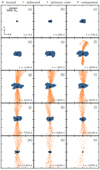 |
Fig. 9. Time evolution of the position of launched tracer particles exceeding a critical velocity of vr = 110 km s−1 (see Sect. 3.4) in the x–z plane. The colors indicate whether the particles are bound (blue) or unbound (orange) according to the kinetic energy criterion in Eq. (1). The primary core and companion positions are marked with a black “+” and “x”, respectively. |
3.4.2. Acceleration region of the magnetically driven outflows
In the following, we try to determine the acceleration region for the magnetically driven outflows (see Sect. 3.3). For our analysis, we focus again on the launched tracer particles based on the least strict radial velocity criterion (i.e., vr = 110 km s−1) to obtain the broadest possible overview (see Sect. 3.4). We perform second-order accurate time derivatives of the velocity of each tracer particle and try to identify a local extrema in the absolute value of the acceleration, where we additionally use the velocity as an identifier to acquire the correct extrema. In this way, we obtain the launching time, which in turn, can be translated to the position of acceleration. One must state, that the data is in general very noisy given the sparse time sampling of 3 d). Consequently, the method does not converge for all tracer particles and about 1842 out of 51 077 are rejected due to difficulties. Nonetheless, we obtain a very broad overview where the particles are preferably accelerated, as we show in the corner plot in Fig. 10. There, the distribution of the acceleration positions along the radial  and absolute vertical direction |z|, centered on the center of mass of the core binary and normalized by the orbital separation at the time of maximum acceleration, is plotted. While the vertical distribution is peaking around the mid-plane (Fig. 10c), the radial distribution shows a pronounced peak around rcyl = 1.1a (i.e., the mode of the distribution).
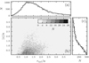 |
Fig. 10. Corner plot of the launching position for all tracer particles exceeding a critical velocity of vr = 110 km s−1 (for the selection process, see Sect. 3.4). In (b), we show the number of tracer particles launched at a given vertical (|z|/a) and cylindrical radial distance (rcyl/a) from the center of mass of the core binary, normalized by the orbital separation at the time of acceleration. In (a) and (c), the marginalized distributions are shown. The mode of the smoothed distribution (piecewise interpolated with a cubic polynomial) in the radial direction is at 1.1a (i.e., the radius with the highest probability for a tracer particle to be launched). |
3.4.3. Measuring outflow rates
In order to measure the properties of the magnetically driven outflow, we count the previously selected tracer particles crossing through a spherical surface with radius r = 5000 R⊙ centered on the center of mass of the core binary within time intervals of Δt = 42 d. This way, we get the time evolution of the mass outflow rate Ṁout, total specific angular momentum |jout| and the angular momentum loss rate |dJout/dt| through the bipolar outflow (Fig. 11). Our findings throughout the different radial velocity criteria are summarized in Table 1 and, in the following, we again illustrate our results for the least strict criterion (i.e., vr, crit = 110 km s−1, see Sect. 3.4) to obtain the broadest possible overview.
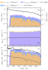 |
Fig. 11. Time evolution of quantities carried away by the launched tracer particles in the polar direction. Shown are the mass-loss rate Ṁout in (a), the specific angular momentum |jout| in (b) and the angular momentum loss rates |dJout/dt| in (c). The colors represent the different critical radial velocities introduced in Sect. 3.4 of vr, crit = 110, 160 and 210 kms−1 in purple, blue and orange, respectively. We additionally show the respective quantities for the CBD in black and for the core binary in dashed gray. With the subscript “out”, we specifically highlight, that the rates shown in this plot are obtained through loss rates of tracer particles passing a control surface within a time window of 42 d (see Sect. 3.4 for more details). |
In total, the tracer particles carry away a mass of Mout, tot = 0.42 M⊙ ≈ 0.064 Menv and the total launched angular momentum amounts to Jout, tot ≈ 9.5 × 1053 g cm2 s−1. The mass-loss rate through the bipolar outflow is approximately an order of magnitude lower than the overall mass ejection rate (Fig. 11a).
We find an average mass-loss rate of ⟨Ṁout⟩t = 3.1 × 10⁻⁵ M⊙ d−1 (see Table 1, with ⟨Q⟩t ≡ ∑jQj/∑j1, the arithmetic mean of quantity Q over all time bins j) which is roughly evenly distributed among both polar directions with a slight preference toward the northern hemisphere (⟨χsym⟩ ≈ 1.2% more mass is ejected through the upper funnel). A similar preference toward the northern hemisphere is already observed in the initial distribution of the tracer particles that are launched in the bipolar outflows (see Sect. 3.4.1) and is caused by slight offset of the companion in the initial condition. Given that the magnetized outflow is refueled by the CBD (Sect. 3.4.1) and in confirmation of the statements in Vetter et al. (2024), these rates recover the reported inward mass fluxes from the CBD material and are roughly a factor of ten smaller than the recombination-driven winds (see Fig. 11a). However, they largely exceed the typical mass-loss rates found in PN observations for jets in post asymptotic giant branch (AGB) binary systems (e.g. Bollen et al. 2020, 2022), or simulations (e.g., García-Segura et al. 2021; Ondratschek et al. 2022) by approximately one to four orders of magnitude. The mass-loss rates are about ∼10−7 − 10−3 × M⊙ yr−1 = 10−9 − 10−6 × M⊙ d−1 in these CE systems with considerably lower-mass AGB primary stars.
Furthermore, we find that the angular momentum loss rates of the magnetically driven outflows almost entirely balance the ones of the CBD, while the loss rates of the core binary remain about one order of magnitude lower. The average angular momentum loss rates are ⟨dJout/dt⟩t ≈ 8.05 × 1044 g cm2 s−2. The specific angular momentum extracted by the outflows (|jout|) remains relatively constant over time (see Fig. 11b) with average values of ⟨jout⟩t ≈ 1.2 × 1021 cm2 s−1. On average, the bipolar outflows extract ⟨jout/jK(r = 1.1a)⟩t = 21.4 times the Keplerian specific angular momentum at the launching point (i.e.,  , see Sects. 3.4.1 and 3.4.2). In fact, this fraction is roughly consistent with the expectations for a Blandford–Payne-like outflow: the fraction of ejected and Keplerian specific angular momentum at the launching point of the disk (jout and jK) is equal to the squared fraction of the distance to the Alfvén surface (RA) and the distance to the launching point (labeled as R here), jout/jK(R) = (RA/R)2. For instance, from Fig. 7, one can infer that RA ≈ 200 R⊙, which yields values ranging from jw/jlaunch = 19 − 35 for an orbital separation of 37 − 50 R⊙.
The number-weighted average velocity of the tracer particles in the outflow is ⟨vr⟩p = 172 km s−1 (here, ⟨Q⟩p ≡ ∑iQi/∑i1, where the summation is taken over each tracer particle i for a given selection method). The time averaged velocity, ⟨vr⟩t = 172 km s−1, shows only minor variations in the evolution, with a standard deviation of ≈14 km s−1. This further supports the conclusion that the magnetically driven acceleration mechanism create continuous outflows. Comparing the radial outflow velocity to the orbital velocity of the core binary, we find typical values of ⟨vr/vorb⟩t = 0.89 averaged over time and 0.91 per tracer particle. Moreover, the average kinetic energy carried away by the outflow (i.e., 0.5Mout⟨vr⟩p2 ≈ 1.3 × 1047 erg) matches the difference in gravitational energy between the Hydro and MHD simulation (i.e.,  ).
).
A comparison between the quantities throughout the regions of the magnetized outflows spanned by the critical velocities can be found in Table 1. For higher critical velocities, the overall picture set forth above remains, but the individual quantities can vary, yet, they remain on the same order of magnitude.
3.5. The neutron star companion
As stated in Vetter et al. (2024), we observe magnetically driven outflows in both CE simulations involving a BH and a NS companion. While most findings in Sect. 3.2 and Sect. 3.3 apply in both cases, we also observe differences between the models. To quantify these differences, we apply the same analysis of the tracer particles to the model involving the NS (see Appendix B, Table B.1). As already stated in Vetter et al. (2024), we observe significant rotation of the orbital plane of the core binary with respect to its initial orientation in the NS scenario, which leads to interactions of the launched and the CBD material. Therefore, unlike in the case of the BH companion, the properties of the jetted outflow may be altered by its interaction with CBD material along its launch direction.
We find similar total specific angular momentum and mass-loss rates in the outflows (also for the core binary and the CBD), although both are subject to larger fluctuations, most likely caused by the pronounced evolution of the orbital plane’s orientation (Vetter et al. 2024). Similar to the q = 0.5 case, the angular momentum loss rate of the core binary is two orders of magnitude below the rates found for the outflows and bound material, while the rates approximately recover the ones in the CBD. The specific angular momentum lost within the time bins is approximately constant and matches the results found in the BH companion scenario of about ⟨|jout|⟩t ≈ 1.16 × 1021 cm2 s−2.
We observe that the post plunge-in orbital contraction rates are in both scenarios similar, which is consistent with our findings in Figs. 11, B.1 and Tables 1, B.1 regarding the angular momentum extraction from the core binary.
We find slightly higher radial velocities for a higher mass ratio. Hence, the outflows reach radial velocities up to 263 km s−1 and on average 164 km s−1, although the orbital velocity of the core binary is found to be higher (at the end of the simulation, vorb = 230 km s−1) compared to the BH companion scenario. Consequently, the average of the fraction of radial velocity and orbital velocity of the core binary is reduced from 0.89 to 0.69.
This finding is opposite to the conclusion in Ondratschek et al. (2022), where the outflow velocities are stronger for less massive companions, given the increased orbital velocity in the tighter orbits of the core binary. It is likely that factors other than the orbital velocity affect the outflow velocity, and wider parameter space exploration could help achieve a complete understanding.
4. Discussion
While this publication focuses on magnetic fields and their impact on the CE evolution, our preceding publications provide extensive discussion on the implications of our initial model and numerical setup on the CE evolution (especially on the orbital separation, eccentricity of the core binary, and envelope ejection), the CBD structure and the final fate of the binary (Moreno et al. 2022; Vetter et al. 2024; Wei et al. 2024). In the following discussion, we focus on the impact of magnetic fields on the CE phase (Sect. 4.2), magnetic field amplification and the launching of the magnetically driven outflows (Sect. 4.1) and lastly, how one can implement our findings in analytical recipes and models that do not explicitly follow the evolution of magnetic fields (Sect. 4.3).
4.1. Magnetic field amplification and launching of bipolar outflows
In Sections 3.2 and 3.3, we analyzed the amplification of magnetic fields and the subsequent launching of material perpendicular to the orbital plane of the central binary. Regarding the first phase of the amplification of magnetic fields, we identified similar mechanisms to those observed in lower-mass systems. However, it is essential to note that other mechanisms might play a significant role, such as, for example, the αΩ-mechanism (e.g., Kiuchi et al. 2024; Pakmor et al. 2024) or other turbulent dynamos. Our analysis is not exhaustive, necessitating more detailed investigations to fully comprehend the amplification processes at play. Special attention must be given to the first amplification phase, because this phase depends sensitively on initial conditions and resolution, which, as argued in Gagnier & Pejcha (2025), leads to underestimated shear rates in numerical simulations. For instance, we neglect any precursory fields existing in the convective envelope of the red supergiant or inherited by the envelope through the preceding phase of binary mass transfer. We also do not account for magnetic fields from the companions themselves (e.g., magnetized white dwarfs, NSs or BHs). Furthermore, we do not resolve the physics nor the scales of actual compact companions on our grid. Moreover, our mass refinement approach is not well-suited to accurately capture magnetic field amplification in low-density regions, leading to underestimated shear rates as argued by Gagnier & Pejcha (2025), although the fastest growing mode of the MRI appears to be resolved in our case. Hence, our results can only be seen as lower limits on the actual growth time in Phase 1 of the magnetic energy. However, as argued by Ohlmann et al. (2016a), the saturation level in Fig. 4 after Phase 2 should be largely independent of the resolution and initial seed field.
Regarding the launching of material, we have identified three mechanisms which contribute to the overall acceleration of material in the polar direction. In agreement with Ondratschek et al. (2022), we find evidence for the Blandford–Payne and the tower jet mechanisms, which are responsible for creating a steady and collimated bipolar outflow with a wound-up magnetic field structure (see Sect. 3.3 and Fig. 6). Indeed, the launching of material is associated with enhanced Maxwell stresses dominating over centrifugal forces and magnetic pressure gradients, which points toward a magneto-centrifugally driven acceleration near the core binary (Sect. 3.3, Fig. 7). In addition (and in agreement with Gagnier & Pejcha 2025), we identified shock-heating of gas close to the central binary to be efficient in accelerating material into the cleared funnel in the polar direction in the Hydro case. This mechanism may also contribute to the overall acceleration in the MHD case, but cannot drive the observed strong outflows in our case. Similar to the arguments presented in Huggins (2012), Blackman & Lucchini (2014), Zou et al. (2020), our results suggest, that the outflows from PNe cannot be explained by the purely hydrodynamical acceleration mechanism.
4.2. Impact of magnetic fields on the CE event
In contrast to Ondratschek et al. (2022), we observe differences in orbital separation and envelope ejection between the strictly hydrodynamical and magnetized models in the CE evolution of our higher-mass system. As stated in Sect. 3.1, the simulation develops bipolar outflows that extract angular momentum from the CBD and the core binary. Consequently, the binary hardens more compared to the purely hydrodynamical simulation. Assuming circular orbits of the core binary and no mass transfer or accretion, the angular momentum of the binary is  , where μ is the reduced mass of the core binary. From that, we can estimate the specific torque difference between the Hydro and the MHD simulation
  , which reaches a minimum of −2.5 × 109 cm2 s−2 at about 3100 d and increases linearly to zero until the end of the simulation. This difference is also reflected in the angular momentum loss rate from the core binary in Fig. 11, given that the core binary in the Hydro run hardly contracts further after 3500 d (see Fig. 1) and the difference is thus dominated by the MHD simulation. The increased stresses on the core binary system may indirectly originate from turbulent enhanced transport rates in the magnetically saturated CBD material by an additional Maxwellian contribution (∝ BrBϕ) (see Vetter et al. 2024). However, to fully understand the angular momentum transport in our simulations, further and more thorough investigations are required, as, for instance, is done in Gagnier & Pejcha (2023, 2024). Furthermore, in the late stages of the evolution (t ≳ 3000 d), we observe changes in eccentricity in the MHD simulation compared to the Hydro scenario (see Fig. 1). As discussed in more detail in Moreno et al. (2022) and Vetter et al. (2024), the eccentricity is numerically not converged in our simulations, but a physical origin can also not be excluded. Future work is warranted to better understand the final eccentricity in our models.
While a more detailed analysis is required to fully unravel the implication of turbulent transport on the CE interactions, we can already draw some conclusions from the results presented in Ondratschek et al. (2022) and this work. The fact, that the outflows appear to form self-consistently in models with different parameters indicates ubiquity of this phenomenon in CE events. However, we expect limits to this universality. For instance, for lower M2, the core and the secondary object can merge or only mildly perturb the envelope5 and neither the magnetic fields can be amplified sufficiently nor the remaining envelope can form a disk-like structure.
In the following discussion, we assume the formation of bipolar outflows and a CBD. The outcome of the CE phase then boils down to the transport of angular momentum and the interaction of the core binary with the disk structure. In the light of enhanced turbulent transport in an effective α-viscous model (Shakura & Sunyaev 1973), one expects α values in the range of 10−2 − 10−1 in the saturated state throughout models (e.g. Davis et al. 2010), but the transport rate will also largely depend on the disk properties such as aspect ratio, local densities and sound speed. While the aspect ratio might arguably be insensitive through different CE scenarios (a thick disk with aspect ratios close to unity seems to form post plunge-in), the local densities and sound speeds in the CBD will depend on the initial primary star and companion model. For the duration of the post plunge-in interaction of the core binary with the CBD (see the systems in, e.g., Vetter et al. 2024), the time increases for increasing M2 and extends even beyond the dynamical interaction as the CE event becomes less adiabatic (e.g., Podsiadlowski 2001). As a result, a long-lived co-existence of the core binary and a disk can be established (e.g., Tuna & Metzger 2023; Wei et al. 2024; Vetter et al. 2024). In light of these thoughts, it is even more surprising that for different companion masses and the given primary model, the relative change in final orbital separation between the models with and without magnetic fields should be comparable, as we argued in Sect. 3.5, and future investigations are required to understand this.
For the envelope ejection process, we do not see significant differences in our simulation between the Hydro and MHD case. The first mass-loss episode can be traced back to the dynamical ejection of about 18–20% of the envelope mass (for t ≲ 1500 d) due to the plunge-in of the companion (see Fig. 1 and also Appendix A, Fig. A.1 for the kinetic energy density evolution), and the MHD and the Hydro simulations coincide. For the subsequent mass ejection event, recombination-driven winds at the edge of the CBD take over and strip the remaining envelope, with mass-loss rates on the order of ∼10−3 − 10−5 M⊙ d−1. These rates exceed those found in the bipolar outflows by about an order of magnitude, and hence, recombination-driven winds largely shape the overall envelope ejection evolution. The recombination-driven winds are likely sensitive to radiative cooling in the remaining envelope material, but this is not included in our adiabatic simulations (see the discussion in Vetter et al. 2024). As argued in (e.g., Meyer & Meyer-Hofmeister 1979; Clayton et al. 2017; Fragos et al. 2019; Bronner et al. 2023) and recently in Lau et al. (2025b), the extended bound envelope can exhibit short radiative transport timescales in the late stages of the interaction and may cause the dominant equatorial envelope ejection to cease.
4.3. Incorporating magnetically driven outflows in other CE models
Based on the results presented here and in Vetter et al. (2024), we develop effective models that allow for the integration of our main results in simplified models of CE evolution. We focus on two aspects: firstly, the formation of bipolar outflows, impacting the orbital separation and envelope ejection already in the dynamical phase of the evolution and, secondly, the implementation of angular momentum transport and extraction from a disk-like structure in the post plunge-in system.
For the first point, we can adjust the αCE energy formalism (van den Heuvel 1976; Webbink 1984) such that we account for the kinetic energy lost through the bipolar outflows in the equation (as argued in Sect. 3.4.3). Since the average ejection velocity per particle is on the order of the orbital velocity of the core binary (see Table 1), we can approximate the kinetic energy carried away by the outflows 0.5Mout⟨vr⟩p2 ≈ 0.5MoutGMb/af with Mout (Sect. 3.4.3), which leads to a modification of the energy formalism:
![$$ \begin{aligned} \alpha _\mathrm{CE} \left[ -\frac{GM_\mathrm{c} M_2}{2a_f}\left(1+\frac{M_\mathrm{out} }{\mu } \right) + \frac{GM_1M_2}{2a_i}\right] = E_\mathrm{bind} , \end{aligned} $$](/articles/aa/full_html/2025/06/aa54685-25/aa54685-25-eq19.gif)
where Ebind is the binding energy of the envelope. This implies that the relative change in final orbital separation for the MHD versus Hydro case is proportional to the fraction of the mass lost in the wind divided by the reduced mass of the core binary af, Hydro/af, MHD = 1 + Mout/μ, which we argued, must be approximately the same for the NS and the BH case due to the insensitivity of the angular momentum loss rates to M2 (Sect. 3.5). In fact, we find Mout/μ to be largely independent of the secondary star mass (for vr, crit = 110, 160, 210 km s−1, we find 0.22, 0.13, 0.06 and 0.19, 0.12, 0.04 for the BH and NS companion, respectively). Furthermore, we can express the mass ejected through the outflow as the time integral over the mass-loss rate  , where we integrate from the onset of the bipolar outflow to the end of the simulation. As stated in Sect. 3.4, the mass-loss rates through the outflows recover the radially inwards mass transport rates in the CBD, which we can express in terms of an effective turbulent α-viscosity (see Vetter et al. 2024). Hence, the ejected mass can be approximated as Mout = 3παθ2Ω∫ΔtΣ(R, t) dt with Ω and θ being the angular velocity and aspect ratio (which are mostly independent of time) and Σ the integrated column density of the CBD at radius R. As one can already infer from this expression, the quantities involved are expected to differ for different primary star models and, for instance, we find Mout/μ ≈ 0.024 for the mass ejection rates reported in Ondratschek et al. (2022) in their q = 0.25 scenario (assuming a linear decay of Ṁ in time and integrating to full envelope ejection from about 1500 d to 4500 d leads to Mout ≈ 0.004 M⊙). As a consistency check, this translates into a final orbital separation of 21.5 R⊙ in their Hydro scenario, coinciding perfectly with the reported final orbital separation of 21.5 R⊙ (taking the reported final orbital separation of 21.0 R⊙ for their MHD simulation). Interestingly, the values for Mout/μ in this work and the ones for Ondratschek et al. (2022) differ by a factor of ten, which is reflected in the quotient of the initial primary star masses.
As for our second point regarding the extraction of angular momentum from the CBD, one can include an effective α-viscosity model to account for the enhanced angular momentum transport found in our MHD case in non-magnetized 1D or multidimensional treatments of the CE interaction. Moreover, an ad hoc central engine with the parameters found in Sect. 3.4 can be employed as used in, for example, Grichener & Soker (2021) and Dori et al. (2023) for 1D models and in, for example, García-Segura et al. (2018, 2020, 2021), and Zou et al. (2020) for multidimensional models.
5. Conclusions
In this work, we have investigated the magnetic field amplification and the launching of magnetized outflows, as well as their implications for the CE evolution of a 10 M⊙ RSG and a 5 M⊙ BH companion. Our results can be summarized as follows:
-
In contrast to the findings in Ondratschek et al. (2022), we observed considerable differences in the orbital separation and envelope ejection between the purely hydrodynamical and magnetized CE evolution. Notably, the final orbital separation of the MHD model is decreased by roughly 24% from 46 R⊙ to 37 R⊙. This difference can be traced back to the enhanced angular momentum transport and the presence of magnetically driven outflows. Consequently, angular momentum is extracted from the core binary by increased torques (as argued in Sect. 4.2). For the envelope ejection, we only observed temporary differences in the ejection process. The deviations are presumably caused by the difference in angular momentum transport; however, the recombination-driven equatorial winds dominate the ejection in our adiabatic setup and the differences disappear by the end of the simulation.
-
We further observed an increase of the magnetic energy by about ten orders of magnitude, and we subdivided the evolution into four distinct phases (see Sect. 3.2). The first phase (rapid amplification phase, Ohlmann et al. 2016b) takes place well within the first orbit and is characterized by strong shear rates during the plunge-in. The second phase (slow amplification phase) is initiated as the spiral arm, which is created within the first orbit, becomes unstable and amplifies the magnetic field in the wake and close to the shock front. The second phase is followed by a decrease of the magnetic field strength (Phase 3) due to magnetic flux conservation and the expanding envelope. In the fourth phase, we again observe strong shear – this time near the central binary – and simultaneously the onset of a bipolar magnetically driven outflow (Sect. 3.3). Our findings are in agreement with earlier works for different CE models (Ohlmann et al. 2016b; Ondratschek et al. 2022). The fact that the evolution is similar in distinct high- and low-mass systems points to a universal amplification mechanism in CE evolution. Firmly establishing this universality, however, requires a wider exploration of the parameter space.
-
While we also observed weak intermittent bipolar ejection in the purely hydrodynamical simulation (similar to Gagnier & Pejcha 2025), the MHD simulation produces strong, stable and collimated ejection of material and angular momentum in the polar direction. In agreement with simulations of low-mass systems (Ondratschek et al. 2022) and even double white dwarf and white dwarf-NS mergers (e.g., Morán-Fraile et al. 2024; Pakmor et al. 2024), we observed indications for both the Blandford–Payne mechanism (Blandford & Payne 1982) and tower-jet-like acceleration. Also in agreement with García-Segura et al. (2021) and their wide-jet prescription, we found increased Maxwell stresses and a steep magnetic pressure gradient in the launching zone. As expected for a magneto-centrifugally launched outflow from a disk, we observed a helical magnetic field structure induced by the circular motion of the gas in the bound material. The material is accelerated up to about vr ≈ 290 km s−1 (on average to 174 km s−1). The structure that arises shares morphological similarities with bipolar PNe (see Ondratschek et al. 2022; Vetter et al. 2024) and magnetized post AGB systems with maser emissions (so called water fountains, e.g., Vlemmings et al. 2006; Khouri et al. 2021, 2025).
-
We further analyzed the outflow with the help of tracer particles (Sect. 3.4). We find that the accelerated material is mostly homogeneously distributed over the initial stellar profile, except for the outer parts of the envelope r ≳ 120 R⊙, which is primarily ejected during the plunge-in. We attribute this finding to efficient mixing in the CBD post plunge-in, which is induced by enhanced turbulent transport (see Sects. 3.4.1, 4.2 and further Vetter et al. 2024). For t ≳ 2000 d, the tracer particles are progressively ejected in the polar directions, where the acceleration area is located around 1.1 times the orbital distance of the core binary and tightly scattered around the orbital plane (see Sect. 3.4.2). Furthermore, we constrained the transport rates of the bipolar outflow (see Sect. 3.4), where we find that ≈6.4% of the envelope mass (nominally 0.42 M⊙) are ejected with an average mass-loss rate of 3.1 × 10⁻⁵ M⊙ d−1. These rates are in agreement with the inward mass transport rates in the CBD (cf., Vetter et al. 2024) and about one order of magnitude below the loss rates produced through recombination-driven winds. The angular momentum extraction by the outflow is consistent with a Blandford–Payne-like outflow (extracting 21.4 times the Keplerian specific angular momentum at the launching point), and on average we found angular momentum loss rates of 8.05 × 1044 g−1 cm2 s−2, which thus balance the rates in the CBD and exceed the ones for the core binary by about one order of magnitude (see Fig. 11 and Table 1 for more details). From the trajectories of the tracer particles (Sect. 3.4.1), we conclude that the outflows are refueled by the remaining bound CBD material.
-
As for the NS companion, the magnetic field amplification as well as the launching mechanisms are identical to those observed in Sects. 3.2 and 3.3, and similar to the findings in Ohlmann et al. (2016a) and Ondratschek et al. (2022). Compared to the q = 0.5 system, the specific angular momentum ejection and mass-loss rates are found to be comparable to the BH companion case, while the total ejected mass is reduced to 0.18 M⊙ (or 2.7% of the envelope). From the similarities between the two simulations, we conclude that the orbital contraction rates induced by the outflows must be comparable in both scenarios.
-
Based on our findings here and in the previous work (Ondratschek et al. 2022; Vetter et al. 2024), we discussed the potential implementation of the effects of a magnetized CE interaction in analytical and numerical approaches. We find that the final orbital energy in the αCE formalism can be adapted by introducing a factor of 1 + Mout/μ and that numerical approaches may include a turbulent α model (Shakura & Sunyaev 1973, for which we reported an effective α of 0.06–0.13 in Vetter et al. 2024) in combination with an ad hoc central engine based on the results reported in Tables 1 and B.1, to mimic the angular momentum loss by the magnetically driven outflows.
In conclusion, we find that the involvement of magnetic fields in the simulation can not only affect the orbital separation but also lead to the self-consistent formation of magnetically driven bipolar outflows, which appears to be a robust outcome of the dynamic interaction. It must be noted that our findings and analysis are far from exhaustive. Future investigations may look into the acceleration area, conduct a more detailed analysis of the field amplification (especially Phase 4), shed light on the mechanisms behind angular momentum transport, refine understanding of the mechanism behind the vertical acceleration in the bipolar outflows (potentially with tracer particles), and study the sensitivity of our findings with regard to the mass ratio and mass of the primary star.
Data availability
Movies associated to Appendix C are available at https://www.aanda.org
For the range in values, we perform volume integrals of the energy densities over a sphere with radius r ∈ [100, 200, 300, 400, 500, 1000] R⊙ centered on the center of mass of the core binary. The equipartition values are computed under the assumption that the turbulent velocity of the gas can be approximated as vturb = (vr, vz)T, where vr, vz are the radial and vertical velocity components in cylindrical coordinates.
For example, in the planetary engulfment scenario (e.g., Lau et al. 2025a), the released orbital energy is orders of magnitude smaller than the binding energy of the star and one may not expect outflows as seen in our simulations.
Acknowledgments
We thank the referee, Dr. Zhuo Chen, for the constructive and helpful review process, which improved the quality of the article. M.V., F.K.R., F.R.N.S., R.A., M.Y.M.L and D.G. acknowledge support by the Klaus-Tschira Foundation. M.Y.M.L. has been supported by a Croucher Foundation Fellowship. M.V., F.K.R., R.A. and D.G. acknowledge funding by the European Union (ERC, ExCEED, project number 101096243). Views and opinions expressed are, however, those of the authors only and do not necessarily reflect those of the European Union or the European Research Council Executive Agency. Neither the European Union nor the granting authority can be held responsible for them. This work has received funding from the European Research Council (ERC) under the European Union’s Horizon 2020 research and innovation program (Grant agreement No. 945806) and is supported by the Deutsche Forschungsgemeinschaft (DFG, German Research Foundation) under Germany’s Excellence Strategy EXC 2181/1-390900948 (the Heidelberg STRUCTURES Excellence Cluster).
References
- Balbus, S. A., & Hawley, J. F. 1991, ApJ, 376, 214 [Google Scholar]
- Belczynski, K., Holz, D. E., Bulik, T., & O’Shaughnessy, R. 2016, Nature, 534, 512 [NASA ADS] [CrossRef] [Google Scholar]
- Blackman, E. G., & Lucchini, S. 2014, MNRAS, 440, L16 [Google Scholar]
- Blandford, R. D., & Payne, D. G. 1982, MNRAS, 199, 883 [CrossRef] [Google Scholar]
- Boffin, H. M. J., & Jones, D. 2019, in The Importance of Binaries in the Formation and Evolution of Planetary Nebulae (Springer Nature Switzerland), SpringerBriefs in Astronomy [Google Scholar]
- Bollen, D., Kamath, D., De Marco, O., Van Winckel, H., & Wardle, M. 2020, A&A, 641, 1 [Google Scholar]
- Bollen, D., Kamath, D., Van Winckel, H., et al. 2022, A&A, 666, A40 [NASA ADS] [CrossRef] [EDP Sciences] [Google Scholar]
- Bronner, V., Schneider, F., Podsiadlowski, P., & Röpke, F. 2023, A&A, 683, A65 [Google Scholar]
- Chamandy, L., Blackman, E. G., Frank, A., et al. 2019, MNRAS, 490, 3727 [NASA ADS] [CrossRef] [Google Scholar]
- Chen, Z., & Ivanova, N. 2024, ApJ, 963, L35 [NASA ADS] [CrossRef] [Google Scholar]
- Clayton, M., Podsiadlowski, P., Ivanova, N., & Justham, S. 2017, MNRAS, 470, 1788 [NASA ADS] [CrossRef] [Google Scholar]
- Davis, S. W., Stone, J. M., & Pessah, M. E. 2010, ApJ, 713, 52 [NASA ADS] [CrossRef] [Google Scholar]
- Dominik, M., Belczynski, K., Fryer, C., et al. 2012, ApJ, 759, 52 [Google Scholar]
- Dori, N., Bear, E., & Soker, N. 2023, ApJ, 954, 143 [Google Scholar]
- Fragos, T., Andrews, J. J., Ramirez-Ruiz, E., et al. 2019, ApJ, 883, L45 [Google Scholar]
- Gagnier, D., & Pejcha, O. 2023, A&A, 674, A121 [NASA ADS] [CrossRef] [EDP Sciences] [Google Scholar]
- Gagnier, D., & Pejcha, O. 2024, A&A, 683, A4 [NASA ADS] [CrossRef] [EDP Sciences] [Google Scholar]
- Gagnier, D., & Pejcha, O. 2025, A\&A, 697, A68 [Google Scholar]
- García-Segura, G., Ricker, P. M., & Taam, R. E. 2018, ApJ, 860, 19 [CrossRef] [Google Scholar]
- García-Segura, G., Taam, R. E., & Ricker, P. M. 2020, ApJ, 893, 150 [CrossRef] [Google Scholar]
- García-Segura, G., Taam, R. E., & Ricker, P. M. 2021, ApJ, 914, 111 [NASA ADS] [CrossRef] [Google Scholar]
- Giacobbo, N., & Mapelli, M. 2018, MNRAS, 480, 2011 [Google Scholar]
- Grichener, A., & Soker, N. 2021, MNRAS, 507, 1651 [Google Scholar]
- Guerrero, M. A., Suzett Rechy-García, J., & Ortiz, R. 2020, ApJ, 890, 50 [NASA ADS] [CrossRef] [Google Scholar]
- Hatfull, R. W. M., & Ivanova, N. 2025, ApJ, 982, 83 [Google Scholar]
- Huggins, P. J. 2012, in Planetary Nebulae: An Eye to the Future, IAU Symposium, 283, 188 [Google Scholar]
- Iglesias, C. A., & Rogers, F. J. 1996, ApJ, 464, 943 [NASA ADS] [CrossRef] [Google Scholar]
- Imai, H., Obara, K., Diamond, P. J., Omodaka, T., & Sasao, T. 2002, Nature, 417, 829 [NASA ADS] [CrossRef] [Google Scholar]
- Ivanova, N., Justham, S., Chen, X., et al. 2013a, A&ARv, 21, 59 [Google Scholar]
- Ivanova, N., Justham, S., Avendano Nandez, J. L., & Lombardi, J. C. 2013b, Science, 339, 433 [NASA ADS] [CrossRef] [Google Scholar]
- Khouri, T., Vlemmings, W. H. T., Tafoya, D., et al. 2021, Nat. Astron., 6, 275 [NASA ADS] [CrossRef] [Google Scholar]
- Khouri, T., Tafoya, D., Vlemmings, W. H. T., et al. 2025, A&A, 694, A222 [NASA ADS] [CrossRef] [EDP Sciences] [Google Scholar]
- Kiuchi, K., Reboul-Salze, A., Shibata, M., & Sekiguchi, Y. 2024, Nat. Astron., 8, 298 [Google Scholar]
- Kramer, M., Schneider, F. R. N., Ohlmann, S. T., et al. 2020, A&A, 642, A97 [NASA ADS] [CrossRef] [EDP Sciences] [Google Scholar]
- Lau, M. Y. M., Hirai, R., González-Bolívar, M., et al. 2022a, MNRAS, 512, 5462 [NASA ADS] [CrossRef] [Google Scholar]
- Lau, M. Y. M., Hirai, R., Price, D. J., & Mandel, I. 2022b, MNRAS, 516, 4669 [NASA ADS] [CrossRef] [Google Scholar]
- Lau, M. Y. M., Cantiello, M., Jermyn, A. S., et al. 2025a, A&A, 694, A264 [NASA ADS] [CrossRef] [EDP Sciences] [Google Scholar]
- Lau, M. Y. M., Hirai, R., Price, D. J., Mandel, I., & Bate, M. R. 2025b, arXiv e-prints [arxiv:2503.20506v1] [Google Scholar]
- Lynden-Bell, D., & Boily, C. M. 1994, MNRAS, 267, 146 [Google Scholar]
- Matsumoto, T., & Metzger, B. D. 2022, ApJ, 938, 5 [NASA ADS] [CrossRef] [Google Scholar]
- Meyer, F., & Meyer-Hofmeister, E. 1979, A&A, 78, 167 [NASA ADS] [Google Scholar]
- Miyoshi, T., & Kusano, K. 2005, J. Comput. Phys., 208, 315 [NASA ADS] [CrossRef] [Google Scholar]
- Morán-Fraile, J., Röpke, F. K., Pakmor, R., et al. 2024, A&A, 681, A41 [NASA ADS] [CrossRef] [EDP Sciences] [Google Scholar]
- Moreno, M. M., Schneider, F. R. N., Röpke, F. K., et al. 2022, A&A, 667, A72 [NASA ADS] [CrossRef] [EDP Sciences] [Google Scholar]
- Narayan, R., & Yi, I. 1995, ApJ, 444, 231 [Google Scholar]
- Ohlmann, S. T., Röpke, F. K., Pakmor, R., Springel, V., & Müller, E. 2016a, MNRAS, 462, L121 [NASA ADS] [CrossRef] [Google Scholar]
- Ohlmann, S. T., Röpke, F. K., Pakmor, R., & Springel, V. 2016b, ApJ, 816, L9 [Google Scholar]
- Ondratschek, P. A., Röpke, F. K., Schneider, F. R. N., et al. 2022, A&A, 660, L8 [NASA ADS] [CrossRef] [EDP Sciences] [Google Scholar]
- Paczyński, B. 1976, in Structure and Evolution of Close Binary Systems, eds. P. Eggleton, S. Mitton, & J. Whelan, IAU Symposium, 73, 75 [NASA ADS] [CrossRef] [Google Scholar]
- Pakmor, R., & Springel, V. 2013, MNRAS, 432, 176 [NASA ADS] [CrossRef] [Google Scholar]
- Pakmor, R., Bauer, A., & Springel, V. 2011, MNRAS, 418, 1392 [NASA ADS] [CrossRef] [Google Scholar]
- Pakmor, R., Pelisoli, I., Justham, S., et al. 2024, A&A, 691, A179 [NASA ADS] [CrossRef] [EDP Sciences] [Google Scholar]
- Parker, Q. A., Acker, A., Frew, D. J., et al. 2006, MNRAS, 373, 79 [NASA ADS] [CrossRef] [Google Scholar]
- Podsiadlowski, P. 2001, in Evolution of Binary and Multiple Star Systems, eds. P. Podsiadlowski, S. Rappaport, A. R. King, F. D’Antona, & L. Burderi, Astronomical Society of the Pacific Conference Series, 229, 239 [NASA ADS] [Google Scholar]
- Powell, K. G., Roe, P. L., Linde, T. J., Gombosi, T. I., & de Zeeuw, D. L. 1999, J. Comput. Phys., 154, 284 [NASA ADS] [CrossRef] [Google Scholar]
- Rembiasz, T., Obergaulinger, M., Cerdá-Durán, P., Müller, E., & Aloy, M. A. 2016, MNRAS, 456, 3782 [NASA ADS] [CrossRef] [Google Scholar]
- Rogers, F. J., & Nayfonov, A. 2002, ApJ, 576, 1064 [Google Scholar]
- Rogers, F. J., Swenson, F. J., & Iglesias, C. A. 1996, ApJ, 456, 902 [Google Scholar]
- Röpke, F. K., & De Marco, O. 2023, Liv. Rev. Comput. Astrophys., 9, 2 [CrossRef] [Google Scholar]
- Sahai, R., & Trauger, J. T. 1998, AJ, 116, 1357 [NASA ADS] [CrossRef] [Google Scholar]
- Sand, C., Ohlmann, S. T., Schneider, F. R. N., Pakmor, R., & Röpke, F. K. 2020, A&A, 644, A60 [NASA ADS] [CrossRef] [EDP Sciences] [Google Scholar]
- Schneider, F. R. N., Ohlmann, S. T., Podsiadlowski, P., et al. 2019, Nature, 574, 211 [Google Scholar]
- Schneider, F. R. N., Lau, M. Y. M., & Roepke, F. K. 2025, arXiv e-prints [arXiv:2502.00111] [Google Scholar]
- Shakura, N. I., & Sunyaev, R. A. 1973, A&A, 24, 337 [NASA ADS] [Google Scholar]
- Springel, V. 2010, MNRAS, 401, 791 [Google Scholar]
- Tafoya, D., Imai, H., Gómez, J. F., et al. 2020, ApJ, 890, L14 [NASA ADS] [CrossRef] [Google Scholar]
- Tauris, T. M., Kramer, M., Freire, P. C. C., et al. 2017, ApJ, 846, 170 [Google Scholar]
- Tuna, S., & Metzger, B. D. 2023, ApJ, 955, 125 [NASA ADS] [CrossRef] [Google Scholar]
- Uchida, Y., & Shibata, K. 1985, PASJ, 37, 515 [NASA ADS] [Google Scholar]
- van den Heuvel, E. P. J. 1976, in Structure and Evolution of Close Binary Systems, eds. P. Eggleton, S. Mitton, & J. Whelan, IAU Symposium, 73, 35 [Google Scholar]
- Vetter, M., Röpke, F. K., Schneider, F. R. N., et al. 2024, A&A, 691, A244 [NASA ADS] [CrossRef] [EDP Sciences] [Google Scholar]
- Vigna-Gómez, A., Neijssel, C. J., Stevenson, S., et al. 2018, MNRAS, 481, 4009 [Google Scholar]
- Vlemmings, W. H. T., Diamond, P. J., & Imai, H. 2006, Nature, 440, 58 [Google Scholar]
- Webbink, R. F. 1984, ApJ, 277, 355 [NASA ADS] [CrossRef] [Google Scholar]
- Wei, D., Schneider, F. R. N., Podsiadlowski, P., et al. 2024, A&A, 688, A87 [NASA ADS] [CrossRef] [EDP Sciences] [Google Scholar]
- Zou, Y., Frank, A., Chen, Z., et al. 2020, MNRAS, 497, 2855 [NASA ADS] [CrossRef] [Google Scholar]
Appendix A: Kinetic energy density evolution
Similarly to the magnetic energy density evolution equation in Eq. (4), one can derive the kinetic energy density evolution equation by multiplying the MHD Euler equation with the velocity and utilizing the continuity equation. The resulting equation reads as
![$$ \begin{aligned} \begin{aligned} \partial _t (\rho e_\mathrm{k} ) + \boldsymbol{\nabla } \cdot (\rho e_\mathrm{k} \boldsymbol{v}) =&- \boldsymbol{\nabla } \cdot (P\boldsymbol{v}) + P \boldsymbol{\nabla } \cdot \boldsymbol{v} + \rho \boldsymbol{g}\cdot \boldsymbol{v} \\&+ \frac{1}{4\pi }[(\boldsymbol{\nabla } \times \boldsymbol{B}) \times \boldsymbol{B}]\cdot \boldsymbol{v}, \end{aligned} \end{aligned} $$](/articles/aa/full_html/2025/06/aa54685-25/aa54685-25-eq21.gif)
with ek = |v|2/2, P, g are the specific kinetic energy, pressure, and gravitational acceleration, respectively. Again, we integrate the evolution equation over the entire domain, which yields the contributions from the different terms in Fig. A.1. From left to right, the two terms on the left-hand side in Eq. (A.1) represent the time derivative of the kinetic energy density and its advection, while the right hand-side accounts for work done by pressure force, (de-) compression (pressure-volume work), gravity and the Lorentz force. The advection and pressure force term can again be ignored, given the periodicity of our domain. As expected, during the first orbit of the companion, orbital energy is directly transferred into the kinetic energy budget of the gas (Fig. A.1), but the main contribution appears to come from pressure-volume work (P∇ ⋅ v), most likely caused by the perturbed hydrostatic equilibrium of the primary star and decompression in the spiral arms. After the first orbit t > 200 d, all terms (except the Lorentz contribution) start to oscillate with the orbital frequency of the binary and dissipation (blue line) is compensating the energy gain by pressure and gravitational work. The magnetic fields start to back react on the fluid flow and contributing as a sink of kinetic energy for the rest of the simulation. As the simulation evolves and the entire envelope is becoming ejected, the change in kinetic energy starts to flatten and converge to zero.
 |
Fig. A.1. Same as Fig. 5 but for the kinetic energy density evolution equation (Eq. A.1). Since we are integrating over the entire domain with periodic boundary conditions, we leave out the advection term and plotted is the derivative of the total kinetic energy of the gas ∂tEk (black), the integrated pressure-volume work term ∫dV P∇ ⋅ v (red), the gravitational term ∫dV ρg ⋅ v (yellow), the Lorentz term ∫dV ([∇ × B]×B)⋅v (violet) and the dissipation term as the residual of the equation ∂tEk − ∫dV∂tρek (blue). |
Appendix B: Measuring the outflow rates in the simulation involving the neutron star companion
Identical to the procedure in Sect. 3.4, we utilize tracer particles to measure the ejection rates through the magnetized outflows in the simulation involving a NS (see Sect. 3.5). The findings are summarized in Table B.1 and Fig. B.1.
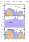 |
Fig. B.1. Same as Fig. 11 but for the simulation involving the NS companion (see Sect. 3.5). For more information, see Sect. . |
Same as Table 1 but for the NS companion (see text in Sect. 3.5).
Appendix C: Movies of the CE interactions
In Table C.1 we summarize the movies presented in this work. There we show the temporal evolution of the density (M1), radial velocity (M2) and absolute magnetic field strength (M3).
Time evolution movies of different quantities for the Hydro and MHD CE simulation.
All Tables
Time evolution movies of different quantities for the Hydro and MHD CE simulation.
All Figures
|
Fig. 1. Evolution of the orbital distance and envelope ejection fraction fej for the MHD (thin lines) and Hydro case (thick lines). Shown are the orbital separation (blue) and the fraction of unbound material according to the kinetic, thermal and internal energy criteria, respectively in orange, purple, and green. The black dotted vertical line indicates the starting time of the magnetically driven outflows and the labels “P1” to “P4” represent the different magnetic field amplification phases identified in Sect. 3.2. |
| In the text | |
|
Fig. 2. Temporal evolution of the density in the MHD simulation (left) and Hydro simulation (right). Each row shares the same time, orientation, color scale and box size. Panels (a)–(h) are edge-on (x–z) views, while (i) and (j) show the system face-on (x–y). The primary core and companion are marked with a black “x” and “+”, respectively. |
| In the text | |
|
Fig. 3. Comparison between the MHD (two plots on the left) and Hydro simulation (two plots on the right) in edge-on slices of radial velocity vr ([a] and [c]) and absolute specific angular momentum |j| ([b] and [d]) with respect to the center of mass of the core binary at t = 4068 d. The MHD simulation shows faster bipolar outflows that carry away a higher specific angular momentum compared to the Hydro case. |
| In the text | |
|
Fig. 4. Panel (a): Temporal evolution of the total magnetic energy. The labels “Phase 1” to “Phase 4” are for the different magnetic field amplification phases observed in our simulation (see Sect. 3.2) and the gray shaded region highlights the in-spiral phase defined as the time for which |ȧ/a|P > 0.05, with a being the orbital separation and P being the orbital period. Panels (b)–(e), (f)–(i) and (j)–(m): Density ρ, absolute value of the magnetic field |B| and the absolute value of the local shear rate in the orbital plane |
| In the text | |
|
Fig. 5. Time evolution of the different terms in the magnetic energy density evolution equation (see Sect. 3.2, Eq. 4) integrated over the entire domain. Shown are the stretching term ∫dV B ⋅ (B ⋅ ∇)v, compression term ∫dV emag∇ ⋅ v, the time derivative of the total magnetic energy ∂t Emag and the numerical dissipation term (∂t Emag − ∫dV ∂t emag) in red, orange, black and violet, respectively. Given the applied periodic boundary condition in our model, the contribution of the advection term vanishes, and for the analysis here we focus on the compression and stretching terms. The time derivative of the magnetic energy ∂tEmag is obtained from the data in Fig. 4a. |
| In the text | |
|
Fig. 6. Three-dimensional rendering of the magnetic field structure at t = 4950 d. The color represents the absolute magnetic field strength. The core binary is embedded between the two conical structures, and the orbital plane is the x–y plane. |
| In the text | |
|
Fig. 7. Properties of the bipolar outflows at t = 3510 d. Shown are the density ρ in (a) and (b), the absolute value of the magnetic field |B| in (c) and (d), the rϕ-component of the Maxwell stress tensor normalized by the centrifugal force |
| In the text | |
|
Fig. 8. Initial distribution of the launched tracer particles within the envelope. Shown are the normalized cumulative mass distributions m(< x)/Mtot as well as its derivative along the radial (x = r, to 501 R⊙), the polar (x = cos θ) and the azimuthal angle (x = ϕ) in (a), (b) and (c), respectively. The distributions for the total envelope and the launched tracer particle exceeding vr = 110 km s−1 (see Sect. 3.4) are plotted in violet and blue bars, respectively. The derivatives are plotted as black and gray lines. The companion is located at r = 501 R⊙, cosθ = 0 and ϕ = π. |
| In the text | |
|
Fig. 9. Time evolution of the position of launched tracer particles exceeding a critical velocity of vr = 110 km s−1 (see Sect. 3.4) in the x–z plane. The colors indicate whether the particles are bound (blue) or unbound (orange) according to the kinetic energy criterion in Eq. (1). The primary core and companion positions are marked with a black “+” and “x”, respectively. |
| In the text | |
|
Fig. 10. Corner plot of the launching position for all tracer particles exceeding a critical velocity of vr = 110 km s−1 (for the selection process, see Sect. 3.4). In (b), we show the number of tracer particles launched at a given vertical (|z|/a) and cylindrical radial distance (rcyl/a) from the center of mass of the core binary, normalized by the orbital separation at the time of acceleration. In (a) and (c), the marginalized distributions are shown. The mode of the smoothed distribution (piecewise interpolated with a cubic polynomial) in the radial direction is at 1.1a (i.e., the radius with the highest probability for a tracer particle to be launched). |
| In the text | |
|
Fig. 11. Time evolution of quantities carried away by the launched tracer particles in the polar direction. Shown are the mass-loss rate Ṁout in (a), the specific angular momentum |jout| in (b) and the angular momentum loss rates |dJout/dt| in (c). The colors represent the different critical radial velocities introduced in Sect. 3.4 of vr, crit = 110, 160 and 210 kms−1 in purple, blue and orange, respectively. We additionally show the respective quantities for the CBD in black and for the core binary in dashed gray. With the subscript “out”, we specifically highlight, that the rates shown in this plot are obtained through loss rates of tracer particles passing a control surface within a time window of 42 d (see Sect. 3.4 for more details). |
| In the text | |
|
Fig. A.1. Same as Fig. 5 but for the kinetic energy density evolution equation (Eq. A.1). Since we are integrating over the entire domain with periodic boundary conditions, we leave out the advection term and plotted is the derivative of the total kinetic energy of the gas ∂tEk (black), the integrated pressure-volume work term ∫dV P∇ ⋅ v (red), the gravitational term ∫dV ρg ⋅ v (yellow), the Lorentz term ∫dV ([∇ × B]×B)⋅v (violet) and the dissipation term as the residual of the equation ∂tEk − ∫dV∂tρek (blue). |
| In the text | |
|
Fig. B.1. Same as Fig. 11 but for the simulation involving the NS companion (see Sect. 3.5). For more information, see Sect. . |
| In the text | |
Current usage metrics show cumulative count of Article Views (full-text article views including HTML views, PDF and ePub downloads, according to the available data) and Abstracts Views on Vision4Press platform.
Data correspond to usage on the plateform after 2015. The current usage metrics is available 48-96 hours after online publication and is updated daily on week days.
Initial download of the metrics may take a while.