© The Authors 2025

1 Introduction

The significant advancements in our observational capabilities during the past decade revealed a large variety of features such as spirals, shadows, gaps, and other non-axisymmetric features in discs that surround forming stars (e.g. Long et al. 2018; Andrews et al. 2018; Cieza et al. 2021, Bae et al. 2023 for a review). Among them, roughly 10% of the observed protoplanetary discs (∼ 30% of the brightest systems) present large 10–100 au dust and gas-depleted cavities that surround their forming stars (see van der Marel 2023 for a review).

Discs with cavities, often referred to as transition discs, belong to the brightest¹ and most frequently studied sources in close star-forming regions (Pinilla et al. 2018; van der Marel et al. 2018; Francis & van der Marel 2020). Their formation has been associated with stellar (e.g. Artymowicz & Lubow 1996; Ragusa et al. 2017; Price et al. 2018) or planetary (e.g. Ataiee et al. 2013; de Juan Ovelar et al. 2013; Regály et al. 2017) companions that interact with the disc. This interaction is a well-known mechanism for depleting the material in the co-orbital region of the companion. Other processes, such as grain growth, dead zones, and photoevaporation, have also been proposed for the formation of these cavities (e.g. Dullemond et al. 2001; Alexander et al. 2006; Regály et al. 2012; Pinilla et al. 2016; Ercolano & Pascucci 2017; van der Marel 2023; Huang et al. 2024).

Although the scenario involving companions appears to be widely invoked in this context, almost no confirmed detections are available in transition disc cavities, with the exception of PDS 70 (Keppler et al. 2018; Müller et al. 2018) and HD 142527, whose binary companion cannot have carved the observed cavity (Nowak et al. 2024). This raises doubts about the companion scenario. Recently, van der Marel et al. (2021) placed observational upper limits on the companion masses in the cavities of several transition discs. The authors concluded that companions with mass ratios q ≳ 0.05 can be excluded in most systems at the location of the gas density minimum. However, it remains possible that companions might be hosted at smaller radii.

Most theoretical works estimated a cavity size a_cav ∼ 2− 4 a_bin, where a_bin is the companion semi-major axis² (e.g. Artymowicz & Lubow 1994; Pichardo et al. 2005; Miranda & Lai 2015; Thun et al. 2017; Zhang et al. 2018; Hirsh et al. 2020; Ragusa et al. 2020; Dittmann & Ryan 2024; Penzlin et al. 2024). Conclusions concerning the detectability of companions based on the observational detection limits mentioned above were typically drawn by comparing the semi-major axis of a putative companion a_bin of a certain mass with the detection limit at location R = a_bin. This is equivalent to assuming an apparent separation of the binary of d = a_bin. However, projection effects that arise because the binary is close to pericentre or to the inclination of the orbit in the plane of the sky can significantly reduce the projected (apparent) separation d of the binary compared to its semi-major axis a_bin. This implies that in a number of instances, a_cav ≫ 4 d and that in order to exclude the presence of companions in a cavity, the comparison with the detection limits also needs to account for the uncertain apparent separation of the putative binary. Figure 1 shows an extreme example from a numerical simulation. It shows an eccentric binary at the pericentre of its highly eccentric orbit (e = 0.8) carving a cavity that features a_cav ∼ 21 d, despite a_cav ∼ 4 a_bin. This causes the binary to appear extremely compact compared to the cavity, and there is a high probability that it remains undetected because the observational resolution in the area is poor (e.g. covered by a coronagraph).

In light of these considerations, we present a novel statistical approach for quantifying the likelihood that a planetary or stellar companion, that is assumed to be carving the cavity, remains undetected because it is located too close to the central star (small projected separation) or too faint to be resolved at the moment of observation. To do this, we produced two samples of companions (one sample for planetary companions, and the other sample for stellar companions) with arbitrarily distributed orbital properties. We studied the resulting projected separations d relative to the binary semi-major axis a_bin(d/a_bin, Sect. 2). Using a disc truncation prescription (Sect. 3), we then studied the size of the cavity a_cav that each companion in the samples would carve in a disc. We calculated the distributions of the projected separations relative to the cavity sizes (d/a_cav, Sect. 4) and their cumulative distributions Sect. (4.1). This quantity acts as the likelihood that a putative companion that carved the cavity remained undetected because the resolution is too low. We then used the observational constraints on the upper mass limits for the companion from van der Marel et al. (2021) to estimate the likelihood that the cavity of a set of real transition discs was carved by undetected stellar or planetary companions because the required sensitivity was lacking (Sect. 4.2). We discuss the results in Sect. 5 and the caveats of our analysis in Sect. 6, and we draw our conclusions in Sect. 7.

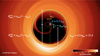Fig. 1 Snapshot of a numerical simulation of a circumbinary disc captured in the extreme situation in which the cavity size acav appears to be larger by a factor ∼21 than the apparent separation d of the binary. The snapshot was produced using the code PHANTOM (Price et al. 2018). It shows a binary with a mass ratio M2/M1 = 0.5, semi-major axis abin = 1, and eccentricity ebin = 0.8 close to its pericentre, that is, with a projected binary separation of d ∼ 0.2 abin. The binary produces a cavity with an eccentricity ecav ∼ 0.2 and a semi-major axis acav ∼ 4.2 abin (consistent with the expected truncation radius by such a binary; see Sect. 3.2), which is equivalent to acav ∼ 21 d. The two white dots mark the position of the two binary stars, and the orange and red ellipses show the orbits of the primary and secondary object, respectively. The binary spends far less time at its pericentre than at the apocentre. It is therefore unlikely that the binary is observed in this configuration, but it is still possible.

2 Samples and projected separations

The projected separation d for a binary with semi-major axis a_bin, inclination i in the plane of the sky, eccentricity e, longitude of pericentre ϖ, and true anomaly f reads (van Albada 1968) $$\frac{d}{a_{\text{bin}}}=\frac{1-e^2}{1+e\cos (f)}{[1-\sin (f+\varpi {)}^2\sin (i{)}^2]}^{1/2}.$$(1)

By assuming the distributions of (f, e, i, ϖ) that are characteristic of a binary population, we can therefore generate the resulting distribution of d/a_bin for the population.

To create the planetary and stellar binary populations, we generated two samples of N = 8.5 × 10⁵ companions with orbital properties (f, e, i, ϖ) specified as follows. The two populations shared the same geometric assumptions for the orientation in space of the orbits: a uniform distribution in 3D space of the orbital inclinations i and the pericentre longitude ϖ, which implies a uniform distribution of cos(i), that is, ${\mathcal{P}}_i=\sin (i)/2$, with i spanning 0 < i < π, and a uniform distribution ${\mathcal{P}}_{\varpi }=1/2\pi$ of the longitude of the pericentres between 0 < ϖ < 2π.

For both populations, the distribution of the true anomalies ${\mathcal{P}}_f$ needs to account for the fact that companions spend more time at the apocentre of their orbit than at the pericentre. This distribution for ${\mathcal{P}}_f$ was obtained by first noting that the binary angular velocity is $\mathrm{d}f/\mathrm{d}t=\mathrm{\Omega }$. As a consequence, the fraction of time dt that a binary spends in one orbit between a true anomaly f and f + df is $$\frac{\mathrm{d}t}{t_{\mathrm{o}\mathrm{r}\mathrm{b}}}=\frac{{\mathrm{\Omega }}_0}{\mathrm{\Omega }}\frac{\mathrm{d}f}{2\pi },$$(2)

where t_orb is the orbital time t_orb = 2π/Ω₀, and Ω₀ = $\sqrt{G{M}_{\text{bin}}/a_{\text{bin}}^3}$, where M_bin is the total mass of the binary. For an eccentric binary, Ω is $$\mathrm{\Omega }={\mathrm{\Omega }}_0\frac{[1+e\cos (f){]}^2}{{[1-e^2]}^{3/2}}.$$(3)

This implies that ${\mathcal{P}}_f$ reads $${\mathcal{P}}_f=\frac{{\mathrm{\Omega }}_0}{2\pi \mathrm{\Omega }}=\frac{{(1-e^2)}^{3/2}}{2\pi [1+e\cos (f){]}^2}.$$(4)

The two populations differ in the distributions we used to generate the eccentricity e and the binary mass ratio q = M₂/M₁, where M₁ and M₂ are the primary and secondary masses of the binary.

For the stellar binary population, we assumed that the distribution ${\mathcal{P}}_{e_{\text{bin}}}$ of the eccentricity e is uniform between 0 ≤ e < 1, while the distribution ${\mathcal{P}}_{q_{\text{bin}}}$ of q is uniform, with q varying between 0.01 ≤ q ≤ 1. This qualitatively reproduces the distributions observed for solar-type field binary stars with separations ranging from few au to ∼ 100 au (Duchêne & Kraus 2013; Moe & Di Stefano 2017; Offner et al. 2023). The choice of the lower limit q = 0.01 for the stellar binary distribution is based on the commonly used 13M_J lower limit for deuterium burning. This sets the threshold mass at which planets are typically considered to be brown dwarfs. For a solar-mass primary star, this limit translates into q ≳ 0.01.

For the planet population, we used the distributions of the eccentricities e, ${\mathcal{P}}_{e_{\mathrm{p}}}$, and the mass ratios q, ${\mathcal{P}}_{q_{\mathrm{p}}}$, from the exoplanet population. We obtained them through a kernel density evaluation (KDE) from the exoplanet dataset (NASA Exoplanet Archive) with a > 2.5 au and q > 5 × 10⁻⁴. The lower limit on the mass ratio here constitutes a conservative estimate of the minimum mass required for gaps to open in the gas and dust density distributions (Dipierro & Laibe 2017; Zhang et al. 2018). The probabilities were obtained by performing the KDE on the log of e and q of the exoplanets and by exploiting the relations ${\mathcal{P}}_e={\mathcal{P}}_{\log e}$/e and ${\mathcal{P}}_q={\mathcal{P}}_{\log q}$/q. A comparison between the exoplanet data and the distributions is shown in Fig. 2. The eccentricity distribution appears to be a Rayleigh distribution, which is consistent with Zhou et al. (2007). We note that we did not correct for observational bias. However, we do not expect observational bias to revert the general properties of ${\mathcal{P}}_{e_{\mathrm{p}}}$ and ${\mathcal{P}}_{q_{\mathrm{p}}}$. A few caveats that derive from our assumptions for the protoplanet population are discussed in Sect. 6.

In Fig. 3, we show the corner plot distributions of (f, e, i, q) of the companions in the two populations. The distribution of ϖ is not plotted because it is uniform. In Fig. 4 we show the resulting ${\mathcal{P}}_{d/a}$ distribution of the quantity d/a_bin for both samples. We note that while e, i, ϖ, and q are not correlated, there is a correlation between e and f, as evident in Fig. 3. This is a consequence of the dependence of ${\mathcal{P}}_f$ on e and f because the higher the binary eccentricity, the longer the time it spends at its apocentre.

The planetary and stellar binary distributions ${\mathcal{P}}_{d/a}$ both peak at a projected separation d/a_bin ∼ 1. However, large tails of projected separations d smaller and larger than a_bin can be noted, with a slightly higher probability for d < a_bin in the planet and stellar binary populations. This effect is stronger in the planetary population: while the eccentricity contributes to producing both d/a_bin ≶ 1, the inclination only reduces the observed projected separation when i ≠ 0. This favours d < a_bin configurations in the planetary population, that is, configurations that are characterised by lower eccentricities. In Appendix A we compare the results obtained with our approach and those obtained by van Albada (1968). The comparison confirms the perfect consistency between the two.

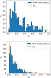Fig. 2 Probability distributions ${\mathcal{P}}_{e_{\mathrm{p}}}$ (top panel) and ${\mathcal{P}}_{q_{\mathrm{p}}}$ (bottom panel) for the eccentricity e and the mass ratio q of the planet population, respectively.

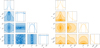Fig. 3 Statistical properties of the samples. Left panel: corner plot distribution of the binary sample we generated for the variables f, e, i, and q for the binary population. Right panel: same as in the left panel, but for the planet population. We deliberately omitted ${\mathcal{P}}_{\varpi }$ because for the binary and planet populations, the longitude of the pericentre ϖ is sampled from a uniform distribution between 0 < ϖ < 2 π. The vertical dashed lines represent intervals containing 16% and 84% of the sample (2σ).

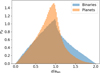Fig. 4 Resulting probability density function (pdf) distributions ${\mathcal{P}}_d$ of the quantity d/abin (Eq. (1)), that is, the ratio of the projected separation of the binary d and its semi-major axis abin, for the stellar binary (shaded blue pdf) and planetary population (shaded orange pdf). The probability density value was obtained by binning the values of d/abin and normalising each bin by ni/Ntot Δ xi, where ni is the number of counts in the bin, Ntot is the total number of elements in the sample, and Δ x is the bin size.

3 Disc truncation

In this section, we introduce a prescription for the disc truncation, based on which we calculated the cavity size a_cav carved by each companion in the samples presented in Sect. 2 if it were surrounded by a protoplanetary disc.

To keep the discussion concise, we briefly introduce the process of disc truncation in Sect. 3.1, and we then introduce in Sect. 3.2 the truncation prescription that is used throughout. Appendix B provides an overview of the literature contextualising our choice for the truncation prescription, and Appendix C contains additional information about the differences and similarities of the two types of truncation mechanisms (resonant and non-resonant).

3.1 General considerations

When a secondary companion mass (a planet or another star) is present in a protoplanetary system, its gravitational potential has two main effects on the surrounding material: (i) It excites waves at resonant locations in the disc (i.e. regions in which the orbital frequency of the companion and the disc have an integer commensurability) that deposit angular momentum and energy in it. This pushes the material (dust/gas) away from the co-orbital region (e.g. Goldreich & Tremaine 1980; Goodman & Rafikov 2001). (ii) It destabilises the orbits of the material and creates regions that are devoid of material (e.g. Rudak & Paczynski 1981; Pichardo et al. 2005). When these mechanisms become sufficiently effective, the gravitational interaction leads to a change in the density structure of the disc.

When the mass ratio q = M₂/M₁ of the companion mass M₂ to the central star M₁ exceeds a certain threshold, a gap opens in the co-orbital region of the companion (for typical protoplanetary disc parameters q > 10⁻³ for a gas-gap opening Crida et al. 2006, and q > 10⁻⁴ for a dust-gap opening Dipierro & Laibe 2017). The typical companions in this gap-forming mass regime are planets that can form characteristic gap features. Inside the gap, the planet is surrounded by a circumplanetary disc or envelope, while a stream of material connects the outer disc with the inner disc across the gap through the L1 and L2 Lagrange points.

For higher mass ratios (q > 0.04), the companion starts to produce a cavity instead of a gap. The structure and dynamics of the disc become more complex and have three distinct components: two circumstellar discs, each of which surrounds the primary and secondary stars and is externally truncated by mutual gravitational interactions; and one circumbinary disc that encompasses both stars and is separated by a material-depleted region known as the cavity. The origin of this transition between the gap and cavity regimes is the lack of horseshoe and/or tadpole-type orbits, that is, stable orbits around the Lagrange points L4 and L5 (Murray & Dermott 1999) for mass ratios q ≳ 0.04.

Despite the substantial dynamical difference between gaps and cavities, numerical simulations of protoplanetary discs have shown that the inner edge of gaps can spread inward (Zhu et al. 2012; Lambrechts et al. 2014; Rosotti et al. 2016; Ubeira Gabellini et al. 2019) when the tidal barrier that is produced by the companion causes dust filtering (i.e. the largest dust grains cannot cross the companion orbit; e.g. Rice et al. 2006) or reduce the gas-accretion rate across the gap, which prevents the inner disc from being refilled with fresh material. This can also produce cavity-like features in the planetary mass regime. Alternatively, a large cavity might be the result of the combined effects of multiple planets such as in the system PDS 70, where two massive planets carve the prominent cavity in the system (Keppler et al. 2018; Bae et al. 2019; Toci et al. 2020a). In these instances, the outermost planet regulates the distance from the cavity edge. In summary, planets and stellar companions produce cavities in discs. This process is also commonly referred to as disc truncation.

The mass and orbital properties of the companions determine the size of the cavity they carve, measured by its semi-major axis a_cav. This is roughly equivalent to the radial extent of the cavity up to moderate values of the cavity eccentricity³ e_cav. Most commonly, a_cav is defined through the gas/dust density as the radial location at which the density Σ becomes a fraction δ = 10−50% of the maximum density value Σ_max at the edge of the cavity, such that Σ(a_cav) = δΣ_max (e.g. Crida et al. 2006; Duffell & Dong 2015; Kanagawa et al. 2018). This is also known as the truncation radius. The value of a_cav can be predicted analytically based on binary-disc interaction theory or numerically with hydrodynamic simulations.

3.2 Truncation prescription in this work

We split our prescription into two separate mass regimes: the stellar companion regime (q > 0.01), and the planetary regime (q < 0.01). The prescriptions provide a smooth transition in the value of a_cav at q = 0.01. We refer to Appendix B for a thorough discussion of truncation mechanisms and their dependence on the system parameters.

For stellar mass companions, we used a truncation prescription based on the 3D stability of the three-body problem by Georgakarakos et al. (2024), which is part of the non-resonant family. The empirical formula of these authors provides the critical semi-major axis of a test particle that orbits a binary with a mass ratio 0.01 ≤ q ≤ 1. Below this critical value, the orbit is found to be unstable for all initial true anomalies. We assumed that this innermost orbit marks the gas-truncation radius. A comparison between this truncation prescription and the results for disc truncation by Pichardo et al. (2005) can be found in Appendix D. The general agreement with the numerical results is good.

The empirical formula from Georgakarakos et al. (2024) expressed as a function of our relevant variables reads $$\begin{array}{rl}{\log }_{10}\left(\frac{a_{\mathrm{c}\mathrm{a}\mathrm{v}}}{a_{\mathrm{b}\mathrm{i}\mathrm{n}}}\right)=& 0.30889-0.26446M_{\mathrm{l}\mathrm{b}}+0.09362i_{\mathrm{d}}\\ & +0.37426e_{\mathrm{b}\mathrm{i}\mathrm{n}}+0.31306e_{\mathrm{c}\mathrm{a}\mathrm{v}}-0.27007M_{\mathrm{l}\mathrm{b}}^2\\ & -0.06102i_{\mathrm{d}}^2-0.09262e_{\mathrm{b}\mathrm{i}\mathrm{n}}^2+0.19436M_{\mathrm{l}\mathrm{b}}{e}_{\mathrm{b}\mathrm{i}\mathrm{n}}\\ & -0.18911i_{\mathrm{d}}{e}_{\mathrm{b}\mathrm{i}\mathrm{n}}-0.05466M_{\mathrm{l}\mathrm{b}}^3+0.06746M_{\mathrm{l}\mathrm{b}}^2{e}_{\mathrm{b}\mathrm{i}\mathrm{n}}\\ & +0.08715i_{\mathrm{d}}^2{e}_{\mathrm{b}\mathrm{i}\mathrm{n}}+1.19488e_{\mathrm{c}\mathrm{a}\mathrm{v}}^3,\end{array}$$(5)

where M_lb = log₁₀(q/q + 1), with q the binary mass ratio, the binary eccentricity e_bin, the test particle inclination (in our case, the mutual binary-disc inclination i_d), and the test particle eccentricity (in our case, the cavity eccentricity e_cav). We refer to Appendix D for an additional discussion of the advantages and motivations for the choice of Eq. (5) as our truncation prescription.

For mass ratios q < 0.01, that is, in the planetary mass regime, we adopted the following prescription: $$\frac{a_{\mathrm{c}\mathrm{a}\mathrm{v}}}{a_{\mathrm{b}\mathrm{i}\mathrm{n}}}=1+e_{\mathrm{b}\mathrm{i}\mathrm{n}}+k\frac{R_{\mathrm{H}\mathrm{i}\mathrm{l}\mathrm{l}}}{a_{\mathrm{b}\mathrm{i}\mathrm{n}}}\sqrt{1-e_{\mathrm{b}\mathrm{i}\mathrm{n}}^2},$$(6)

where R_Hill = a_bin(q/3)^1/3 is the Hill radius, and k = 3.79 is a constant that produces a smooth transition between the planetary and stellar truncation regimes across q = 0.01, as shown in Fig. 5.

This prescription combines multiple features of dependence of the gap width on the planet properties. (i) The known scaling relation of gap widths with the Hill radius Δ = kR_Hill (e.g. Rosotti et al. 2016, as discussed in Appendix B), to which it reduces when e_bin = 0 (a_cav = a_bin + Δ). (ii) The scaling relation found by Chen et al. (2021) that a_cav ∝ 1 + e_bin when a_bin e_bin ≳ R_Hill (i.e. when the planet epicycle exceeds its Hill radius), which agrees qualitatively with orbital stability studies (Petrovich 2015). (iii) The factor $\sqrt{1-e_{\text{bin}}^2}$ enables the smooth connection with the low-mass ratio regime of the Georgakarakos et al. (2024) prescription (Fig. 5). It can be interpreted as a factor that rescales the Hill radius to the average distance R_p between the planet and star along the orbit, a_p $\sqrt{1-e^2}=(2\pi {)}^{-1}{\int }_0^{2\pi }$ R_p df, or as the geometric average between the distance of apocentre and pericentre. (iv) Finally, with proper tuning of k, Eq. (5) produces a smooth transition with the Georgakarakos et al. (2024) prescription at q = 0.01 for all values of e (as shown in Fig. 5). This should be interpreted as an indication that the cavity size indeed depends on q and e_bin also in the q < 0.01 regime: the transition of one curve can be tuned, but the same value of k does not necessarily produce a smooth transition for the other curves as well.

The prescription in Eq. (6) was developed under the assumption that the disc and planet are coplanar, and it does not depend on the mutual disc-planet inclination i_d. This is a reasonable assumption because most exoplanets show low mutual inclinations, which implies that they formed within the disc and continued to orbit close to the disc orbital plane. Similarly to Eq. (5), we assumed that the prescription in Eq. (6) defines the truncation radius of the gaseous disc: by construction, k = 3.79 ensures a smooth transition between the stellar (relevant for the gas) and planetary mass regime. In Sect. 4.2 we discuss an empirical relation that links the size of the gas cavity with that of the dust cavity for a direct comparison with dust continuum sub-millimeter observations.

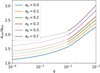Fig. 5 Prescription for acav that combines Eq. (5) for q ≥ 0.01 and (6) for q < 0.01. The transition between the two prescriptions at q = 0.01 is smooth. The different colours represent different values of the planet/binary eccentricity. The dotted lines for q < 0.01 are plotted to highlight the transition between the two prescriptions.

4 Projected separation of the binary for a given cavity size. The distribution of d/a_cav

For each element in the samples that we generated in Sect. 2, we calculated the values of a_cav/a_bin by applying Eq. (5) or (6), depending on their mass ratio. To do this, we assumed the mutual binary/planet-disc inclination i_d, which does not coincide with the inclination in the plane of the sky of the companions i. For the stellar binary case, we prescribed that i_d was a shuffled version of the inclination i array, meaning that binaries and discs have random mutual inclinations (we also tested i_d = 0, i.e. coplanar discs, but there was no significant difference). For the planetary case, as explained in Sect. 3.2, Eq. (6) does not depend on i_d by definition. This implies that the planet and disc are assumed to be coplanar, i_d = 0. As mentioned previously, we considered this to be a reasonable assumption for the planetary case. The top panel of Fig. 6 shows the resulting distribution of a_bin/a_cav, from which we note that stellar companions carve cavities with sizes of a_cav ∼ 2−4 a_bin, and planets carve cavities with sizes of a_cav ∼ 1.5−2 a_bin.

We calculated the ratio of the projected separation d/a_bin obtained in Sect. 2 and a_cav/a_bin to obtain the values of d/a_cav for our samples. Fig. 6 shows the resulting distribution of p(d/a_cav), which provides information about the frequency with which companions with projected separation d carve cavities with a size of a_cav (see Fig. 6).

The planetary and stellar d/a_cav distributions we obtained highlight that cavities are most likely to have projected separations a_cav ∼ 3 d (i.e. d/a_cav ∼ 0.33) for stellar companions and a_cav ∼ 1.7 d (i.e. d/a_cav ∼ 0.7) for planets, which agrees with the respective a_bin/a_cav distributions. However, long tails that extend to d/a_cav ∼ 0 (i.e. a_cav ≫ 3 d) can be observed at smaller projected separations. This highlights the statistical importance of companions at small projected separations.

The physical origin of the difference between the two populations lies in the smaller regions of unstable orbits that surround planets compared to stellar binaries. As a result, the last stable orbits around planets are closer to the co-orbital region than those of stellar binaries. This means that planets carve out smaller cavities than stellar binaries on average, with the same semi-major axis. From another perspective, planets exert a lower tidal torque on the disc than stellar binaries.

In the following sections, we use the statistical information on the projected separations relative to the cavity sizes to study the likelihood that an undetected companion remains undetected within the cavity of transition discs because the spatial resolution is too low (Sect. 4.1), under the assumption that they cause the formation of the cavity. We then extend the analysis by considering limitations of the observational sensitivity (Sect. 4.2).

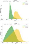Fig. 6 Probability density distribution of abin/acav (top panel) and d/acav (bottom panel). The probability density was obtained by binning the values of d/acav and normalising each bin by ni/Ntot Δ xi, where ni is the number of counts in the bin, Ntot is the total number of elements in the sample, and Δx is the bin size.

4.1 The likelihood that cavity-carving companions remain undetected because the projected separation is small

We started by exploring the case of direct-imaging observations and ignored the possibility that companions might be detected with other techniques, such as radial velocity variations or interferometry (e.g. sparse aperture masking or VLTI-GRAVITY).

A companion that carves the cavity in a transition disc might remain undetected when the projected separation of the binary is too small to be resolved, because the spatial resolution of the instrument is too low, or when it is obscured by a coronagraph during the observations.

We calculated the cumulative distribution of p(d/a_cav) to determine the likelihood of this scenario, $$P(d/a_{\text{cav}}<\mathcal{R})={\int }_0^{\mathcal{R}}p(x)dx.$$(7)

The cumulative probability P(d/a_cav < $\mathcal{R}$) quantifies the percentage of elements in our samples that have d/a_cav < $\mathcal{R}$. This quantity informs us about the fraction of companions in the sample that would not be resolved because they are obstructed by a coronagraph with a size of $\mathcal{R}$ ($\mathcal{R}{a}_{\text{cav}}$ is the coronagraph size in physical units), or more generally, because the resolution over a spatial length $\mathcal{R}$ is too low, and that might be hidden within the cavity.

In Fig. 7, we show these cumulative distributions for the planet and binary samples. We also studied the cumulative distributions after imposing a maximum mass ratio q_max and applying cuts in the binary sample, that is, we removed companions with q > q_max from the sample (see Sect. 4.2 for realistic q_max from real observations). We renormalised the distributions after the cuts to have P(+∞) = 1. This whole procedure is equivalent to changing the initial distribution from which the mass ratios are sampled, and it highlights that different assumptions on the upper limit q_max of the mass ratio affect the likelihood. For a fixed value of $\mathcal{R}$, a lower q_max reduces the probability P for d/a_cav < $\mathcal{R}$. This effect becomes progressively stronger for q_max ≲ 0.1 because a_cav only mildly depends on the binary mass ratio for q > 0.1 (we refer to Appendix B for a discussion of the dependence of a_cav on the system parameters).

We also note that although the shape of the distributions for q and e for generating the planet and stellar companion samples differ strongly, the cumulative distribution for the planet population appears to be a natural extension of the stellar companion with q_max < 0.05, except for some differences in the tails. This suggests that the assumptions on the distribution of e made to generate the samples play a marginal role in determining P(d/a_cav) as long as moderate eccentricities are allowed in the sample, while q_max appears to be the key parameter.

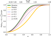Fig. 7 Cumulative distributions P(d/acav < $\mathcal{R}$) calculated using Eq. (7). The solid green and yellow lines show the cumulative distributions for the stellar binary and planetary populations. The dashed lines show distributions obtained by applying a cut q < qmax in the stellar binary regime and renormalising the total distribution to P(d/acav < 1) = 1 to show the impact of q on the cumulative distribution.

4.2 Comparison with the transition disc population

In this section, we extend the previous discussion to include sensitivity detection limits and provide an example of how the statistical approach to disc truncation we presented can be applied to observations. In particular, under the hypothesis that the cavities of transition discs are carved by companions, we calculate the likelihood that they remain undetected, considering the observational detection limits. We note that this is different from the probability that a binary or a planet is present within the cavity, as this analysis does not give us any information about alternative formation mechanisms for cavities. A low likelihood allows us to exclude our hypothesis that a hidden companion carves the cavity, but a high likelihood does not mean that a companion is expected to be found in the cavity.

4.2.1 Sample and definition of the observational truncation radius

We used the sample of transition discs from van der Marel et al. (2021), who collected companion mass detection limits from the literature from sparse aperture masking, coronaph studies, and from lunar occultation. We select 13 systems with cavities from their sample, that is, we excluded systems with dust continuum emission from the central region (no sub-millimeter cavity) and PDS 70, which we know to host two protoplanets that carve its cavity (Bae et al. 2019; Toci et al. 2020a). We did not exclude HD 142527, although its companion with d ∼ 13 au means that it is a circumbinary disc, because recent constraints on its orbit (a_bin ∼ 10 au) appear to suggest that it cannot carve the large cavity of the system (Nowak et al. 2024). This implies that a third unseen body might be present in the system. For such a third body, the constraints from the known binary orbital parameters (q ∼ 0.1, e_bin = 0.47, a_bin = 10.8, i_d = 68^∘, Nowak et al. 2024) suggest that it has a semi-major axis ≳ 30 au in order to have a stable orbit.

We first defined the observational truncation radius $a_{\text{cav}}^{\text{obs}}$ through a direct observable. For this purpose, we chose the radius of the dust ring R_mm (referred to as R_dust by van der Marel et al. 2021), which is defined as the location of the maximum dust emission, and for which a relation of the type $a_{\text{cav}}^{\text{obs}}=ϵR_{\mathrm{m}\mathrm{m}}$ is reasonably expected to obtain the size of the gas cavity – this is required so that we can apply our truncation prescription.

We found that ϵ = 0.75 produces a value of $a_{\text{cav}}^{\text{obs}}$(R_mm) that compares well with the theoretical value a_cav from Eqs. (5) and (6) using as input parameters the real orbital parameters of companions in the four systems in which the orbits of companion were constrained: PDS 70 (Wang et al. 2021), V892 Tau (Long et al. 2021), IRAS 04158 + 2805 (Ragusa et al. 2021), and GG Tau (Keppler et al. 2020; Toci et al. 2024) (see Table 1 for the details of the comparison).

To support our empirical choice of the relation $a_{\text{cav}}^{\text{obs}}(R_{\text{mm}})$ and for the fine-tuning of ϵ = 0.75, we also note the following:

• (i)

  Assuming that the dust ring traces the gas pressure maximum, the characteristic radius used to define the edge of the cavity is usually the location at which the density reaches a fraction of its maximum value (0.1−0.5 × Σ_max; e.g. Crida et al. 2006). The characteristic length scale for the density gradient of a stable gap cannot be shorter than the disc vertical scale height, which implies that the edge of the gas cavity must be at a distance of at least ≳ H from the dust density peak. By definition, this constrains 1−ϵ > H/R.

• (ii)

  The scaling of $a_{\text{cav}}^{\text{obs}}\left(R_{\text{mm}}\right)$ agrees qualitatively with the relation between radius of the gas component and R_CO and R_mm discussed in Facchini et al. (2018), where R_CO/R_mm = ϵ ∼ 0.6–0.85.

• (iii)

  Using ϵ > 0.75, that is, making the prescription more constrained, implies larger $a_{\text{cav}}^{\text{obs}}$ gas cavities. For these to be carved, companions with larger a_bin are required. This would make companions more easily detectable and would lower the likelihood that a companion remains undetected. As a consequence, the likelihood of hidden companions in a system that is already unlikely to host them does not increase simply because ϵ has been adjusted to a higher value. As a result, our choice of ϵ is conservative.

4.2.2 Companion mass detection limits and likelihood

The companion mass detection limits collected by van der Marel et al. (2021) are still currently valid, to our knowledge. The authors collected detection limits in the literature that were mainly obtained based on two methods⁴: (i) coronagraph studies, which provided upper detection limits q_cor on the companion mass ratio outside the coronagraph area at radii R_cor ∼ 0.1−0.2 arcsec; (ii) when available, sparse aperture masking, which provides an upper detection limit q_sp on the companion mass ratio at radii of typically R_sp ≲ 0.2 arcsec. Therefore, we introduced q_max(R) detection limits as continuous functions of the distance from the centre of the system R. This combines the upper limits that were obtained with different methods in each system.

We defined q_max(R) based on a visual estimation from the continuous functions reported in Fig. 4 of van der Marel et al. (2021). For each detection curve in van der Marel et al. (2021), we defined two piecewise detection curves: one $q_{\text{max}}^{+}$ constitutes an optimistic detection limit, and the other $q_{\text{max}}^{-}$ constitutes a conservative detection limit. The optimistic $q_{\text{max}}^{+}$ reads $$q_{max}^{+}(R)=min\left\{\begin{array}{cc}{q}_{\mathrm{s}\mathrm{p}}^{+},& 0\le R\le R_{\mathrm{s}\mathrm{p}}\\ q_{\mathrm{c}\mathrm{o}\mathrm{r}}^{+},& R_{\mathrm{c}\mathrm{o}\mathrm{r}}\le R\le a_{\mathrm{c}\mathrm{a}\mathrm{v}}^{\text{obs\hspace{0.17em}}}\end{array}\right\},$$(8)

where $q_{\mathrm{s}\mathrm{p}}^{+}$ and $q_{\mathrm{c}\mathrm{o}\mathrm{r}}^{+}$ are the maximum values of the detection curves in the sparse masking (0 ≤ R ≤ R_sp) and coronagraph regions (R_cor ≤ x ≤ R_cav), respectively; R_sp is the outer radius of the sparse masking, and R_cor is the coronagraph radius. The min (…) function is required because in some cases R_sp > R_cor.

The conservative $q_{\text{max}}^{-}$ reads $$q_{\mathrm{m}\mathrm{a}\mathrm{x}}^{-}(R)=min\left\{\begin{array}{cc}{q}_{\mathrm{s}\mathrm{p}}^{-},& 0\le R\le R_{\mathrm{s}\mathrm{p}}\\ q_{\mathrm{c}\mathrm{o}\mathrm{r}}^{-},& R_{\mathrm{c}\mathrm{o}\mathrm{r}}\le R\le a_{\mathrm{c}\mathrm{a}\mathrm{v}}^{\mathrm{o}\mathrm{b}\mathrm{s}}\end{array}\right\},$$(9)

where $q_{\mathrm{s}\mathrm{p}}^{-}$ and $q_{\mathrm{c}\mathrm{o}\mathrm{r}}^{-}$ is the minimum-mass value of the detection curves in the sparse masking and coronagraph regions, respectively. The values of $q_{\mathrm{s}\mathrm{p}}^{+},q_{\mathrm{s}\mathrm{p}}^{-},q_{\mathrm{c}\mathrm{o}\mathrm{r}}^{+},q_{\mathrm{c}\mathrm{o}\mathrm{r}}^{-},R_{\mathrm{s}\mathrm{p}}$, and R_cor are reported in Table 2.

Under the hypothesis that transition disc cavities are carved by companions, we obtained the likelihood that a companion remains undetected. We took the distributions obtained in Sect. 2 and removed from the sample the parameter configurations that for each observed system would already be ruled out based on the detection limits prescribed by Eqs. (8) and (9), using the parameters in Table 2. Specifically, for each system we considered, we removed elements from the planet and binary samples if $q>q_{\text{max\hspace{0.17em}}}^{\pm }(R)$ using R = d.

We calculated the cumulative distribution⁵ P(d < R) using Eq. (7) from these restricted samples. We plot the results in Fig. 8. Each system is described by two P(d < R) curves that refer to $q_{\text{max}}^{+}$ (solid) and $q_{\text{max}}^{-}$ (dotted), connected by a colourshaded area. In this instance, P(d < R) represents the likelihood that companions with a projected separation d < R remain undetected in the disc cavity, under the assumption that companions are responsible for its formation. The shaded area thus defines a confidence interval for the likelihood between the upper limits of the optimistic ($q_{\text{max}}^{+}$) and conservative ($q_{\text{max}}^{-}$) mass ratio.

For each system, we defined separations in arcseconds and a_cav = $a_{\text{cav}}^{\text{obs}}$ for our samples. To maintain consistency with the original exoplanet distribution, we adjusted the mass ratios of the planetary sample to q/M_⋆, where M_⋆ is the mass of the primary star in the system (the original q assumes a primary star of 1 M_⊙).

Additionally, for systems HD 142527, IRS 48, and MWC 758, we calculated the distribution of d/a_cav using the values e_cav = (0.3; 0.3; 0.1), respectively (Dong et al. 2018; Kuo et al. 2022; Garg et al. 2021; Yang et al. 2023).

System HD 142527 hosts a known binary that is too compact to carve the cavity (Nowak et al. 2024). This implies that a tertiary companion in the system might be carving the cavity. We applied an additional cut to exclude companions with d < 30 au. This represents the innermost stable circular coplanar orbit⁶ around the binary. We accounted for this effect by including $q_{\mathrm{s}\mathrm{p}}^{\pm }=0$ and R_sp = 30 for this system (see Table 2).

Finally, we defined optimistic and conservative values of P(d < R = a_cav) for binaries and planets as ${\mathcal{L}}_{\text{bin}}^{\pm }$ and ${\mathcal{L}}_{\text{pl}}^{\pm }$, respectively, and we report them in the last two columns of Table 2. These quantities represent the total fraction of companions in our samples that satisfy the resolution and sensitivity criteria for remaining undetected within the whole cavity area. Therefore, they indicate the total likelihood of not detecting companions that are responsible for the formation of the cavity.

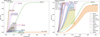Fig. 8 Likelihood P(d < R) of non-detection of binary (left) or planetary mass (right) companions within the cavity of a set of observed transition discs as a function of radius under the hypothesis that companions caus the cavity to form (obtained as described in Sect. 4.2.2). For each system, the plot shows two curves that are joined by a colour-shaded area. The solid curve is associated with the optimistic ($q_{\text{max}}^{+}$, Eq. (8)) companion detection limits, and the dotted curve is associated with the conservative ($q_{\text{max}}^{-}$, Eq. (9)) companion detection limits. The colour-shaded area is a confidence interval between the two upper limits of the mass ratio. The end of each line marks the location of the cavity edge $R=a_{\text{cav}}^{\text{obs}}$. Under the assumption that a companion forms the cavity, P(d < R) represents the likelihood that a companion with a projected separation d < R remains undetected in the disc cavity. For example, for the system CQ Tau, assuming a companion is carving the observed cavity, P(d < R = 0.2) ∼ 80% represents the likelihood that it goes undetected if it has projected separation d < 0.2 arcsec. The value of $P(d<R=a_{\mathrm{c}\mathrm{a}\mathrm{v}}^{\text{obs}})$, that is the value of P at the end of each line, represents the total likelihood in the whole cavity area. We label the total likelihood for the conservative and optimistic upper limits of binaries and planets as ${\mathcal{L}}_{\text{bin}}^{\pm }$ and ${\mathcal{L}}_{\text{pl}}^{\pm }$, respectively, and report them in Table 2. Additional discussion can be found in Sect. 5. As discussed in Sect. 4.2, we remark that a low likelihood allows us to exclude our hypothesis that a companion is responsible for the cavity; in contrast, a high likelihood does not mean that a companion is expected to be found in the cavity, but that under the hypothesis a companion is there carving the cavity high are the chances it goes undetected.

5 Discussion

Fig. 8 shows that the optimistic and conservative upper limits on the mass ratios at various distances from the central star mean that a stellar binary companion is unlikely in 8 of the 13 transition discs that we considered, with a likelihood 0% < ${\mathcal{L}}_{\text{bin}}^{\pm }<30\mathrm{\%}$. This low likelihood, even for the optimistic detection limits, leads us to conclude that undetected stellar binary companions that would carve the cavity can be safely excluded in these systems. However, for 5 systems – AB Aur (for which we could not find mass upper limits), MWC 758, HD 135344B, CQ Tau, and HD 169142 – the optimistic and conservative detection limits both show that a fraction ${\mathcal{L}}_{\text{bin}}^{\pm }>60\mathrm{\%}$ of the configurations of the stellar sample might carve the observed cavity even though they remain undetected. All these systems have been proposed to host planetary or stellar companions – either putative or speculative – within their cavities. (e.g. AB Aur, Poblete et al. 2019; Boccaletti et al. 2020; Currie et al. 2022; MWC 758, Dong et al. 2018; HD 135344B, Stolker et al. 2016, CQ Tau, Ubeira Gabellini et al. 2019; and HD 169142, Fedele et al. 2017; Toci et al. 2020b; Poblete et al. 2022).

In contrast, in all but one system, the majority of companions in the planetary sample would apparently remain undetected. The conservative and optimistic likelihoods both range between $70\mathrm{\%}<{\mathcal{L}}_{\mathrm{p}\mathrm{l}}^{\pm }<100\mathrm{\%}$, including HD 142527, for which, as mentioned above, a putative tertiary planetary companion has been suggested to carve the large cavity. System J1604-2130 instead has a likelihood $28\mathrm{\%}<{\mathcal{L}}_{\mathrm{p}\mathrm{l}}^{\pm }<77\mathrm{\%}$, which makes it less likely that a planet that carves the observed cavity remains undetected, but it remains far from being ultimately ruled out.

In general, we note that the nominal values of the detection limits are sufficiently low to exclude almost any stellar binary companion in regions that were explored through sparse aperture and coronagraph techniques. With the current detection limits, stellar companions are only possible in regions without applied limits because they were covered by the coronagraph and lacked sparse aperture masking limits. In contrast, the available sensitivity is typically only sufficient to detect the most massive planets with M_p ≳ 5−10 M_J, which constitute a small fraction of the planet population we assumed (the masses of ∼ 84% of the planetary sample range between 5 × 10⁻⁴ M_J < M_p ≲ 13 M_J). This leaves many possible planet configurations in the sample that can be hosted in transition discs, but cannot be detected.

6 Caveats and assumptions

The results we presented depend on the choices and assumptions about (i) the planet and stellar binary populations, (ii) the observational upper limits on the companion masses (that might change with future observations), and (iii) the truncation prescriptions.

Concerning (i), more accurate estimates for the planetary and stellar populations can be obtained by refining the distributions we used to generate our samples. The stellar and planetary samples were both generated starting from considerations that are mostly applicable to evolved systems (field binaries and the exoplanet population). Furthermore, the planet distributions were obtained from the raw data in the NASA Exoplanet Archive without accounting for observational biases when extrapolating the properties of the planetary population. Finally, the mutual inclinations between discs and stellar binaries were taken to be randomly oriented for simplicity (uniform distribution of cos (i_d)), while it might be more appropriate to assume a bimodal coplanar/polar distribution for stellar binaries (e.g. Aly et al. 2015; Zanazzi & Lai 2018; Cuello & Giuppone 2019; Martin & Lubow 2019). However, the distributions we adopted constitute a reasonable approximation of the general properties of stellar and planetary populations. To support this statement, as noted in Sect. 4.1, the cumulative distribution of the stellar population in Fig. 7 appears to become progressively similar to the distribution for the planet population for decreasing values of q_max, even though the underlying distributions for e and q are profoundly different. By experimenting with different distributions, we found that the key ingredients for shaping the qualitative behaviour of P(d/a_cav < $\mathcal{R}$) are (i) the value of q_max, (ii) an at least moderate eccentricity for the elements in the sample (e_bin ≳ 0.15), and (iii) the geometric projection in the plane of the sky. For these reasons, we therefore do not expect that a finetuning of the stellar and planetary populations will significantly change our conclusions (although it might be interesting).

Concerning (ii), as discussed in Sect. 4.2, our choices for mass-ratio detection limits for stellar and planetary companions constitute reasonable upper limits based on observations. Future observations are expected to further reduce the P(d/a_cav < $\mathcal{R}$) cumulative likelihood. However, some additional considerations in this regard deserve further discussion. Because the typical q_max ∼ 0.005−0.01, almost any stellar companion would be detected in spatial regions in which these limits apply (R > 0.1^′′)⁷. The stellar companions that survive have projected separations in regions where no limits have been placed because of the coverage of the coronagraph or insufficient resolution. In contrast, cuts with these limits only remove the most massive planetary companions. This issue has the following implications. On the one hand, we do not expect changes in the likelihood for stellar companions unless upper limits become available in currently unexplored regions. On the other hand, the likelihood of planetary companions is not expected to change unless the current detection limits are lowered by a factor 5–10, which implies a q_max ∼ 10⁻³. This would allow the cuts to exclude a larger fraction of the planetary sample. The future advent of the Extremely Large Telescope and observations from the James Webb Space Telescope will enhance the resolution and sensitivity of planet detection campaigns through direct imaging. As a general word of caution, we note that foreground or disc extinction for systems deeply embedded in the cloud (e.g. IRS 48) may reduce the observed luminosity of potential companions, possibly making them not detectable even with the most sensitive instruments.

Concerning (iii), we consider our truncation prescription for the planetary and stellar companions to be reasonable (an additional discussion of how the prescription compares to other results for disc truncation can be found in Appendix D). Fig. 6 shows that the distributions of a_bin/a_cav indicate cavity sizes that typically lie in the range 2 a_bin ≲ a_cav ≲ 4 a_bin for stellar binaries and 1.2 a_bin ≲ a_cav ≲ 2 a_bin for planets. This is perfectly consistent with the extremal values that are typically expected for companions in the mass regime of our populations. In general, prescriptions that predict smaller cavities reduce the likelihood for stellar companions. This does not affect the planetary case strongly because planets would not be detectable in any case unless a significant reduction of q_max also occurs, as discussed above. Similar considerations also apply to the prescription for $a_{\text{cav}}^{\text{obs}}$ = R_mm(1−ϵ), for which a value of ϵ < 25% would further reduce the likelihood. This would again be mostly effective on stellar companions and would be inclined to further reduce the likelihood.

We finally remark that even though P is low, by construction, P(d/a_cav < $\mathcal{R}$) > 0 implies that some companions within the sample that survive after the cuts can in fact carve the observed cavities without being detected. In these cases, the presence of a companion should be considered unlikely, but not impossible. We also note that because binaries spend a very limited fraction of their orbital timescale close to their pericentre, the most compact configurations are relatively short-lived compared to the most extended ones. This was taken into account in the distribution we used to generate the true anomalies. The likelihood is expected to change, however, when more than one observation of the same system is performed after a time frame that permitted the companion to reach a less compact configuration.

7 Conclusion

We presented a novel statistical approach for determining the likelihood that a binary or a planet remains undetected within the cavity of a transition disc under the hypothesis that a companion causes the cavity to form. In this approach, we combined upper limits of companion masses at different locations within the cavity and the probability that each companion is observed with a specific projected separation in the plane of the sky because of its orbital configurations and orientation in 3D space.

To do this, we created two samples, assuming reasonable distributions for the mass and orbital properties of stellar binaries and planets. These samples also accounted for the probability of orbital phases because companions spend more time at the orbit apocentre than at pericentre. We studied the resulting distributions of their projected separations d relative to their semi-major axes a_bin (d/a_bin) and to the cavity sizes a_cav that they are expected to carve if they were surrounded by a protoplanetary disc (d/a_cav). Our conclusions from this analysis are listed below.

(i) The planetary and stellar binary populations both have distributions of d/a_bin that peak at ⟨ d/a_bin⟩ ∼ 1. However, long tails for d/a_bin < 1 and d/a_bin > 1 can be observed in Fig. 4. In general, this implies that some caution is required before the projected separation d of a companion is used as a proxy value of its semi-major axis a_bin.

(ii) A significant fraction of stellar binaries (∼50%) produce cavities with a_cav > 3 d(d/a_cav < 0.3.; see Fig. 7), although for most systems, a_cav ∼ 3 a_bin (see Fig. 6). Similarly, planetary companions have a long tail with a_cav ∼ 3 d(∼ 20%., for d/a_cav < 0.3) of configurations and a maximum likelihood for a_cav ∼ 1.7 d (i.e. d/a_cav ∼ 0.6).

(iii) Based on our statistical study that considered available upper detection limits (see Fig. 8), we conclude that within the cavities of the systems we examined, undetected cavity-carving companions should be considered unlikely in 8 out of 13 systems, with a likelihood ${\mathcal{L}}_{\text{bin}}^{\pm }<30\mathrm{\%}$. This means that ≳ 70% of the companions in the stellar population sample in these 8 systems would be bright and separated enough from the central star to be observationally detected. These 8 systems are: IRS 48 (see footnote⁴ for a word of caution about this system), HD 142527, SR 21, Sz 91, DoAr 44, DM Tau, LkCa 15, and J1604+2130. However, 5 notable exceptions stand out with ${\mathcal{L}}_{\text{bin}}^{\pm }>60\mathrm{\%}$, namely: AB Aur, MWC 758, CQ Tau, HD 135344B, and HD 169142. In these systems, only a few of the possible configurations (≲40% in the worst case) can be ruled out based on the upper limits of companion detection. In contrast, for the planetary sample, undetected planets remain potentially good candidates (${\mathcal{L}}_{\mathrm{p}\mathrm{l}}^{\pm }>80\mathrm{\%}$) to carve the observed cavities of all transition discs except for one. The exception is J1604-2130, which has a likelihood of $28\mathrm{\%}<{\mathcal{L}}_{\mathrm{p}\mathrm{l}}^{\pm }<77\mathrm{\%}$. However, this value of ${\mathcal{L}}_{\mathrm{p}\mathrm{l}}^{\pm }$ implies a moderate likelihood that an undetected planet carved the cavity, although this possibility is far from being ultimately excluded. We recall that for HD 142527, the likelihood refers to the presence of a third companion in addition to the known binary, which has been shown to be too compact to have carved the observed cavity (Nowak et al. 2024). As discussed in Sect. 4.2, we remark that the likelihood we refer to throughout the paper is the likelihood that companions remain undetected within the cavity of transition discs under the hypothesis that a companion carves it. We note that this is different from the probability that a binary or a planet is present within the cavity.

(iv) Since the most compact configurations are short-lived (since they are close to pericentre), the companion might reach a more extended detectable configuration after a relatively short time. Although the likelihood we discussed took the time spent by each binary in different orbital phases into account, it referred to one single observation. Therefore, it might be good to observe the system again after a sufficiently long period of time, which would allow the companion to reach more extended configurations. This would surely increase the detection probability if the sensitivity is adequate to observe it in its new location. We finally remark that a low but not vanishing \mathcal{L}_bin implies that the configurations for cavities are unlikely, but not impossible.

This work constitutes the first systematic statistical approach to evaluating the likelihood that putative companions that carve cavities in transition discs remain undetected. At the time of observations, companions might be found in a configuration with a compact projected separation in the plane of the sky. For this reason, we encourage the community to always rely on a statistical approach that accounts for this possibility before excluding the presence of companions from an observation. This will be particularly relevant with the new detection limits that are provided by the James Webb Space Telescope and the advent of the Extremely Large Telescope.

Acknowledgements

We thank the referee and the editor for their comments. ER thanks Nikolaos Georgakarakos for fruitful discussion about Eq. (5) and orbital stability. ER acknowledges financial support from the European Union’s Horizon Europe research and innovation programme under the Marie Skłodowska-Curie grant agreement No. 101102964 (ORBIT-D). ER also acknowledges the European Southern Observatory for hosting a three-month secondment within the ORBIT-D project, during which part of this project was developed. GL has received funding from the European Union’s Horizon 2020 research and innovation program under the Marie Sklodowska-Curie grant agreement No. 823823 (DUSTBUSTERS) and from PRIN-MUR 20228JPA3A. NC acknowledges funding from the European Research Council (ERC) under the European Union Horizon Europe programme (grant agreement No. 101042275, project StellarMADE). CFM is funded by the European Union (ERC, WANDA, 101039452). Views and opinions expressed are however those of the author(s) only and do not necessarily reflect those of the European Union or the European Research Council Executive Agency. Neither the European Union nor the granting authority can be held responsible for them. This research has made use of the NASA Exoplanet Archive (Fig. 2), which is operated by the California Institute of Technology, under contract with the National Aeronautics and Space Administration under the Exoplanet Exploration Program. Fig. 1 was created using SPLASH (Price 2007). All the other figures were created using matplotlib python library (Hunter 2007).

Appendix A Comparison with van Albada (1968)

In Fig. A.1 we compare our Monte Carlo approach with the analytical calculations of van Albada (1968) for the quantity ⟨log (d/a_bin)⟩ obtained using fixed values of eccentricity. This result is presented here to show that our Monte Carlo approach is equivalent to the purely analytical approach used by van Albada (1968). However, our Monte Carlo approach enables more flexibility in the management of the distributions that generate the sample. Before any consideration about how Fig. A.1 compares with the results discussed in Sect. 2, one should keep in mind that ⟨log (d/a_bin)⟩ ≠ log (⟨ d/a_bin⟩).

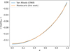Fig. A.1 Comparison of ⟨log(d/a)⟩ from van Albada (1968) (blue curve) and this work (orange). Note that ⟨log (d/abin)⟩ ≠ log⟨(d/abin⟩).

Appendix B Overview of truncation prescriptions

In this section we provide a brief overview of the results concerning tidal disc truncated from binary companions. The semi-major axis of the cavity (or radius if the cavity is circular) a_cav can be predicted analytically, using binary-disc interaction theory, or numerically using hydrodynamical simulations. These latter simulations show that truncation is generally more efficient for dust than for gas, resulting in larger cavities in dust than the corresponding gas features. This is due to the pressureless/inviscid nature of dust grains⁸ and to the dust drift towards gas pressure maxima, which by definition is located at larger radii than the gas truncation radius.

Despite subtle differences among each other, all truncation mechanisms qualitatively share the same dependence on the parameters: the truncation-radius increases with growing e and q of binary (up to q ∼ 0.1, above which a_cav appears to be almost insensitive to the value of q); while it decreases with growing mutual companion-disc inclination i_d, disc aspect ratio H/R, disc viscosity ν.

Such dependences have been thoroughly explored by multiple works that have studied numerically the truncation of dust and gas of circumstellar and circumbinary discs for relatively high binary mass ratios (Pichardo et al. 2005, 2008; Duffell & MacFadyen 2013; Hirsh et al. 2020; Penzlin et al. 2024; Dittmann & Ryan 2024), and for planets with lower mass ratios (Bryden et al. 1999; Crida et al. 2006; Duffell & MacFadyen 2013; Rosotti et al. 2016; Thun et al. 2017; Facchini et al. 2018; Zhang et al. 2018; Chen et al. 2021).

For planetary mass ratios (q < 0.04), despite a large number of numerical simulations in the literature studying eccentric/inclined planet disc interaction (e.g. Goldreich & Sari 2003; D’Angelo et al. 2006; Bitsch et al. 2013; Ragusa et al. 2018; Chen et al. 2021; Baruteau et al. 2021; Zhu & Zhang 2022; Fairbairn & Rafikov 2022; Tanaka et al. 2022; Chametla et al. 2022; Scardoni et al. 2022; Romanova et al. 2024), only Chen et al. (2021) discusses the dependence of truncation (in their case, dust gap width) on planet eccentricity, finding a strong degeneracy between planet mass and its eccentricity, as for higher mass ratios.

Focusing on circular planets, some works (e.g. Rosotti et al. 2016; Facchini et al. 2018; Zhang et al. 2018) found a characteristic relation between the gap width Δ = kR_Hill where R_Hill = a_bin(q/3)^1/3 is the companion Hill’s radius⁹, and k = 4−8 a multiplying factor that depends on the level of coupling between dust and gas and on the degree of evolution of the system (more evolved systems feature wider gaps). In this context, Chen et al. (2021) found that when the planet is eccentric, if the size of the planet epicycle exceeds the Hill’s radius, the epicycle sets the gap width. This implies that the cavity size scales as a_cav = max (1 + Δ, 1 + be), where b is a scale parameter b ∼ k. Systems where more than one planet is present carve a cavity with edge separated by a distance Δ from the outer planet (e.g. PDS 70, Bae et al. 2019).

For stellar binary mass ratios, q ≳ 0.04, two broad categories of truncation prescriptions can be identified: resonant and non-resonant mechanisms (see Appendix C for a thorough discussion). Resonant and non-resonant truncation mechanisms both predict cavity sizes a_cav ∼ 2−4 a_bin, where a_bin is the binary semi-major axis, which are in agreement with typical cavity sizes found in numerical works (e.g. Miranda et al. 2017; Hirsh et al. 2020; Ragusa et al. 2020; Dittmann & Ryan 2024; Penzlin et al. 2024). However, these two truncation mechanisms mainly differ for the fact that the cavity size in resonant mechanisms depends on disc viscosity, while in non-resonant mechanisms it does not depend on the disc properties. In general, resonant theory predicts slightly smaller cavities than non-resonant theory.

Adding to the complexity, numerical studies show that binary/planet-disc interactions can increase the eccentricity of the cavity, which in turn influences its size (e.g. D’Angelo et al. 2006; Kley & Dirksen 2006; Pierens & Nelson 2013; Miranda et al. 2017; Thun et al. 2017; Ragusa et al. 2020; Muñoz & Lithwick 2020; Pierens et al. 2020; Siwek et al. 2023; Toci et al. 2024; Dittmann & Ryan 2024; Penzlin et al. 2024). This result is fully captured within non-resonant orbital stability framework, in a few numerical (Holman & Wiegert 1999; Petrovich 2015; Georgakarakos et al. 2024) and analytical (Shevchenko 2015) studies: in particular, the innermost stable orbit surrounding binaries has a semi-major axis that grows with the test particle eccentricity, thus implying larger cavity sizes for larger cavity eccentricities.

The evolution of disc eccentricity has a complicated dependence on the binary properties (e and q), disc parameters (α−v and H/R; D’Orazio & Duffell 2021; Siwek et al. 2023; Penzlin et al. 2024), self-gravity (e.g. Franchini et al. 2021 finds limited evolution of disc eccentricity in self-gravitating circumbinary discs), and treatment of disc thermodynamics (e.g. Sudarshan et al. 2022). This complex dependence is reflected in observations, where circumbinary discs have been observed to host quite eccentric (e.g. HD 142527; Garg et al. 2021) and also circular cavities (e.g. GG Tau; Toci et al. 2024). Thus, to properly assess the size of the cavity, one should also account for the dependence on the disc eccentricity (e.g. Pierens & Nelson 2013; Petrovich 2015; Ragusa et al. 2020), that can be directly measured observationally through geometric (e.g. Dong et al. 2018) or kinematic (e.g. Garg et al. 2021; Ragusa et al. 2024) considerations.

Appendix C Resonant and non-resonant truncation

As mentioned in Appendix B, binary truncation depends on concurring physical mechanisms that work together to deplete the cavity region: namely, resonant and non-resonant.

In the first (e.g. Goldreich & Tremaine 1980; Artymowicz & Lubow 1994; Miranda & Lai 2015), the gravitational potential of the binary is decomposed into bar-like potentials revolving with pattern frequencies that are integer multiples or rational fractions of the binary one. The main result from studying the perturbative effects of the binary on the disc dynamics is that each term of the expansion of the potential produces a perturbation at a specific radial location in the disc, different for each term of the potential (resonant radii); at these locations, angular momentum and energy are injected into the disc and are transported away through waves. Viscous effects and shock steepening progressively deposit energy and angular momentum in the disc, resulting in an effective torque (Goodman & Rafikov 2001; Crida et al. 2006; Cimerman & Rafikov 2024). Although the deposition of angular momentum and energy can occur relatively far from the resonance where the wave was launched, for non-extreme mass ratios (q > 0.001) of the binary the deposition occurs relatively close to the resonance. By equating the viscous stresses with the resonant flux of angular momentum in the disc, it is possible to define the truncation radius. For this reason, the resonant criterion always predicts truncation at the location of a resonant radius (Miranda & Lai 2015), with abrupt jumps when the tidal torque of the dominant resonance exceeds the viscous one.

In the second, the gravitational perturbations produced by the binary potential cause orbital distortions in the disc orbital motion that result in orbital destabilisation and in the depletion of the disc material (e.g. Papaloizou & Pringle 1977; Paczynski 1977; Pichardo et al. 2005, 2008). At least three separate mechanisms go under the broad category of “non-resonant truncation” mechanisms, each differing in the specific processes responsible for the depletion of the cavity: (i) viscosity dependent tidal torque; (ii) orbital stability; (iii) orbital intersection.

In (i), the perturbation to the disc, due to the summation of all resonant terms in the expansion of the binary potential, produces a tidal wake whose shape depends on the disc viscosity; the wake breaks the axial symmetry and produces a torque on the binary. Vice versa, the binary exerts the same torque on the disc. Since the viscous torque (i.e. the one attempting to close the gap/cavity) and the tidal torque (opening the gap/cavity) both depend on the disc viscosity, the two contrasting open/close torques scale in the same way, resulting in a truncation criterion that is independent of disc viscosity. Although originally predicted as a mechanism for circumstellar disc truncation by Papaloizou & Pringle (1977), the same approach has been used by Artymowicz & Lubow (1994) to calculate the truncation radius of circumbinary discs surrounding circular binaries (e_bin = 0), for which resonant truncation appears to underestimate the cavity size.

In (ii), the perturbative terms in the expansion of the binary gravitational potential produce regions in the binary surroundings where no stable orbits exist (resonance overlap), resulting in the formation of a cavity around the binary. The orbital stability of test particles in a binary potential have been widely studied in the context of the restricted three-body problem from celestial mechanics, identifying regions in space where no stable orbits are allowed surrounding the binary where P-type or S-type circumbinary planets can be found (e.g. Holman & Wiegert 1999; Quarles et al. 2018; Adelbert et al. 2023; Georgakarakos et al. 2024).

Concerning (iii), we first note that orbital stability itself is not sufficient to ensure fluid orbits are not depleted. Indeed, in the proximity of the binary there are regions where stable orbits are possible but intersect other stable outer orbits. When dealing with continuous fluid elements, strong shocks are expected to form in regions with intersecting orbits, depleting the material in the area (Paczynski 1977; Rudak & Paczynski 1981; Pichardo et al. 2005, 2008).

Appendix D Comparison between Pichardo et al. (2005) and the truncation prescription we adopted

Even though the truncation prescription in Eq. (5) has been developed for studying the orbital stability of circumbinary planets and not for disc truncation; we believe it has numerous interesting features that make it particularly suitable for our goal:

1. It reproduces reasonably well the dependence of disc truncation on the binary orbital parameters. This is shown in Fig. D.1, where we compare Eq. (5) with the disc truncation results of Pichardo et al. (2005), with a good level of agreement between the two. The discrepancy results in a reduced chi squared ${\tilde{\chi }}^2\sim 1$, assuming a 12% error bar on all data points, and the worst discrepancy is ∼ 20% for the case e_bin = 0.

2. It offers a straightforward estimate of the truncation radius. In contrast, the resonant approach (e.g. Miranda & Lai 2015) requires numerical solution of complex differential equations. Moreover, since resonant mechanisms rely on the strength of the resonant torque at specific resonant locations, a_cav exhibits a step-like behaviour, with abrupt jumps when the tidal torque exceeds the viscous one.

3. It accounts for the dependence of the cavity size on the mutual binary-disc inclination i_d, and on disc eccentricity e_cav. Although the first has been successfully included in resonant theory (Miranda & Lai 2015), at the moment no works have attempted to include the cavity eccentricity in resonant theory.

4. As previously mentioned, results from non-resonant theory tend to predict slightly larger cavities than those predicted with resonant theory, but do not depend on the disc properties. This implies that Eq. (5) represents a reasonable estimate of the upper limit on the cavity size for each element of the binary sample and will be treated as such when drawing our conclusions.

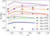Fig. D.1 Comparison between the cavity truncation radii reported in Pichardo et al. (2005) (data points), and the empirical formula by Georgakarakos et al. (2024) in Eq. (5) (solid and dashed lines), for different values of q and ebin. Dashed lines assume ecav = 0, while solid lines use the information about minimum and maximum cavity radii (Rmin, Rmax) provided by Pichardo et al. (2005) to attribute a value of the cavity eccentricity ecav = (1−Rmin/Rmax)/(1+Rmin/Rmax), consistent with the percentage shift of the disc centre from the centre of mass reported in Pichardo et al. (2008). The discrepancy between solid lines and squares results in a reduced chi squared ${\tilde{\chi }}^2\sim 1$, assuming a 12% error bar on all data points, and the worst discrepancy is ∼ 15−20% for the case ebin = 0.

We note that Pichardo et al. (2008) provides a parametric prescription for circumbinary disc truncation obtained interpolating the dataset presented in Pichardo et al. (2005). But, it does not capture correctly the scaling of a_cav for values of 0.01 < q < 0.1, which are outside of the q range simulated in those works. Moreover, the prescription in Pichardo et al. (2008) does not account for the dependence on binary-disc mutual inclination i_d, which is instead the case for the Georgakarakos et al. (2024) one.

Comparison of solid lines with dashed lines in Fig. D.1 suggests that accounting for disc eccentricity e_cav provides a better agreement between data and prescription than e_cav = 0. This result is relevant because a few transition discs have been found to feature eccentric cavities (Dong et al. 2018; Kuo et al. 2022; Garg et al. 2021; Yang et al. 2023).

References

All Tables

All Figures

Fig. 1 Snapshot of a numerical simulation of a circumbinary disc captured in the extreme situation in which the cavity size acav appears to be larger by a factor ∼21 than the apparent separation d of the binary. The snapshot was produced using the code PHANTOM (Price et al. 2018). It shows a binary with a mass ratio M2/M1 = 0.5, semi-major axis abin = 1, and eccentricity ebin = 0.8 close to its pericentre, that is, with a projected binary separation of d ∼ 0.2 abin. The binary produces a cavity with an eccentricity ecav ∼ 0.2 and a semi-major axis acav ∼ 4.2 abin (consistent with the expected truncation radius by such a binary; see Sect. 3.2), which is equivalent to acav ∼ 21 d. The two white dots mark the position of the two binary stars, and the orange and red ellipses show the orbits of the primary and secondary object, respectively. The binary spends far less time at its pericentre than at the apocentre. It is therefore unlikely that the binary is observed in this configuration, but it is still possible.

In the text

	Fig. 2 Probability distributions ${\mathcal{P}}_{e_{\mathrm{p}}}$ (top panel) and ${\mathcal{P}}_{q_{\mathrm{p}}}$ (bottom panel) for the eccentricity e and the mass ratio q of the planet population, respectively.
In the text

Fig. 3 Statistical properties of the samples. Left panel: corner plot distribution of the binary sample we generated for the variables f, e, i, and q for the binary population. Right panel: same as in the left panel, but for the planet population. We deliberately omitted ${\mathcal{P}}_{\varpi }$ because for the binary and planet populations, the longitude of the pericentre ϖ is sampled from a uniform distribution between 0 < ϖ < 2 π. The vertical dashed lines represent intervals containing 16% and 84% of the sample (2σ).

In the text

Fig. 4 Resulting probability density function (pdf) distributions ${\mathcal{P}}_d$ of the quantity d/abin (Eq. (1)), that is, the ratio of the projected separation of the binary d and its semi-major axis abin, for the stellar binary (shaded blue pdf) and planetary population (shaded orange pdf). The probability density value was obtained by binning the values of d/abin and normalising each bin by ni/Ntot Δ xi, where ni is the number of counts in the bin, Ntot is the total number of elements in the sample, and Δ x is the bin size.

In the text

	Fig. 5 Prescription for acav that combines Eq. (5) for q ≥ 0.01 and (6) for q < 0.01. The transition between the two prescriptions at q = 0.01 is smooth. The different colours represent different values of the planet/binary eccentricity. The dotted lines for q < 0.01 are plotted to highlight the transition between the two prescriptions.
In the text

	Fig. 6 Probability density distribution of abin/acav (top panel) and d/acav (bottom panel). The probability density was obtained by binning the values of d/acav and normalising each bin by ni/Ntot Δ xi, where ni is the number of counts in the bin, Ntot is the total number of elements in the sample, and Δx is the bin size.
In the text

Fig. 7 Cumulative distributions P(d/acav < $\mathcal{R}$) calculated using Eq. (7). The solid green and yellow lines show the cumulative distributions for the stellar binary and planetary populations. The dashed lines show distributions obtained by applying a cut q < qmax in the stellar binary regime and renormalising the total distribution to P(d/acav < 1) = 1 to show the impact of q on the cumulative distribution.

In the text

Fig. 8 Likelihood P(d < R) of non-detection of binary (left) or planetary mass (right) companions within the cavity of a set of observed transition discs as a function of radius under the hypothesis that companions caus the cavity to form (obtained as described in Sect. 4.2.2). For each system, the plot shows two curves that are joined by a colour-shaded area. The solid curve is associated with the optimistic ($q_{\text{max}}^{+}$, Eq. (8)) companion detection limits, and the dotted curve is associated with the conservative ($q_{\text{max}}^{-}$, Eq. (9)) companion detection limits. The colour-shaded area is a confidence interval between the two upper limits of the mass ratio. The end of each line marks the location of the cavity edge $R=a_{\text{cav}}^{\text{obs}}$. Under the assumption that a companion forms the cavity, P(d < R) represents the likelihood that a companion with a projected separation d < R remains undetected in the disc cavity. For example, for the system CQ Tau, assuming a companion is carving the observed cavity, P(d < R = 0.2) ∼ 80% represents the likelihood that it goes undetected if it has projected separation d < 0.2 arcsec. The value of $P(d<R=a_{\mathrm{c}\mathrm{a}\mathrm{v}}^{\text{obs}})$, that is the value of P at the end of each line, represents the total likelihood in the whole cavity area. We label the total likelihood for the conservative and optimistic upper limits of binaries and planets as ${\mathcal{L}}_{\text{bin}}^{\pm }$ and ${\mathcal{L}}_{\text{pl}}^{\pm }$, respectively, and report them in Table 2. Additional discussion can be found in Sect. 5. As discussed in Sect. 4.2, we remark that a low likelihood allows us to exclude our hypothesis that a companion is responsible for the cavity; in contrast, a high likelihood does not mean that a companion is expected to be found in the cavity, but that under the hypothesis a companion is there carving the cavity high are the chances it goes undetected.

In the text

	Fig. A.1 Comparison of ⟨log(d/a)⟩ from van Albada (1968) (blue curve) and this work (orange). Note that ⟨log (d/abin)⟩ ≠ log⟨(d/abin⟩).
In the text

Fig. D.1 Comparison between the cavity truncation radii reported in Pichardo et al. (2005) (data points), and the empirical formula by Georgakarakos et al. (2024) in Eq. (5) (solid and dashed lines), for different values of q and ebin. Dashed lines assume ecav = 0, while solid lines use the information about minimum and maximum cavity radii (Rmin, Rmax) provided by Pichardo et al. (2005) to attribute a value of the cavity eccentricity ecav = (1−Rmin/Rmax)/(1+Rmin/Rmax), consistent with the percentage shift of the disc centre from the centre of mass reported in Pichardo et al. (2008). The discrepancy between solid lines and squares results in a reduced chi squared ${\tilde{\chi }}^2\sim 1$, assuming a 12% error bar on all data points, and the worst discrepancy is ∼ 15−20% for the case ebin = 0.

In the text

References

- Adelbert, S., Penzlin, A. B. T., Schäfer, C. M., et al. 2023, A&A, 680, A29 [NASA ADS] [CrossRef] [EDP Sciences] [Google Scholar]
- Alexander, R. D., Clarke, C. J., & Pringle, J. E., 2006, MNRAS, 369, 229 [CrossRef] [Google Scholar]
- Aly, H., Dehnen, W., Nixon, C., & King, A., 2015, MNRAS, 449, 65 [NASA ADS] [CrossRef] [Google Scholar]
- Andrews, S. M., Huang, J., Pérez, L. M., et al. 2018, ApJ, 869, L41 [NASA ADS] [CrossRef] [Google Scholar]
- Artymowicz, P., & Lubow, S. H., 1994, ApJ, 421, 651 [Google Scholar]
- Artymowicz, P., & Lubow, S. H., 1996, ApJ, 467, L77 [NASA ADS] [CrossRef] [Google Scholar]
- Asensio-Torres, R., Henning, Th., Cantalloube, F., et al. 2021, A&A, 652, A101 [NASA ADS] [CrossRef] [EDP Sciences] [Google Scholar]
- Ataiee, S., Pinilla, P., Zsom, A., et al. 2013, A&A, 553, L3 [NASA ADS] [CrossRef] [EDP Sciences] [Google Scholar]
- Bae, J., Zhu, Z., Baruteau, C., et al. 2019, ApJ, 884, L41 [NASA ADS] [CrossRef] [Google Scholar]
- Bae, J., Isella, A., Zhu, Z., et al. 2023, in Inutsuka S., Aikawa Y., Muto T., Tomida K., Tamura M., eds., Astronomical Society of the Pacific Conference Series, 534, Protostars and Planets VII, 423, doi:10.48550/arXiv.2210.13314 [NASA ADS] [Google Scholar]
- Baruteau, C., Wafflard-Fernandez, G., Le Gal, R., et al. 2021, MNRAS, 505, 359 [NASA ADS] [CrossRef] [Google Scholar]
- Biddle, L. I., Bowler, B. P., Zhou, Y., Franson, K., & Zhang, Z., 2024, AJ, 167, 172 [NASA ADS] [CrossRef] [Google Scholar]
- Bitsch, B., Crida, A., Libert, A.-S., & Lega, E., 2013, A&A, 555, A124 [NASA ADS] [CrossRef] [EDP Sciences] [Google Scholar]
- Boccaletti, A., Di Folco, E., Pantin, E., et al. 2020, A&A, 637, L5 [NASA ADS] [CrossRef] [EDP Sciences] [Google Scholar]
- Bryden, G., Chen, X., Lin, D. N. C., Nelson, R. P., & Papaloizou, J. C. B., 1999, ApJ, 514, 344 [CrossRef] [Google Scholar]
- Calcino J., Price D. J., Pinte C., et al. 2019, MNRAS, 490, 2579 [Google Scholar]
- Chametla, R. O., Masset, F. S., Baruteau, C., & Bitsch, B., 2022, MNRAS, 510, 3867 [Google Scholar]
- Chen, Y.-X., Wang, Z., Li, Y.-P., Baruteau, C., & Lin, D. N. C. 2021, ApJ, 922, 184 [NASA ADS] [CrossRef] [Google Scholar]
- Cieza, L. A., González-Ruilova, C., Hales, A. S., et al. 2021, MNRAS, 501, 2934 [Google Scholar]
- Cimerman, N. P., & Rafikov, R. R., 2024, MNRAS, 528, 2358 [NASA ADS] [CrossRef] [Google Scholar]
- Crida, A., Morbidelli, A., & Masset, F., 2006, Icarus, 181, 587 [Google Scholar]
- Cuello, N., & Giuppone, C. A., 2019, A&A, 628, A119 [NASA ADS] [CrossRef] [EDP Sciences] [Google Scholar]
- Currie, T., 2024, RNAAS, 8, 146 [Google Scholar]
- Currie, T., Lawson, K., Schneider, G., et al. 2022, Nat. Astron., 6, 751 [NASA ADS] [CrossRef] [Google Scholar]
- de Juan Ovelar, M., Min, M., Dominik, C., et al. 2013, A&A, 560, A111 [NASA ADS] [CrossRef] [EDP Sciences] [Google Scholar]
- D’Angelo, G., Lubow, S. H., & Bate, M. R., 2006, ApJ, 652, 1698 [CrossRef] [Google Scholar]
- D’Orazio, D. J., & Duffell, P. C., 2021, ApJ, 914, L21 [CrossRef] [Google Scholar]
- Dipierro, G., & Laibe, G., 2017, MNRAS, 469, 1932 [Google Scholar]
- Dittmann, A. J., & Ryan, G., 2024, ApJ, 967, 12 [NASA ADS] [CrossRef] [Google Scholar]
- Dong, R., Liu, S.-Y., Eisner, J., et al. 2018, ApJ, 860, 124 [NASA ADS] [CrossRef] [Google Scholar]
- Duchêne, G., & Kraus, A., 2013, ARA&A, 51, 269 [Google Scholar]
- Duffell, P. C., & MacFadyen, A. I., 2013, ApJ, 769, 41 [NASA ADS] [CrossRef] [Google Scholar]
- Duffell, P. C., & Dong, R., 2015, ApJ, 802, 42 [Google Scholar]
- Dullemond, C. P., Dominik, C., & Natta, A., 2001, ApJ, 560, 957 [NASA ADS] [CrossRef] [Google Scholar]
- Ercolano, B., & Pascucci, I., 2017, Roy. Soc. Open Sci., 4, 170114 [Google Scholar]
- Facchini, S., Pinilla, P., van Dishoeck, E. F., & de Juan Ovelar, M., 2018, A&A, 612, A104 [NASA ADS] [CrossRef] [EDP Sciences] [Google Scholar]
- Fairbairn, C. W., & Rafikov, R. R., 2022, MNRAS, 517, 2121 [Google Scholar]
- Fedele, D., Carney, M., Hogerheijde, M. R., et al. 2017, A&A, 600, A72 [NASA ADS] [CrossRef] [EDP Sciences] [Google Scholar]
- Franchini, A., Sesana, A., & Dotti, M., 2021, MNRAS, 507, 1458 [NASA ADS] [Google Scholar]
- Francis, L., & van der Marel, N., 2020, ApJ, 892, 111 [Google Scholar]
- Garg, H., Pinte, C., Christiaens, V., et al. 2021, MNRAS, 504, 782 [Google Scholar]
- Georgakarakos, N., Eggl, S., Ali-Dib, M., & Dobbs-Dixon, I., 2024, AJ, 168, 224 [Google Scholar]
- Goldreich, P., & Tremaine, S., 1980, ApJ, 241, 425 [Google Scholar]
- Goldreich, P., & Sari, R., 2003, ApJ, 585, 1024 [Google Scholar]
- Goodman, J., & Rafikov, R. R., 2001, ApJ, 552, 793 [NASA ADS] [CrossRef] [Google Scholar]
- Hirsh, K., Price, D. J., Gonzalez, J.-F., Ubeira-Gabellini, M. G., & Ragusa, E., 2020, MNRAS, 498, 2936 [NASA ADS] [CrossRef] [Google Scholar]
- Holman, M. J., & Wiegert, P. A., 1999, AJ, 117, 621 [Google Scholar]
- Huang, S., van der Marel, N., & Portegies Zwart, S., 2024, A&A, 691, A155 [NASA ADS] [CrossRef] [EDP Sciences] [Google Scholar]
- Hunter, J. D., 2007, Comput. Sci. Eng., 9, 90 [NASA ADS] [CrossRef] [Google Scholar]
- Kanagawa, K. D., Tanaka, H., & Szuszkiewicz, E., 2018, ApJ, 861, 140 [Google Scholar]
- Keppler, M., Benisty, M., Müller, A., et al. 2018, A&A, 617, A44 [NASA ADS] [CrossRef] [EDP Sciences] [Google Scholar]
- Keppler, M., Penzlin, A., Benisty, M., et al. 2020, A&A, 639, A62 [NASA ADS] [CrossRef] [EDP Sciences] [Google Scholar]
- Kley, W., & Dirksen, G., 2006, A&A, 447, 369 [NASA ADS] [CrossRef] [EDP Sciences] [Google Scholar]
- Kuo, I. H. G., Yen, H.-W., Gu, P.-G., & Chang, T.-E. 2022, ApJ, 938, 50 [NASA ADS] [CrossRef] [Google Scholar]
- Lambrechts, M., Johansen, A., & Morbidelli, A., 2014, A&A, 572, A35 [NASA ADS] [CrossRef] [EDP Sciences] [Google Scholar]
- Long, F., Pinilla, P., Herczeg, G. J., et al. 2018, ApJ, 869, 17 [Google Scholar]
- Long, F., Andrews, S. M., Vega, J., et al. 2021, ApJ, 915, 131 [NASA ADS] [CrossRef] [Google Scholar]
- Longarini, C., Lodato, G., Bertin, G., & Armitage, P. J., 2023, MNRAS, 519, 2017 [Google Scholar]
- Lynch, E. M., Lovell, J. B., & Sefilian, A. A., 2024, MNRAS, 529, L147 [Google Scholar]
- Martin, R. G., & Lubow, S. H., 2019, MNRAS, 490, 1332 [NASA ADS] [CrossRef] [Google Scholar]
- Miranda, R., & Lai, D., 2015, MNRAS, 452, 2396 [Google Scholar]
- Miranda, R., Muñoz, D. J., & Lai, D., 2017, MNRAS, 466, 1170 [NASA ADS] [CrossRef] [Google Scholar]
- Moe, M., & Di Stefano, R., 2017, ApJS, 230, 15 [Google Scholar]
- Muñoz, D. J., & Lithwick, Y., 2020, ApJ, 905, 106 [CrossRef] [Google Scholar]
- Müller, A., Keppler, M., Henning, Th., et al. 2018, A&A, 617, L2 [CrossRef] [EDP Sciences] [Google Scholar]
- Murray, C. D., & Dermott, S. F., 1999, Solar system dynamics [Google Scholar]
- Nowak, M., Rowther, S., Lacour, S., et al. 2024, A&A, 683, A6 [NASA ADS] [CrossRef] [EDP Sciences] [Google Scholar]
- Offner, S. S. R., Moe, M., Kratter, K. M., et al. 2023, in Inutsuka, S., Aikawa, Y., Muto, T., Tomida, K., & Tamura, M., eds., Astronomical Society of the Pacific Conference Series, 534, Protostars and Planets VII, 275, doi:10.48550/arXiv.2203.10066 [NASA ADS] [Google Scholar]
- Paczynski, B., 1977, ApJ, 216, 822 [CrossRef] [Google Scholar]
- Papaloizou, J., & Pringle, J. E., 1977, MNRAS, 181, 441 [NASA ADS] [CrossRef] [Google Scholar]
- Penzlin, A. B. T., Booth, R. A., Nelson, R. P., Schäfer, C. M., & Kley, W., 2024, MNRAS, 532, 3166 [Google Scholar]
- Petrovich, C., 2015, ApJ, 808, 120 [NASA ADS] [CrossRef] [Google Scholar]
- Pichardo, B., Sparke, L. S., & Aguilar, L. A., 2005, MNRAS, 359, 521 [NASA ADS] [CrossRef] [Google Scholar]
- Pichardo, B., Sparke, L. S., & Aguilar, L. A., 2008, MNRAS, 391, 815 [Google Scholar]
- Pierens, A., & Nelson, R. P., 2013, A&A, 556, A134 [NASA ADS] [CrossRef] [EDP Sciences] [Google Scholar]
- Pierens, A., McNally, C. P., & Nelson, R. P., 2020, MNRAS, 496, 2849 [CrossRef] [Google Scholar]
- Pinilla, P., Flock, M., Ovelar, M. d. J., & Birnstiel, T. 2016, A&A, 596, A81 [NASA ADS] [CrossRef] [EDP Sciences] [Google Scholar]
- Pinilla, P., Tazzari, M., Pascucci, I., et al. 2018, ApJ, 859, 32 [Google Scholar]
- Poblete, P. P., Cuello, N., & Cuadra, J., 2019, MNRAS, 489, 2204 [NASA ADS] [CrossRef] [Google Scholar]
- Poblete, P. P., Cuello, N., Pérez, S., et al. 2022, MNRAS, 510, 205 [Google Scholar]
- Price, D. J., 2007, PASA, 24, 159 [Google Scholar]
- Price, D. J., Wurster, J., Tricco, T. S., et al. 2018, PASA, 35, e031 [Google Scholar]
- Quarles, B., Satyal, S., Kostov, V., Kaib, N., & Haghighipour, N., 2018, ApJ, 856, 150 [NASA ADS] [CrossRef] [Google Scholar]
- Ragusa, E., Dipierro, G., Lodato, G., Laibe, G., & Price, D. J., 2017, MNRAS, 464, 1449 [Google Scholar]
- Ragusa, E., Rosotti, G., Teyssandier, J., et al. 2018, MNRAS, 474, 4460 [CrossRef] [Google Scholar]
- Ragusa, E., Alexander, R., Calcino, J., Hirsh, K., & Price, D. J., 2020, MNRAS, 499, 3362 [NASA ADS] [CrossRef] [Google Scholar]
- Ragusa, E., Fasano, D., Toci, C., et al. 2021, MNRAS, 507, 1157 [NASA ADS] [CrossRef] [Google Scholar]
- Ragusa, E., Lynch, E., Laibe, G., Longarini, C., & Ceppi, S., 2024, A&A, 686, A264 [NASA ADS] [CrossRef] [EDP Sciences] [Google Scholar]
- Regály, Z., Juhász, A., Sándor, Z., & Dullemond, C. P., 2012, MNRAS, 419, 1701 [Google Scholar]
- Regály, Z., Juhász, A., & Nehéz, D. 2017, ApJ, 851, 89 [CrossRef] [Google Scholar]
- Rice, W. K. M., Armitage, P. J., Wood, K., & Lodato, G., 2006, MNRAS, 373, 1619 [Google Scholar]
- Romanova, M. M., Koldoba, A. V., Ustyugova, G. V., Espaillat, C., & Lovelace, R. V. E., 2024, MNRAS, 532, 3509 [Google Scholar]
- Rosotti, G. P., Juhasz, A., Booth, R. A., & Clarke, C. J., 2016, MNRAS, 459, 2790 [Google Scholar]
- Rudak, B., & Paczynski, B., 1981, Acta Astron., 31, 13 [NASA ADS] [Google Scholar]
- Scardoni, C. E., Clarke, C. J., Rosotti, G. P., et al. 2022, MNRAS, 514, 5478 [NASA ADS] [CrossRef] [Google Scholar]
- Shevchenko, I. I., 2015, ApJ, 799, 8 [Google Scholar]
- Shi, Y., Long, F., Herczeg, G. J., et al. 2024, ApJ, 966, 59 [Google Scholar]
- Simon, M., Ghez, A. M., Leinert, Ch., et al. 1995, ApJ, 443, 625 [NASA ADS] [CrossRef] [Google Scholar]
- Siwek, M., Weinberger, R., Muñoz, D. J., & Hernquist, L., 2023, MNRAS, 518, 5059 [Google Scholar]
- Stolker, T., Dominik, C., Avenhaus, H., et al. 2016, A&A, 595, A113 [NASA ADS] [CrossRef] [EDP Sciences] [Google Scholar]
- Stolker, T., Kammerer, J., Benisty, M., et al. 2024, A&A, 682, A101 [NASA ADS] [CrossRef] [EDP Sciences] [Google Scholar]
- Sudarshan, P., Penzlin, A. B. T., Ziampras, A., Kley, W., & Nelson R. P., 2022, A&A, 664, A157 [NASA ADS] [CrossRef] [EDP Sciences] [Google Scholar]
- Tanaka, Y. A., Kanagawa, K. D., Tanaka, H., & Tanigawa, T., 2022, ApJ, 925, 95 [NASA ADS] [CrossRef] [Google Scholar]
- Thun, D., Kley, W., & Picogna, G., 2017, A&A, 604, A102 [NASA ADS] [CrossRef] [EDP Sciences] [Google Scholar]
- Toci, C., Lodato, G., Christiaens, V., et al. 2020a, MNRAS, 499, 2015 [NASA ADS] [CrossRef] [Google Scholar]
- Toci, C., Lodato, G., Fedele, D., Testi, L., & Pinte, C. 2020b, ApJ, 888, L4 [Google Scholar]
- Toci, C., Ceppi, S., Cuello, N., et al. 2024, A&A, 688, A102 [NASA ADS] [CrossRef] [EDP Sciences] [Google Scholar]
- Ubeira Gabellini, M. G., Miotello, A., Facchini, S., et al. 2019, MNRAS, 486, 4638 [NASA ADS] [CrossRef] [Google Scholar]
- van Albada, T. S., 1968, Bull. Astron. Inst. Netherlands, 20, 47 [NASA ADS] [Google Scholar]
- van der Marel, N., 2023, Eur. Phys. J. Plus, 138, 225 [NASA ADS] [CrossRef] [Google Scholar]
- van der Marel, N., Williams, J. P., Ansdell, M., et al. 2018, ApJ, 854, 177 [Google Scholar]
- van der Marel, N., Birnstiel, T., Garufi, A., et al. 2021, AJ, 161, 33 [Google Scholar]
- Wang, J. J., Vigan, A., Lacour, S., et al. 2021, AJ, 161, 148 [Google Scholar]
- Wisdom, J., 1980, AJ, 85, 1122 [NASA ADS] [CrossRef] [Google Scholar]
- Yang, H., Fernández-López, M., Li, Z.-Y., et al. 2023, ApJ, 948, L2 [NASA ADS] [CrossRef] [Google Scholar]
- Zanazzi, J. J., & Lai, D., 2018, MNRAS, 473, 603 [NASA ADS] [CrossRef] [Google Scholar]
- Zhang, S., Zhu, Z., Huang, J., et al. 2018, ApJ, 869, L47 [Google Scholar]
- Zhou, J.-L., Lin, D. N. C., & Sun, Y.-S., 2007, ApJ, 666, 423 [Google Scholar]
- Zhu, Z., & Zhang, R. M., 2022, MNRAS, 510, 3986 [NASA ADS] [CrossRef] [Google Scholar]
- Zhu, Z., Nelson, R. P., Dong, R., Espaillat, C., & Hartmann, L., 2012, ApJ, 755, 6 [Google Scholar]
Even though they also appear to be frequent around less luminous low-mass M-type stars (Shi et al. 2024).
Throughout the paper, we often refer to stellar and planetary companions as “binaries”. We use the term in its broader definition of “two gravitationally bound masses”.
The ratio of the semi-minor and semi-major axes is bcav/acav =  , so that for ecav ≲ 0.3, we obtain bcav ≳ 0.95 acav ∼ Rcav.
For IRS48 (van der Marel et al. 2021) reports a detection limit obtained through lunar occultation from Simon et al. (1995); we report it among the sparse aperture upper limits that are relevant for R < 0.2 arcsec. However, we note that this source is known to be deeply embedded in the cloud, and the conversion from flux sensitivity to mass upper limits might be unreliable (Calcino et al. 2019).
To avoid confusion, we remark that the difference between  and R is that the first is a non-dimensional parameter that compares with d/acav, while R =
acav is in physical units and compares with d.
Obtained using Eq. (5) with q = 0.1, ebin = 0.47, abin = 10.9 au (Nowak et al. 2024), and assuming a circular coplanar orbit of the tertiary companion.
The mass detection limits depend on the model of planet formation that is invoked. The limits reported here are consistent with the lowest end of masses that are detectable with SPHERE M ≳ 5 MJ. For a colder model, the lowest detectable mass would typically reach M ≳ 15 MJ (Asensio-Torres et al. 2021).
Even though Longarini et al. (2023); Lynch et al. (2024) discuss the role of dust pressure.
This relation is in qualitative agreement with the scaling of the width of the spatial region where resonance overlapping produces chaotic orbits in the three body problem (Wisdom 1980), pointing towards a truncation mechanism that appears to be tightly related to orbital stability considerations.
All Tables
Comparison between observational and theoretical acav for a few systems with known orbital properties of the companions.