| Issue |
A&A
Volume 698, June 2025
|
|
|---|---|---|
| Article Number | A6 | |
| Number of page(s) | 19 | |
| Section | Galactic structure, stellar clusters and populations | |
| DOI | https://doi.org/10.1051/0004-6361/202554057 | |
| Published online | 27 May 2025 | |
Stellar-wind feedback and magnetic fields around young compact star clusters: 3D magnetohydrodynamics simulations
Max-Planck-Institut für Kernphysik,
Saupfercheckweg 1,
69117
Heidelberg,
Germany
★ Corresponding author: This email address is being protected from spambots. You need JavaScript enabled to view it.
Received:
6
February
2025
Accepted:
24
March
2025
Abstract
Context. The environments of young star clusters are shaped by the interactions of the powerful winds of massive stars and their feedback on the cluster birth cloud. Several young star clusters show diffuse γ-ray emission on the degree scale, which hints at ongoing particle acceleration.
Aims. To date, particle acceleration and transport in star-cluster environments are not well understood. A characterisation of magnetic fields and flow structures is necessary to progress towards physical models. Previous work has largely focused on 100 pc scale feedback or detailed modelling of wind interaction of just a few stars. We aim to bridge this gap. We focus in particular on compact clusters in order to study collective effects arising from stellar-wind interaction. Objects in this class include Westerlund 1 and R136.
Methods. We performed 3D ideal-magnetohydrodynamics simulations of compact young massive star clusters. We kinetically injected stellar winds for 46 individual very massive stars (M > 40 M⊙) distributed in a spherical region of radius ≤1 pc. We included a sub-population of five magnetic stars with increased dipole field strengths of 0.1–1 kG, and we studied the evolving superbubble over several hundred thousand years.
Results. The bulk flow and magnetic fields show an intricate non-uniform morphology that is critically impacted by the relative position of individual stars. The cluster wind terminates in a strong shock that is non-spherical, and similar to the flow, it has non-uniform properties. The magnetic field is composed of both highly tangled sections and coherent quasi-radial field-line bundles. Steep particle spectra in the teraelectronvolt domain arise naturally from the variation of magnetic field magnitude over the cluster-wind termination shock. This finding is consistent with γ-ray observations. We deem the scenario of petaelectronvolt particle acceleration as unlikely.
Key words: acceleration of particles / magnetohydrodynamics (MHD) / stars: winds, outflows / ISM: bubbles / open clusters and associations: general
© The Authors 2025
 Open Access article, published by EDP Sciences, under the terms of the Creative Commons Attribution License (https://creativecommons.org/licenses/by/4.0), which permits unrestricted use, distribution, and reproduction in any medium, provided the original work is properly cited.
This article is published in open access under the Subscribe to Open model.
Open Access funding provided by Max Planck Society.
1 Introduction
Massive stars feed back onto their environment through powerful winds and ionising radiation. The majority of massive stars live in young star clusters (Higdon & Lingenfelter 2005). The collective feedback from such clusters shapes their local environment and impacts galaxy evolution (see Schinnerer & Leroy 2024). Stellar winds in particular can excavate ambient medium, creating so-called superbubbles, which are filled with hot, tenuous turbulent gas and extend over a scale of 100 pc (see Chu 2008). Superbubbles have been observed, for example, in the 30 Doradus region in the Large Magellanic Cloud (e.g. Townsley et al. 2006). The impact of wind feedback on a galactic scale has been strikingly revealed by recent observations with the James Webb Space Telescope (Lee et al. 2023, and other works published in the same issue). Young star clusters present a diverse source class. They can differ by their extension, stellar composition, and environment. Stellar-wind interaction and feedback depend on these parameters. Compact massive clusters in particular produce powerful winds over a scale of several 10 pc. Such clusters include, for example, Westerlund 1 and R136 (see Portegies Zwart et al. 2010).
In recent years, regions harbouring massive stars have been found to emit γ-rays. In the teraelectronvolt domain, this includes Westerlund 1 (HESS Collaboration 2022), Westerlund 2 (HESS Collaboration 2011), the Cygnus region (LHAASO Collaboration 2024), W43 (LHAASO Collaboration 2025), R136, and 30 Doradius C (HESS Collaboration 2024). Emission from these objects can extend to photon energies ≳100 TeV, typically with steep, curved spectra. In particular, the exceptional detection of petaelectronvolt photons from the Cygnus region raises the question as to which role star-cluster environments play in the Galactic cosmic-ray ecosystem. The isolated supernovae standard paradigm for the origin of Galactic cosmic rays is challenged by several observational facts, such as the anomalous 22N/20Ne ratio (see Gabici et al. 2019; Gupta et al. 2020). This measurement and the recent γ-ray detections, among other considerations, motivate the investigation of non-thermal processes in young star-cluster environments. Furthermore, the galactic-scale feedback from young star clusters impacts particle transport in the galactic disc and escape into the halo. In turn, the physics of the local medium, the dynamics of giant molecular clouds, and galaxy evolution as a whole are affected by the escape of non-thermal particles from their production sites and transport within the Galaxy.
Non-thermal processes in star-cluster environments are sensitive to stellar-wind feedback across several scales, from the sub-parsec range to the scale of the superbubble (100 pc). A number of scenarios for the production of non-thermal particles coexist (e.g. Bykov & Fleishman 1992; Klepach et al. 2000; Ferrand & Marcowith 2010; Gupta et al. 2020; Morlino et al. 2021; Vieu et al. 2022; Vieu & Reville 2023). The parameter space of these models is not well constrained due to the large number of free parameters resulting from the complexity of star-cluster environments and the difficulty of constraining many of these parameters from observations. This concerns, in particular, the cluster-wind termination shock, which has been purported to be a favourable site of particle acceleration (e.g. Morlino et al. 2021). Analytic models for wind interaction in star clusters have been developed in idealised spherically symmetric cases (Chevalier & Clegg 1985; Cantó et al. 2000). Such models do not capture the 3D morphology nor the asymmetries introduced by powerful individual stars, such as Wolf-Rayet (WR) stars. In addition, 1D analytical models do not account for how the magnetic field is shaped by stellar-wind interaction. However, the magnetic fields’ details are of prime importance for the acceleration and confinement of particles in a star-cluster environment. These issues have motivated detailed studies of stellar-wind interaction using numerical simulations. Star cluster feedback has been investigated in a variety of works over the past decades (e.g. Krause et al. 2013; Rogers & Pittard 2013; Gupta et al. 2018; El-Badry et al. 2019; Lancaster et al. 2021). These studies emphasise the superbubble-scale and feedback onto molecular clouds and the interstellar medium. They therefore employed simple wind injection schemes, such as the injection of thermal energy. However, to understand the flow, shock conditions, and magnetic field geometry in the depths of the superbubble, kinetic injection of individual winds is required. In particular, the cluster core must be resolved at sub-parsec scales. This is a challenging task that has only been attempted in a handful of recent works (Badmaev et al. 2022; Badmaev et al. 2024; Vieu et al. 2024a,b), and a comprehensive magnetohydrodynamics (MHD) simulation study including sub-particle to superbubble scales is lacking thus far.
The aim of the present work is to fill this gap. We place particular emphasis on potential particle acceleration sites, such as the cluster-wind termination shock, in order to discuss implications for γ-ray emission. Since our aim is to study collective effects of stellar-wind interaction, we focus on compact clusters. In this context, compact clusters are defined as those in which collective effects are strong enough to produce a cluster-wind termination shock. In loose clusters, such as Cygnus OB2, this is not the case (see Vieu et al. 2024b). The present work is structured as follows: Sect. 2 describes how stars and the cluster are modelled. In Sect. 3 and 4, we describe results concerning the hydrodynamical behaviour and the magnetic field, respectively. Based on our findings, we then discuss particle acceleration and propagation in star-cluster environments in Sect. 5 and conclude with Sect. 6.
2 Setup
Our aim is to investigate stellar-wind interactions around prototypical compact young massive clusters to gain insight into the nature of collective effects therein and how such regions may accelerate particles to high energies. The complementary case of loose clusters was discussed in Vieu et al. (2024b) inspired by the example of the Cygnus star-forming region. We begin with a description of the numerical setup in Sect. 2.1 and then introduce how the star cluster and ambient medium are modelled in Sects. 2.2–2.7. All parameters of our model star cluster are summarised in Table B.1.
2.1 Numerical setup, grid, and outer boundary
We utilised the publicly available finite-volume code PLUTO (Mignone et al. 2007), version 4.4-patch2, to solve the ideal-MHD equations:
![Mathematical equation: $\[\frac{\partial \rho}{\partial t}=-\nabla \cdot(\rho \boldsymbol{u}),\]$](/articles/aa/full_html/2025/06/aa54057-25/aa54057-25-eq1.png) (1)
(1)
![Mathematical equation: $\[\rho\left(\frac{\partial \boldsymbol{u}}{\partial t}+(\boldsymbol{u} \cdot \nabla) \boldsymbol{u}\right)=\nabla \cdot\left(p+\frac{B^2}{8 \pi}\right)+\frac{1}{4 \pi}(\boldsymbol{B} \cdot \nabla) \boldsymbol{B},\]$](/articles/aa/full_html/2025/06/aa54057-25/aa54057-25-eq2.png) (2)
(2)
![Mathematical equation: $\[\frac{\partial \boldsymbol{B}}{\partial t}=\nabla \times(\boldsymbol{u} \times B),\]$](/articles/aa/full_html/2025/06/aa54057-25/aa54057-25-eq3.png) (3)
(3)
where ρ is the mass density, u the velocity, p the pressure, and B the magnetic field vector. We adopted an ideal equation of state with an adiabatic index of 5/3. We choose the TVDLF Riemann solver, second-order Runge-Kutta time-stepping, and linear spatial reconstruction for second-order accuracy in space. The divergence-cleaning algorithm (div_cleaning) is used to enforce the ∇ · B = 0 condition over the course of the simulation. We switch to the entropy equation (Balsara & Spicer 1999) if the flow speed exceeds 2000 km s−1 and the sonic Mach number is >3. This setting is more restrictive than the one employed for the selective entropy switch implemented in PLUTO. Our setting ensures that the deviation from global energy conservation due to the use of the entropy equation stays at the percent level (see Appendix A). The boundary condition on the external domain is set to outflow. Further description of the PLUTO code can be found in the User’s Guide1.
We use a non-uniform Cartesian grid to facilitate both the implementation of individual stellar winds in the core, and the extension of the grid to the scale of the superbubble. In a cube ±1 pc from the centre of the domain, the grid has a uniform resolution of 0.008 pc per cell. At |x|, |y|, |z| >1 pc, the PLUTO stretched grid function is employed to progressively decrease the resolution down to 0.96 pc, individually along each axis. A side effect of this setup is the presence of rectangular-cuboid cells along the coordinate axes at large distances from the core. We verified that these rectangular cells do not significantly affect the flow pattern, by performing a test run of a cluster rotated by 45° along the x, y, and z axes. All simulations have a total of 5123 cells corresponding to a physical width of the domain of 56 pc.
Our setup is tailored to study the cluster wind termination shock region over several hundred thousand years. We chose to invest resources to achieve high cluster core resolution over a large simulation domain and long timescale rather than include additional physical processes, such as radiative losses and thermal conduction. On the investigated timescales, radiative losses are not expected to have a direct impact on the low-density superbubble interior (see Weaver et al. 1977; El-Badry et al. 2019). Previous work on star-cluster wind-interaction has explored the effects of thermal conduction (Badmaev et al. 2022; Badmaev et al. 2024) and found it to smooth structures in the core but not introduce major morphological changes. Some of the impacts of physical processes left out here can be anticipated from simulations of wind interaction at smaller scales (e.g. Mackey et al. 2025, and references therein).
2.2 Ambient medium
The ambient medium is initialised as a homogeneous medium with an ideal equation of state,
![Mathematical equation: $\[p=c_{\mathrm{s}}^2 \frac{\rho}{\gamma},\]$](/articles/aa/full_html/2025/06/aa54057-25/aa54057-25-eq4.png) (4)
(4)
where γ = 5/3 is the adiabatic index. The sound speed is
![Mathematical equation: $\[c_{\mathrm{s}}=15\left(\frac{T}{10^4 \mathrm{~K}}\right)^{0.5}\left(\frac{\gamma}{5 / 3}\right)^{0.5}\left(\frac{\mu}{0.61}\right)^{0.5} \mathrm{~km} \mathrm{~s}^{-1},\]$](/articles/aa/full_html/2025/06/aa54057-25/aa54057-25-eq5.png) (5)
(5)
where 104 K is the temperature assumed for all runs. We assume a fully ionised gas at solar metallicity, resulting in a mean molecular weight of μ = 0.61. The simulation box is permeated by a uniform 3.5 μG magnetic field along the x-direction, which is in the range that is typically expected in the interstellar medium (e.g. Unger & Farrar 2024). The ambient density is 100 cm−3, which is a typical value for giant molecular clouds, but higher than the average density of the interstellar medium. The density mainly acts as a scaling factor for the size of the superbubble. The choice of a high value is necessary to confine the superbubble in the simulation box over the run time of the simulation.
2.3 Star cluster and winds
We generate a synthetic population of 46 stars with masses above 40 M⊙ and simulate their wind feedback for a total time of 390 kyr. Stellar masses are distributed according to the initial mass function dN ~ M−2.3 dM (Kroupa 2002). This represents the high-mass end of a star cluster with a total number of 500 massive stars (M > 8 M⊙) and total mass of 3.5 × 10⁴ M⊙ above 0.4 M⊙.
All stars are initialised on the main sequence. Stellar positions are drawn randomly from a uniform distribution within a sphere of radius Rc. Stellar and wind parameters are assigned based on the mass of the model stars. We initialise the individual stellar winds at terminal velocity, since the smallest simulated scale is 0.008 pc, which greatly exceeds the largest possible stellar radius. For the terminal wind velocity, u∞, and mass-loss rate, we adopt relations by Seo et al. (2018). These relations are based on grid models for stellar evolution by Ekström et al. (2012) and mass-loss predictions by Vink et al. (2001). The terminal wind velocity is set to u∞ = 2.6uesc for O stars above the bi-stability jump (Vink et al. 2001). We only consider stars with M > 40 M⊙, which are well above the bi-stability jump. The mass-loss rate of an O star on the main sequence is (in M⊙ yr−1)
![Mathematical equation: $\[\log _{10} \dot{M}=-3.38 \times\left(\log _{10} M\right)^2+14.59 \times \log _{10} M-20.84,\]$](/articles/aa/full_html/2025/06/aa54057-25/aa54057-25-eq6.png) (6)
(6)
and the wind power is (in km s−1)
![Mathematical equation: $\[\log _{10} L_{\mathrm{w}}=-3.38 \times\left(\log _{10} M\right)^2+14.77 \times \log _{10} M+21.21.\]$](/articles/aa/full_html/2025/06/aa54057-25/aa54057-25-eq7.png) (7)
(7)
The wind velocity is calculated from these two parameters. The mass is in units of solar masses (M⊙). In the main-sequence phase, the wind power of our model cluster is ![Mathematical equation: $\[L_{\mathrm{w}}=0.5 \dot{M} u_{\infty}^{2}= 3 \times 10^{38} \mathrm{erg} \mathrm{s}^{-1}\]$](/articles/aa/full_html/2025/06/aa54057-25/aa54057-25-eq8.png) . The total power of the excluded stars with M < 40 M⊙ is subdominant, 4 × 1037 erg s−1.
. The total power of the excluded stars with M < 40 M⊙ is subdominant, 4 × 1037 erg s−1.
All parameters are kept fixed for the first 200 kyr of the simulation, after which the most massive stars enter a WR phase. Wolf-Rayet stars have exceptionally powerful winds, and in many clusters, they are expected to dominate the wind power (e.g. in Cygnus OB2; see Vieu et al. 2024b). The mass-loss rate and the terminal wind-velocity in the WR phase depend on stellar mass and WR-type (Hamann et al. 2019; Sander et al. 2019). Here, we apply a simple uniform prescription: we increase the main-sequence mass-loss rate by a factor of ten. The first massive star enters the WR phase at 200 kyr. Less massive stars enter the WR phase with a time-delay according to their lifetime, following the prescription of Zakhozhay (2013), whose work is based on Schaller et al. 1992. While the onset time of the WR phase (200 kyr) is much shorter than the expected main-sequence lifetime of a massive star, we show that it is sufficient for the simulation to reach a quasi-stationary state; in other words, no further major morphological changes occur in the flow and magnetic field pattern. Between simulation time 200 kyr and 390 kyr, a total of five stars enter the WR stage.
Our wind model is qualitative, yet is sufficient to explore the phenomenology of wind flows and magnetic fields in and around compact star clusters, in particular with the aim to better understand the physics of wind interactions. More detailed stellar evolution, stellar motion, binary population, supernovae or red supergiants models present opportunities for future work.
2.4 Stellar radius, rotation, and temperature
To implement the magnetic field and the initial conditions in the vicinity of the stars, we required expressions for stellar radii, temperatures, and rotational velocities. We set stellar radii and temperatures based on Eker et al. (2018), employing their mass-temperature and mass-luminosity relations:
![Mathematical equation: $\[\log _{10} T(M)=-0.170 \times\left(\log _{10} M\right)^2+0.888 \times \log _{10} M+3.671,\]$](/articles/aa/full_html/2025/06/aa54057-25/aa54057-25-eq9.png) (8)
(8)
![Mathematical equation: $\[\log _{10} L(M)=\left(2.865 \times \log _{10} M+1.105\right).\]$](/articles/aa/full_html/2025/06/aa54057-25/aa54057-25-eq10.png) (9)
(9)
Here, M is given in M⊙, L in L⊙, and T in K. The relation for T is also used to set the wind sound speed, cs = 31–36 km s−1 for the chosen mass range, set according to Eq. (5) with γ = 1 for isothermal winds. Since there is no clear scaling with M, the value of urot is fixed at 300 km s−1 for all stars (cf. Grunhut et al. 2017), which amounts to 30–50% of the critical velocity for the stellar masses in our cluster.
The threshold mass of the empirical relations given by Eker et al. (2018) is 31 M⊙, due to limited statistics at higher masses. A comparison between the O star calibration by Martins et al. (2005), which is based on an empirical approach and models allowing for states outside of local thermodynamic equilibrium (non-LTE models), yields an overestimation of T and R⋆ by 11% and 14% when using the Eker et al. (2018) relations at 58 M⊙. We note that our model does not require precise values for T and R⋆. The former value influences exclusively the sound speed inside the stellar-wind initialisation region and is only weakly dependent on T. The stellar radius, R⋆, merely acts as a scaling factor on B, as described in Sect. 2.5.
2.5 Stellar magnetic fields
The strength and morphology of the magnetic fields of massive stars are not well constrained, but existing data are consistent with a dipolar field structure and a bimodal field-strength distribution (e.g. Grunhut et al. 2017), where ≲10% of massive stars have a dipolar surface field strength averaging at ~1 kG at the stellar surface, while the remainder of stars have no detectable fields. We set the field strength of these non-magnetic stars to a fiducial value of 10 G, which would be below the detection threshold. In interplay with stellar rotation, the dipolar field results in a Parker spiral (Parker 1958) beyond the Alfvén radius, where the radial and azimuthal components of the field are given as
![Mathematical equation: $\[B_{\mathrm{r}}=B_0(\theta)\left(\frac{R_{\star}}{r}\right)^2,\]$](/articles/aa/full_html/2025/06/aa54057-25/aa54057-25-eq11.png) (10)
(10)
![Mathematical equation: $\[B_{\varphi}=B_0(\theta) \frac{u_{\mathrm{rot}}}{u_{\mathrm{w}}} ~\sin~ \theta \frac{R_{\star}}{r}\left(1-\frac{R_{\star}}{r}\right),\]$](/articles/aa/full_html/2025/06/aa54057-25/aa54057-25-eq12.png) (11)
(11)
assuming the magnetic axis aligns with the axis of rotation. The expressions above depend on B0; the surface magnetic field at the stellar radius, R⋆; the ratio of the rotational velocity at the equator urot to the wind velocity uw; the polar angle, θ; and the radius, r. At the resolution of the simulations presented in this work, the dependence of the surface field on the polar angle, θ, can be approximated as a split monopole. We included a scaling function to smooth the jump at the stellar equator,
![Mathematical equation: $\[B_0(\theta)=B_{\mathrm{s}} \tanh \left(3\left(\frac{\pi}{2}-\theta\right)\right).\]$](/articles/aa/full_html/2025/06/aa54057-25/aa54057-25-eq13.png) (12)
(12)
We caution the reader that our knowledge of stellar magnetism relies on spectroscopic measurements at the stellar surface. Close to the surface, the scaling of the magnetic field with r does not necessarily follow Eqs. (10) and (11). Naively, one would expect B to follow a dipole scaling inside the Alfvén radius. Neither the Alfvén radius in the wind launching region nor the stellar radius corresponding to the measured B0 are well constrained. This introduces significant uncertainty to the overall appropriate scaling. In addition, we have fixed urot = 300 km s−1 for all stars. The known population of magnetic stars shows on average lower urot than non-magnetic stars. For magnetic stars, urot can be as low as a few to a few 10s of km s−1. However, the variation between individual stars is large and some stars have rotational velocities comparable to those typical for non-magnetic stars (e.g. Grunhut et al. 2017). This impacts our setup only as far as it reduces Bφ, which is the relevant component at r ≫ R⋆. Overall, our assumption on stellar magnetic fields is on the optimistic side.
2.6 Initialisation of stellar winds
At the position of each star, we implemented an internal outflow boundary with a radius of five cells, Rb = 0.04 pc, in which we fixed the wind parameters and the magnetic field as described above. Inside the boundary, ρ follows from mass-continuity,
![Mathematical equation: $\[\dot{M}=4 \pi r^2 u_{\mathrm{w}} \rho(r).\]$](/articles/aa/full_html/2025/06/aa54057-25/aa54057-25-eq14.png) (13)
(13)
Outside Rb, parameters are scaled smoothly to their ambient values to avoid discontinuities at initialisation. This procedure was found to reduce artefacts introduced by the initialisation of spherical wind boundaries on a Cartesian grid and increase stability. The density is scaled up to the ambient density, ρamb, with the function
![Mathematical equation: $\[\lambda(r)=\left(1+\frac{r-R_{\mathrm{b}}}{R_{\mathrm{s}}}\right)^\alpha, \text { where } R_{\mathrm{s}}=\sqrt{\frac{\dot{M}}{4 \pi \rho_{\mathrm{amb}} u_{\mathrm{w}}}}.\]$](/articles/aa/full_html/2025/06/aa54057-25/aa54057-25-eq15.png) (14)
(14)
The parameter α ≥ 2 is set by the requirement that the ambient density be reached at a radius Rt = 2Rb from each star. Scaling down the velocity and magnetic field as
![Mathematical equation: $\[u(r)=\frac{u_{\mathrm{w}}}{\lambda(r)},\]$](/articles/aa/full_html/2025/06/aa54057-25/aa54057-25-eq16.png) (15)
(15)
![Mathematical equation: $\[B_{\varphi}(r)=B_{\varphi}\left(R_{\mathrm{b}}\right) \frac{R_{\mathrm{b}}}{r} \sqrt{\frac{1}{\lambda(r)}}\]$](/articles/aa/full_html/2025/06/aa54057-25/aa54057-25-eq17.png) (16)
(16)
ensures continuity and constant sonic and Alfvénic Mach numbers inside Rt. In addition, uw and Bφ are scaled down to ≲10% of their value at the boundary.
Simulation parameters that differ between runs.
2.7 Simulation runs
We consider three clusters with identical stellar content but different spatial distributions, which we term clusters I–III. Table 1 shows an overview of all runs. The cluster radius is 0.6 pc for clusters I and II and 1 pc for cluster III. The high compactness of clusters I and II was chosen to maximise collective effects within the run time of the simulation. The radius of cluster III is representative of, for example, Westerlund 1 and 2 (see Portegies Zwart et al. 2010). As is demonstrated with our results, cluster I/II and III have the same morphological qualities, as do test runs extending the radius to ~2 pc. The behaviour of the clusters studied here can therefore be considered prototypical for young compact clusters. Stellar and wind parameters were chosen as described in Sect. 2.3 and are summarised in Table B.1. By default, five of the 46 stars in each cluster are magnetic with a surface field of 1 kG. For cluster I, we investigate in addition cases of low and high B. In the low B case, magnetic stars have a surface field strength of 100 G instead of 1 kG. In the high B case, we double the number of magnetic stars to 10 stars, but keep the surface field strength of 1 kG. Non-magnetic stars have a 10 G field. Considering the literature, the high and low B scenarios are atypical, but not implausible for individual clusters (see Sect. 2.5).
3 Bubble structure and evolution
Figure 1 shows density slices in a region ±8 pc around the star cluster centre at t ≥ 200 kyr, ≳100 kyr after a supersonic cluster wind first emerges. We identify three main zones: the subsonic cluster core, the supersonic cluster wind, and the subsonic superbubble interior medium (‘core’, ‘cluster wind’, and ‘superbubble’ hereafter). These three regions can be clearly distinguished in a Mach number plot (see Fig. 2a). Cluster wind and superbubble are separated by the cluster-wind termination shock (cluster WTS). We now discuss the formation of these regions and their evolution in detail.
3.1 Formation and evolution of superbubble and cluster wind
Within 1–2 kyr after initialisation, wind bubbles form around individual stars. The shells of these bubbles quickly encounter each other and break apart, forming a single, joint cluster-wind bubble. Yet individual wind termination shocks persist around individual stars (stellar WTSs). Material accumulates downstream of these shocks increasing pressure and density in the cluster core, which eventually launches a cluster wind. In its way out of the core, the wind flow is broken up and redirected by stellar WTSs, resulting in a complex, non-uniform flow morphology. At ~50–100 kyr, the cluster wind becomes supersonic and forms a cluster WTS beyond the core. The system enters a quasi-stationary state with stationary pressure in the core, stable flow geometry and a gradually expanding non-uniform cluster WTS. The size of the superbubble increases in accordance with 1D analytical theory for point-like injection (see Appendix A). Since the system is quasi-stationary, we proceed to the WR phase at 200 kyr, by increasing the mass-loss of the most massive star ten-fold. Up to the end of the simulation at 390 kyr, five more stars enter the WR phase (see Sect. 2.3 for details). Each new WR star modifies the flow and WTS geometry, as the distribution of injected wind power changes. Significant changes can occur within 10–20 kyr (see Fig. 1, panels b–c and e–f). The disruption of the existing structure visibly increases the dynamics of the downstream flow.
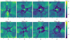 |
Fig. 1 Density slices for cluster I (Rc = 0.6 pc, top) and cluster III (Rc = 1 pc, bottom). The inner ±8 pc are shown, which excludes the superbubble shell. In the left-most panels (a and e), all stars are on the main sequence. The cluster wind is in a quasi-stationary state, slowly expanding over time but not changing geometry. At t > 200 kyr (panels b–d and f–h), the most massive stars consecutively evolve into WR stars. The flow rearranges into a new quasi-stationary state within ~20 kyr after each new WR wind (see panels b–c and e–f). The wind termination shock has a complex, non-spherical geometry, which appears different in different slices (see panels g–h). The white circle in panels g–h indicates the shock radius predicted by 1D analytical theory (Weaver et al. 1977). |
3.2 The central 5 pc: Subsonic core, stellar WTSs, and cluster wind
The star cluster and its immediate environment show stellar winds with Mach numbers >100 embedded in a bulk flow (see Fig. 2a). In the core, where the bulk flow is subsonic, stellar winds form WTSs, whose radii are determined by the balance of stellar wind ram pressure and thermal pressure in core bulk flow (see Dyson & de Vries 1972; Weaver et al. 1977). Material processed through these shocks mixes efficiently before escaping the core as the cluster wind. These findings are in agreement with other work employing 3D simulations to study the core (Badmaev et al. 2022; Badmaev et al. 2024; Vieu et al. 2024a). Stellar winds can also inject material directly into the cluster wind, in particular if they come from a star located at the edge of the cluster. The flow at the contact surface between stellar winds and cluster wind is highly oblique. Material passing this surface mixes less effectively with the bulk flow than it does in the core, which gives rise to density discontinuities extending in the radial direction (e.g. Fig. 1, panels b–c). Some strong winds, such as the WR winds in the present work, fan out and extend all the way to the cluster WTS. We refer to these winds as ‘coupled’ to the WTS. In contrast, stellar winds that are weaker or launched from deeper inside the cluster develop spherical or drop-like shapes. Both a larger separation between stars and a larger asymmetry in the injected wind power decrease the mixing of material into the bulk flow. The core density is on the order of a few particles per cm3 and the density in the wind can drop down to ~3 × 10⁻² cm−3. The cluster WTS Mach number is >5 at 390 kyr of simulation time.
3.3 Transition to subsonic superbubble interior: Cluster WTS and transonic sheets
On the time-frame of our simulations, the cluster wind terminates a few parsec away from the cluster core, producing a boundary layer which is discernible in Figs. 1 and 2 by the jump in density, Mach number, and pressure. We identify this layer as the cluster WTS expected from analytical theory (e.g. Dyson & de Vries 1972; Weaver et al. 1977). As briefly mentioned in Sect. 3.1, the cluster WTS is non-uniform. In particular the Mach number and radius are variable over the surface. The cluster WTS is bent inward by coupled stellar WTSs, giving rise to cone-like structures surrounding the coupled winds, as can be seen in Fig. 3a. The bulk flow is funnelled outward in between the sections dominated by individual stellar winds and eventually becomes shocked and forms sheets (see Figs. 2a and 3b), which can grow to scales of ~10 pc. In these sheets, the flow is compressed along the sheet normal by the pressure in the superbubble and re-accelerates to transonic speeds. In the first ~50–200 kyr, one-dimensional structures can be present in place of sheets, in particular for less dense clusters. These structures, however, do not persist to later times. Embedded within the sheets is a sequence of consecutive shocks, which weaken with increasing distance, the strongest shock being the cluster WTS at the sheet base (see Fig. 2c). This structure resembles ‘shock diamonds’ and recollimation shocks observed in simulations of AGN jets (e.g. Mizuno et al. 2015).
As the cluster WTS expands over time, individual winds can ‘decouple’ and become fully embedded in the cluster wind. This can, though not always immediately, lead to a vanishing of the cone-like structure (see Fig. 1, panels b–c and e–f). The timescale of the decoupling process depends strongly on the distribution of wind power in the cluster, the average distance between stars, and the position of the stars. While the cluster WTS tends to become more spherical over time, it is still visibly asymmetric at the end of our simulation at 390 kyr, despite the rather compact model cluster (compare panels g and h in Fig. 1), indicating that spherical WTSs may be the exception rather than the rule. The cluster I (Rc = 0.6 pc) develops a stronger WTS earlier than cluster III (Rc = 1 pc) and shows a larger fraction of decoupled WTS surface by the end of the simulation. Nevertheless, both models show the same qualitative WTS geometry. In panels g and h of Fig. 1, the cluster WTS radius expected from 1D analytical theory is over plotted. Both panels show the same time, but different slices. The WTS is smaller than expected from 1D theory by ≳50%. This is because the sheets channel the winds’ kinetic energy away from the core, which leads to a less efficient expansion of the cluster WTS.
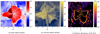 |
Fig. 2 Slices highlighting the properties of shocks in and around the star cluster. (a) Individual stellar winds reach Mach numbers of MS ~ 100 and the cluster wind has MS ~ 10. The transonic sheets, which are found downstream of the cluster-wind termination shock, have MS ~ 1–2. (b) The flow is highly super-Alfvénic, except in a small number of localised regions in the superbubble and cluster core. (c) The cluster-wind termination shock is compressive across its entire surface, as shown by the negative divergence of the velocity field. Alternating compression and rarefaction zones inside the transonic sheets indicate a structure similar to that seen in the ‘shock diamond’ phenomenon. The values have been normalised to the maximum. Panels a and b show a z-axis slice of cluster I at 330 kyr. Panel c shows the same slice at 200 kyr. |
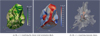 |
Fig. 3 Surfaces of constant sonic Mach number visualising (a) the cluster-wind termination shock and (b) transonic sheets. The two panels in (a) show the orientation of the magnetic field, B (left), and the flow velocity, u (right), with respect to the Mach surface normal, n. In the latter plot, cones (blue, dominated by perpendicular flow) can be clearly distinguished from sheet base shocks (red, inbetween adjacent cones) and coupled stellar winds (red, in the centre of cones). In panel b, the MS = 1 surface is over-plotted onto the MS = 3 surface surface in transparent white, highlighting that sheets extend outward from regions of parallel flow. The panels show cluster I at 390 kyr. |
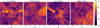 |
Fig. 4 Slices of magnetic field magnitude highlighting the non-uniformity of the field. The non-uniformity can partly be attributed to the five magnetic stars in the cluster. The magnetic field reaches 1 mG in the cluster core and can fall to values of 0.1 μG in the cluster wind. Large asymmetries persist into the superbubble, although they smooth out slowly over time. Two main observations are (1) field amplification behind the wind termination shock (e.g. right-most panel) and (2) mixing of flow from magnetic stars into the bulk medium (e.g. left-most panel). The figure shows data for cluster III sliced along the z-axis. |
4 Magnetic field
We start this section with an overview in Sect. 4.1, illustrating the nature of the magnetic fields. This is followed up by deriving average properties in Sects. 4.2–4.4.
4.1 Qualitative overview
Stars are initialised with randomly oriented Parker spiral magnetic fields. The global magnetic field is determined by how these fields interact, in interplay with the flow. The flow is not magnetically dominated (Alfvénic Mach number MA ≫ 1; see Fig. 2b). Therefore, the flow determines the dynamics of the magnetic field. In ideal MHD, magnetic fieldlines are frozen into the flow. Parker spirals get deformed (e.g. stretched or twisted) as fieldlines are carried in the intricate flow pattern described in Sect. 3. This results in a non-trivial magnetic field morphology, which strongly depends on local wind interactions.
Figure 4 shows the magnetic-field magnitude for cluster III in different regions and at simulation times 200 kyr and 390 kyr. The magnetic field is non-uniform, reaching values of 1 mG close to magnetic stars in the core and dropping to <1 μG in parts of the cluster wind and superbubble. In the superbubble, large patches with comparatively high B can be found where the flow is dominated by winds from magnetic stars. The magnetic field in the core ambient medium is fed by magnetic stars and higher on average than the field in the winds of non-magnetic stars. Asymmetries tend to be smoothed out in the superbubble and B varies on larger spatial scales. We observe magnetic field amplification in the immediate downstream of the cluster WTS.
Figure 5 shows magnetic field streamlines. Close to the cluster (upper panel), the field is highly tangled and locally dominated by Parker spirals from individual stars. The lower panel of Fig. 5 shows that streamlines trace the downstream WTS surface, which is expected from amplification of the perpendicular field component at the WTS. Transonic sheets harbour coherent streamline bundles, extending outward in the radial direction. Coherent streamline bundles are not only found in transonic sheets, but also in coherent subsonic flows, for example, those extending beyond coupled WR winds. Beyond the transonic sheets, the field becomes increasingly disorganised, but all streamlines eventually connect back to the core.
4.2 Average magnitude and distribution
A critical question for particle acceleration and transport is what magnitude B takes in the different regions. We obtain distributions and volume weighted mean and median values of B in the subsonic regions (i.e. the core and superbubble). The volume weighting is necessitated by the non-uniform grid we employ. The values for different regions are computed by filtering based on Mach number and radius.
Figure 6 shows the distributions of B in the core and superbubble for all simulation runs. The mean, median, 25th, and 75th percentiles are marked. All distributions show a tail at large values, in other words, the mean consistently lies above the median. The most skewing is seen in the core, where the magnetic fields are kept fixed inside the stellar boundaries. The least skewing is seen in the bubble, indicating that averaging effects take place. The mean of B lies between 30–200 μG in the core and 5–25 μG in the superbubble. The median values of B are 8–35 μG in the core and 4–20 μG in the superbubble. We note that the flow in both the core and the superbubble is turbulent. By construction, we can only investigate the field modes above the grid resolution. The grid resolution is non-uniform, due to the stretched grid we employ. This leads to a suppression of B in small-scale modes in the superbubble.
In the core, the distribution of B shows noticeable variations between cluster I–III, despite their identical magnetic star content. In contrast to cluster I, cluster II shows clear bimodality at 200 kyr, even though both clusters have identical radii. This indicates that the distribution of B is influenced significantly by local wind interactions. The most powerful magnetic star is located close to the cluster centre for cluster II, while it is closer to the outskirts in cluster I (see Fig. B.1 in Appendix B). The larger B in cluster II could therefore be a consequence of increased mixing of magnetic wind material into the core bulk medium. In the superbubble, cluster II also shows a distribution shifted to higher B at 200 kyr, but shows a distribution equivalent to those of clusters I and III at 390 kyr. This suggests that the distribution of B in the superbubble is not influenced by the efficiency of mixing processes in the core after a few 100 kyr.
Since the superbubble is not a stationary system, median B is not stationary. Before the WR onset, the decrease in the B median values is on average consistent with that expected from the increase in superbubble volume, assuming that magnetic energy is diluted by the expansion of the bubble. After the WR onset, the observed decrease exceeds the one expected from superbubble expansion alone by a factor of about two. All WR winds originate from non-magnetic stars. Therefore, the average wind magnetisation goes down in the WR phase, which can contribute to decrease B.
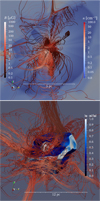 |
Fig. 5 Streamlines of the magnetic field coloured by magnitude. In the upper panel, streamline seed points are placed within the radius of the star cluster. This highlights the tangled morphology arising from the interaction of Parker spiral stellar magnetic fields. The lower panel shows streamlines for a seed point radius comparable to the size of the cluster-wind termination shock (5 pc) over-plotted onto the surface where the sonic Mach number equals three. The surface colour shows the orientation of the flow velocity, u, with respect to the surface normal, n. We note the quasi-radial streamline bundles, which are dragged outward by coherent flows. Such flows are present, for example, in transonic sheets (see Fig. 3b). The figure shows cluster I at 390 kyr. |
4.3 Radial profile
In Sect. 3, several distinct domains were identified, including the subsonic core bulk flow, stellar winds, the cluster wind, transonic sheets, and the subsonic superbubble medium. We obtain radial profiles of the mean magnitude of the magnetic field, ⟨B⟩, in these regions by filtering on the Mach number. The radial profiles are obtained by averaging over a large number of line-outs (10 000). We note that the variation between single line-outs is large (see the large variations in Fig. 4).
Figure 7 shows the radial profile of ⟨B⟩ for cluster II before the WR phase at 200 kyr and 390 kyr. Radial profiles for the remaining simulation runs can be found in Appendix C. At 390 kyr, the radial domain can be broadly sub-divided into a region dominated by the subsonic core medium, a region dominated by supersonic wind, and a region dominated by the subsonic superbubble medium. The transition between the first two is at ~0.8 pc, and between the latter two, it is at 2–3 pc for a cluster radius of 0.6 pc. We note that B decreases slightly steeper than r−1 in the region dominated by supersonic cluster wind. Outside the wind dominated region, it approaches a constant value.
Stellar winds (MS > 20) show values below the overall average by a factor 20–30 and a peak at ~0.6 pc, which is traced by a peak in the subsonic profile. The peak in the stellar wind profile stems from the distribution of magnetic stars. The sharp decline following the peak is an averaging effect: wind from magnetic stars skew the average upward, but contribute only in a narrow range of radius. Only WR winds, which are all non-magnetic, extend out to larger radii. The fact that the peak is traced by the subsonic profile indicates that magnetic stars contribute substantially to the magnetisation of the core bulk medium and cluster wind.
Transonic sheets have ⟨B⟩ close to the overall average at 200 kyr and ⟨B⟩ below the average by about a factor of two at 390 kyr. Before the WR phase, all profiles are shifted to higher ⟨B⟩ values, in line with what was discussed for the B distributions in the preceding section. In addition, a larger fraction of the cluster wind is still in the transonic regime (3 > MS > 1; see Fig. 7).
4.4 Streamline diffusivity
As discussed in Sect. 4.1, the magnetic field shows both tangled sections and coherent structures, such as spirals, loops, and field-line bundles. No simple description for this highly intricate morphology can be provided. Here, we investigate streamline diffusivity to provide a measure for the average behaviour of the field. It also has implications for particle transport, a discussion of which follows in Sect. 5. The streamline diffusivity is defined here as D = ⟨Δx2⟩/2s, where Δx is the spatial separation of two points on a streamline and s the distance along the streamline. We note that, in general treatment, D is a tensor often expressed in terms of components parallel and orthogonal to a local mean field. Since the mean field is not well defined here, we resort to the above scalar definition. We integrate streamlines using Paraview, distributing 1000 streamline starting-points (seeds) uniformly inside a spherical region centred on the star cluster. We investigate three different seed cloud radii (0.6 pc, 2 pc, and 5 pc), corresponding to the size of the cluster core, cluster wind, and cluster WTS regions.
Figure 8 shows the diffusivity at 200 and 390 kyr. We compare clusters I–III. Over all runs and timesteps, the diffusivity is in the range of D = ⟨Δx2⟩/(2s) ~ 0.5–2 pc. Thus, the linear distance is
![Mathematical equation: $\[\Delta x=\left(\frac{D}{0.5 ~\mathrm{pc}}\right)^{0.5}\left(\frac{s}{1 ~\mathrm{pc}}\right)^{0.5} \mathrm{pc},\]$](/articles/aa/full_html/2025/06/aa54057-25/aa54057-25-eq18.png) (17)
(17)
from which it follows that on distances larger than a parsec, fieldline diffusion can play an important role in particle transport. The diffusivity is approximately constant for seeds placed in the core and wind, with some deviation for cluster III at 200 kyr and cluster I at 390 kyr. For a seed cloud radius of 5 pc, the diffusivity is clearly increasing with s, although at 200 kyr, it levels off starting at around 10 pc. This is due to the fact that streamlines reach the edge of the superbubble and loop back to the core. Since the superbubble is larger at 390 kyr, this levelling-off starts at a larger s. The close-to-linear increase prior to this comes from coherent field-line bundles extending outward in transonic sheets. Linear behaviour is expected if streamlines are straight lines. Between 200 kyr and 390 kyr, diffusivity has decreased for cluster III (Rc = 1 pc), while the opposite is true for cluster I (Rc = 0.6 pc). Jointly with the variation between cluster I and II, which only differ by the spatial distribution of stars, this indicates the importance of local wind interactions for the diffusivity. Nevertheless, the difference does not exceed a factor of a few.
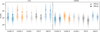 |
Fig. 6 Magnetic field in the cluster core (left) and superbubble interior (right). Triangles mark distributions before the WR onset at 200 kyr, and circles indicate distributions after the WR onset at 390 kyr. Colours indicate different simulation runs (see Table 1 for run parameters). Filled markers show the mean, empty markers the median. Whiskers indicate the 25th and 75th percentiles. Asymmetries due to local wind interactions are larger in the core, as evident by the broader distributions, but are reduced when the flow reaches the superbubble. We note that the distributions are shown in log space. |
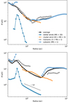 |
Fig. 7 Radial profiles of the mean magnitude of the magnetic field, ⟨B⟩, in different regions for cluster II. The upper panel shows the profiles at 200 kyr, and the lower panels shows them at 390 kyr. The profiles were obtained by averaging over 10 000 randomly drawn line-outs. Points are only plotted where at least 10% of line-outs pass through the indicated region. ⟨B⟩ scales approximately as r−1 in the supersonic cluster wind. The hump in the stellar winds profile close to 0.6 pc stems from magnetic stars and is traced by a hump in the subsonic core medium. This indicates that wind material from magnetic stars significantly increases the magnetisation of the bulk. |
5 Implications for particle acceleration and transport
The results discussed in Sects. 3 and 4 present favourable conditions for particle acceleration at stellar and cluster WTSs within the framework of diffusive shock acceleration (DSA, Axford et al. 1977; Krymskii 1977; Bell 1978; Blandford & Ostriker 1978). In the discussion to follow, we assume that DSA operates at maximum efficiency. In such cases, the maximum particle energy is predicted to be close to the Hillas limit: Emax = ZeBru/c, where q = Ze is the charge of the accelerated particle, u the flow speed, B the magnetic field and r the size of the accelerator (see Lagage & Cesarsky 1983; Hillas 1984). We discuss acceleration at individual stellar WTSs and the cluster WTS in turn in Sects. 5.1 and 5.2. In Sect. 5.3, sub-grid effects and their potential impacts are examined. We then discuss a toy model for the spectrum in Sect. 5.4 and finally turn to particle transport in Sect. 5.5.
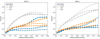 |
Fig. 8 Streamline diffusivity for seed points placed within spheres of the indicated radii at 200 kyr (left) and 390 kyr (right). Triangles, circles, and squares indicate clusters I, II, and III, respectively. The near linear increase for the 5 pc seed cloud radius is due to quasi-radial field-line bundles embedded in transonic sheets (cf. Fig. 5, lower panel) and the levelling-off is due to fieldlines travelling close to the superbubble edge looping back to the core. The variation between clusters I and II, which only differ in the spatial distribution of stars, illustrates the importance of local wind interactions. |
5.1 Acceleration at stellar WTSs in the core
Stellar WTSs in the core have radii of about 0.03–0.3 pc and are strong shocks, MS ≫ 10 (see Fig. 2a). Vieu et al. (2024a) discussed collective effects in the core, and concluded that they do not increase the maximum energy, nor have a significant impact on the spectrum in all considered scenarios. This is mainly because the volume filling factor of the powerful winds in the core is rather small, even for compact clusters, which does not allow particles to interact with multiple shocks within their (short) advection time out of the core. Stellar WTSs in a cluster can therefore be viewed as independent, individual accelerators. The magnetic field in the upstream of individual stellar WTSs is a Parker spiral by initialisation (see Eqs. (10) and (11)). The azimuthal component, Bφ, dominates far from the stellar surface, r ≫ R⋆. Since, in the Hillas limit, Emax ∝ Br, but Bφ ∝ r−1 for a Parker spiral, Emax can be expressed in terms of the surface field, B0. For fiducial parameters of a magnetic star, this gives
![Mathematical equation: $\[E_{\max }<21 \times Z\left(\frac{B_0}{1 ~\mathrm{kG}}\right)\left(\frac{R_{\star}}{10 ~\mathrm{R}_{\odot}}\right)\left(\frac{0.01}{u_{\mathrm{rot}} / u_{\mathrm{w}}}\right)\left(\frac{u_{\mathrm{w}}}{3000 \mathrm{~km} \mathrm{~s}^{-1}}\right) \mathrm{TeV}.\]$](/articles/aa/full_html/2025/06/aa54057-25/aa54057-25-eq19.png) (18)
(18)
Here, the ratio urot/uw enters through Bφ. Standard stars (B0 = 10 G) in our model cluster have Emax < 2.5–5.4 TeV, and magnetic stars (B0 = 1 kG) have Emax < 240–450 TeV. The latter constraint should be taken as being optimistic since we set urot = 300 km s−1 for all stars and the magnetic field possibly scales down steeply close to the stellar surface (see Sect. 2.5). Even in the exceptional case of a high surface field and fast rotation, Emax is limited by the fact that DSA requires an Alfvénic Mach number MA ≫ 1. This places an absolute limit on the maximum energy. With MA = uw/uA, where ![Mathematical equation: $\[u_{\mathrm{A}}=B / \sqrt{4 \pi \rho}\]$](/articles/aa/full_html/2025/06/aa54057-25/aa54057-25-eq20.png) , and the density falling off as
, and the density falling off as ![Mathematical equation: $\[\rho=\dot{M}\left(4 \pi r^{2} u_{\mathrm{w}}\right)^{-1}\]$](/articles/aa/full_html/2025/06/aa54057-25/aa54057-25-eq21.png) , we obtained
, we obtained
![Mathematical equation: $\[\begin{aligned}& E_{\max } \ll 220 \times Z\left(\frac{\dot{M}}{10^{-6} ~\mathrm{M}_{\odot} ~\mathrm{yr}^{-1}}\right)^{0.5}\left(\frac{u_{\mathrm{w}}}{3000 \mathrm{~km} \mathrm{~s}^{-1}}\right)^{1.5} \\&\qquad\qquad\qquad\qquad\qquad\qquad\qquad\qquad \times\left(\frac{M_{\mathrm{A}, \min }}{3}\right)^{-1} \mathrm{TeV},\end{aligned}\]$](/articles/aa/full_html/2025/06/aa54057-25/aa54057-25-eq22.png) (19)
(19)
where we impose a minimum Alfvénic Mach number, MA,min, of three. For stars in our model cluster, the above limit is 100–330 TeV in the main-sequence phase and 1.7 PeV for the most powerful WR star.
In conclusion, the WTS of a typical massive star is not expected to accelerate particles to energies beyond ~10 TeV. Higher energies can only be reached by magnetic stars with B ≳ 100 G, which make up ≲10% of O stars (see Grunhut et al. 2017). Even a fast rotating strongly magnetic star, a case which is both observationally and theoretically expected to be exceptionally rare, can reach at most ~1 PeV. An additional aspect of particle acceleration at stellar WTSs is that the shock is expected to be highly oblique in B, since the Bφ component dominates at the WTS. The implications of magnetic-field obliquity on particle injection efficiency and maximum energy are not fully conclusive (e.g. Bell et al. 2011; Xu et al. 2020; Kumar & Reville 2021).
5.2 Acceleration at the cluster WTS
The cluster wind terminates at a non-uniform shock surface beyond the core, which is made up of coupled stellar WTSs, sheet base shocks, and cones (see Sect. 3.3). The discussion in the preceding section also applies for coupled stellar WTSs. Their surface is larger than that of stellar WTSs in the core. In Emax, however, this is compensated by the fact that B is scaled down to a lower value (B ∝ r−1 approximately; see Fig. 7).
The discussion to follow focuses on the collective part of the cluster WTS, which has MS ~ 10 (see Fig. 2a). We extract properties at sheet bases and cones along 10 000 randomly drawn radial line-outs. The immediate shock upstream is taken to be the location where MS is maximal. Sheet bases and cones differ in the obliquity of the flow (see Fig. 3a). We take the field of normal vectors of the cluster WTS surface to be n = −∇MS/|∇MS|. A threshold of u · n/|u| > 0.7 was found to reliably filter for line-outs passing through sheet bases. The inverse filter identifies cones. Coupled stellar winds are removed by imposing MS < 20. The high obliquity of the flow in cones calls for a verification that they can be considered shocks as opposed to shear layers. The ratio ℛ = ∇ · u/∇ × u quantifies the relative contribution of compression and shear. Less than 1% of line-outs have |ℛ| < 1 in the downstream of the cones for all simulation runs. In addition, the divergence of u shows similar values across all parts of the cluster WTS (see Fig. 2c), with only slightly lower values in the cones.
Figure 9 shows the immediate upstream distribution of a selection of parameters for cluster I at 390 kyr. The sonic Mach number is characterised by a symmetric distribution with median values of about 10 in sheet bases and 9 in cones and MS ≳ 5 everywhere, indicating strong shocks with a compression ratio q > 3.5. The median value of B is 0.5 μG in sheet bases and 0.6 μG in cones. The distribution of log10 B shows a hint of bimodality, with the second mode peaking at about 10 μG. An examination of the distribution of magnetic field values on the cluster WTS surface reveals that values above about 3 μG almost exclusively appear in the flow-paths of magnetic stars. In these regions, upstream values can reach averages of about 20 μG over 1 pc. We note that cluster II shows a significantly lower maximum B in the upstream of sheet base shocks (see Fig. C.1). The fact that the most powerful magnetic star is positioned closer to the centre of the cluster seems to increase the level of mixing, leading to a higher average B (see Fig. 6), but fewer high B outliers. The third panel in Fig. 9 shows the flow speed across the shock, u · n. The speed across the shocks is significantly lower in the cones than it is in the sheet bases, where the modes of the distributions are at about 1400 km s−1 and 2600 km s−1, respectively. The latter value is close to the median magnitude of the velocity, u, which is about 2800 km s−1, with a width of ±50 km s−1 at half maximum. Both distributions are rather broad and show a tail at low values. These tails are due to contamination of the sample with downstream values and the rotation of ∇MS in the numerically smoothed shock. We use ∇MS to determine the shock normal vector. The right-most panel shows that the orientation of B in the shock upstream is highly variable. The median value lies close to 0.4 for both cones and sheet bases.
Thus far, we have demonstrated that both cones and sheet bases are strong shocks with a median upstream magnetic field of 0.5 μG, a broad range of obliquities in B, and lower flow speed normal to the surface in the case of the cones, owing to the obliquity of the flow. Despite these topological subtleties, DSA is expected to take place at both cones and shear bases. The acceleration properties, however, depend on the local parameters of the flow and magnetic field. In the following, the maximum particle energy is estimated case by case. The width of sheet base shocks is d ~ 0.5–3 pc, with a typical value of 1 pc. The median value of 0.5 μG gives
![Mathematical equation: $\[E_{\max }^{\text {sheetbase }}=4.0 \times Z\left(\frac{B}{0.5 ~\mu \mathrm{G}}\right)\left(\frac{d}{1 ~\mathrm{pc}}\right)\left(\frac{u}{2600 \mathrm{~km} \mathrm{~s}^{-1}}\right) \mathrm{TeV}.\]$](/articles/aa/full_html/2025/06/aa54057-25/aa54057-25-eq23.png) (20)
(20)
The cones reach a size comparable to the overall extent of the cluster WTS, which is about 5 pc. The decreased normal flow velocity gives a comparable limit:
![Mathematical equation: $\[E_{\max }^{\text {cones }}=11 \times Z\left(\frac{B}{0.5 ~\mu \mathrm{G}}\right)\left(\frac{d}{5 ~\mathrm{pc}}\right)\left(\frac{u}{1400 \mathrm{~km} \mathrm{~s}^{-1}}\right) \mathrm{TeV}.\]$](/articles/aa/full_html/2025/06/aa54057-25/aa54057-25-eq24.png) (21)
(21)
Since the distribution of B is rather broad, Emax can reach higher values in some regions. In the isolated regions where the field is about 20 μG over 1 pc, Emax is ≲170 TeV. We note that the constraints on Emax are not expected to change considerably when the WTS evolves over a time longer than that covered by the simulation. In the limit of a fully spherical cluster WTS and radial cluster wind, u across the shock is given by the median magnitude, 2800 km s−1, and d is the size of the cluster WTS. This increases Emax by a factor two compared to the limit in the cones. The expansion of the cluster WTS over time does not per se increase Emax, since B drops in the cluster wind approximately as r−1 (see Fig. 7). As a consequence, in Emax, the increase in size of the accelerator cancels with the decrease in B.
In this and the preceding section, we have discussed Emax at stellar WTSs and the cluster WTS, informed by our simulations. We find that Emax does not exceed a few tens of teraelectronvolts in typical scenarios, even when extrapolating our results to a quasi-spherical cluster WTSs grown to several ten parsecs over a timescale of millions of years. Regions of the cluster WTS with higher than average B, for example in the flow-paths of magnetic stars, reach at most a few hundred teraelectronvolts. Individual magnetic stars are unlikely to accelerate particles to these energies (see Eq. (18)) and in fact have a theoretical upper bound on Emax close to 200 TeV for typical parameters. We note that we purposefully left out a discussion of supernovae. The supernovae expanding in the collective wind of a compact cluster can potentially reach higher energies than the cluster WTS (Vieu & Reville 2023). A dedicated analysis of the evolution of supernovae in a star-cluster environment is necessary to assess the properties of acceleration at their shocks.
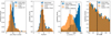 |
Fig. 9 Properties in the immediate upstream of sheet base shocks and wind cones at 390 kyr of simulation time. The histograms were compiled from values along 10 000 randomly drawn line-outs. The distribution of values at sheet bases and cones is similar for most parameters, except the velocity across the shock, u · n (panel 3). (For further description, see the text.) |
5.3 Sub-grid effects
In this section, we explore two mechanisms to generate a magnetic field on sub-grid scales, which could ultimately facilitate acceleration to higher energies than estimated in the two preceding sections: sub-grid dynamos in Sect. 5.3.1 and magnetic field excitation by streaming instabilities in Sect. 5.3.2.
5.3.1 Dynamos
The maximum energy at the cluster WTS is most decisively set by B. We find a typical upstream value of ~0.5 μG. This value is set by the value of B in the core and its scaling in the supersonic cluster wind. A higher Emax at the cluster WTS could therefore be facilitated by a higher B in the core. Even considering that limitations inherent to the numerical approach could affect our measured B, the scaling is always expected to be r−1 or steeper (see Sects. 4.3 and 5.1). In an optimistic scenario (d = 5 pc and u = 2800km s−1), an upstream value of 30 μG could facilitate acceleration to petaelectronvolt energies. This would require a bulk magnetisation in the core of at least 150 μG, assuming the field scales as r−1 in the cluster wind and disregarding potential amplification by streaming instabilities. In our simulation, the magnetisation of the bulk flow in the core is modest, with typical values of 8–35 μG. In principle, dynamo effects below the grid scale (0.008 pc in the core) could increase the value of B. However, dynamo effects would have to amplify B by a factor 5–20 over the simulation value to reach the 150 μG. In conclusion, small scale (<0.01 pc) dynamo effects would have to be by far the dominant effect supplying the magnetic field to facilitate particle acceleration to petaelectronvolt energies at the cluster WTS.
5.3.2 Self-excited magnetic fields
The magnetic-field profiles that emerge from the simulations are inevitably smooth on the grid scale. However, scattering of non-thermal particles is dominated by magnetic-field structures with length scale close to gyro-scale of the particles in question: λ ~ rg ~ EPeVBμG pc. Since the grid resolution in the vicinity of the WTS is of the order 0.1 pc, it is clear that a sub-grid model for self-excited magnetic field fluctuations is needed for particles with energies of interest in this work. In determining the maximum energy at each shock we have made the assumption that DSA operates at maximum efficiency. This entails the implicit assumption of Bohm diffusion, which demands the generation of self-excited MHD modes. To motivate this, we investigate which cosmic-ray driven instabilities can operate, and to what level we might expect the fields to grow/saturate.
The two most commonly invoked processes for self-excitation of scattering fields for energetic cosmic rays are the resonant streaming instability (e.g. Wentzel 1974) and the non-resonant hybrid instability (Bell 2004, 2005). We note that the resonant instability (RSI) has largely only been studied in the context of quasi-parallel shocks, which as we demonstrated applies only in a limited range of the available shock surface. Meanwhile, the non-resonant instability (NRI) can operate at all possible obliquities, though only acts if the cosmic-ray currents can overcome the magnetic field tension at all resonant scales. This condition can be expressed as (Bell 2004; Reville et al. 2021)
![Mathematical equation: $\[\chi=\frac{P_{\mathrm{cr}}}{\rho u^2} \frac{u}{c} M_{\mathrm{A}}^2 \gg 1,\]$](/articles/aa/full_html/2025/06/aa54057-25/aa54057-25-eq25.png) (22)
(22)
which is easily satisfied for the typical conditions found in our simulations: Bbg = 0.5 μG, u = 3000km s−1, n = 0.05 cm−3, and χ ~ 103(Pcr/ρu2). Estimates can be found in the literature for the saturated magnetic field associated with the RSI (e.g. Bell & Lucek 2001; Amato & Blasi 2006) and the NRI (e.g. Bell 2004; Matthews et al. 2017),
![Mathematical equation: $\[\frac{\delta B_{\mathrm{sat}}^2}{4 \pi} \approx\left\{\begin{array}{cc}2 \eta_{\mathrm{cr}} M_{\mathrm{A}} \frac{B_{\mathrm{bg}}^2}{4 \pi} & \text { RSI },\\\eta_{\mathrm{cr}} \rho u^2 \frac{u}{c} & \text { NRI}\end{array}\right.\]$](/articles/aa/full_html/2025/06/aa54057-25/aa54057-25-eq26.png) (23)
(23)
where Bbg is the background field and ηcr = Pcr/ρu2 is the acceleration efficiency, which is typically thought to be about 10%. Numerically, we can express the above as
![Mathematical equation: $\[\delta B_{\mathrm{sat}} \approx\left\{\begin{array}{r}10\left(\frac{B_{\mathrm{bg}}}{1 ~\mu \mathrm{G}}\right)^{1 / 2}\left(\frac{u}{1000 \mathrm{km} \mathrm{~s}^{-1}}\right)^{1 / 2}\left(\frac{n}{1 \mathrm{cm}^{-3}}\right)^{1 / 4}\left(\frac{\eta_{\mathrm{cr}}}{0.1}\right)^{1 / 2} \mu \mathrm{G} \qquad\text { RSI }\\8\left(\frac{u}{1000 \mathrm{~km} \mathrm{~s}^{-1}}\right)^{3 / 2}\left(\frac{n}{1 \mathrm{cm}^{-3}}\right)^{1 / 2}\left(\frac{\eta_{\mathrm{cr}}}{0.1}\right)^{1 / 2} \mu \mathrm{G} \qquad\text {NRI}.\\\end{array}\right.\]$](/articles/aa/full_html/2025/06/aa54057-25/aa54057-25-eq27.png) (24)
(24)
Adopting typical values inferred from simulations, a saturated magnetic field approximately an order of magnitude larger than that of the background appears achievable. Although it is not expected that the Bohm scattering limit in the saturated field can be applied at all energy scales, the results do suggest that field amplification is possible, which lends confidence to our assumption that DSA is operating at, or close to, the maximal efficiency.
5.4 Particle spectrum in the teraelectronvolt range
Considering the variation of parameters across the cluster WTS surface, in particular the variation in B, the spectrum of particles accelerated at the WTS is expected to have multiple components with different cut-offs. In Fig. 10, we present a toy model for the spectrum expected from particle acceleration at sheet base and cone shocks. We add a power-law component for each pair of MS and B values in the immediate upstream extracted for each lineout. The power laws follow dN/dE ∝ E−α exp(E/Emax), where the spectral index α = (q + 1)/(q − 1) is determined by the compression ratio, q, inferred from the upstream Mach number:
![Mathematical equation: $\[q=\frac{\gamma+1}{(\gamma-1)+2 M_{\mathrm{S}}^{-2}},\]$](/articles/aa/full_html/2025/06/aa54057-25/aa54057-25-eq28.png) (25)
(25)
where γ is the adiabatic index. The cut-off energy is set by Emax, which in turn is set by B along each individual line-out. The velocity along the shock normal and d are chosen as in Eqs. (20) and (21). The velocity distribution was not incorporated into the model, because it is contaminated with downstream values and the change in direction of ∇MS in the numerically smoothed shock (see Sect. 5.2). B ≳ 3 μG is not sustained over regions ≳1 pc. We therefore set d to 1 pc if B > 3 μG.
The summed spectra for cones and sheet bases are shown in Fig. 10. The spectra are steep, intersecting with dN/dE ∝ E−3 at ~1 PeV. The highest cut-off energy is ~500 TeV for both sheet bases and cones. Both spectra show significant curvature. All simulation runs show qualitatively similar results. Our toy model demonstrates that steep curved spectra, such as observed in γ-rays for multiple clusters (e.g. LHAASO Collaboration 2025), can naturally arise from the inhomogeneous distribution of magnetic-field values at the cluster WTS. The curvature results from components with different cut-off energies. As discussed in Sect. 5.2, the cluster WTS has MS ≳ 5 everywhere, and therefore the spectral index is always close to two.
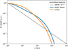 |
Fig. 10 Toy model for the spectra of particles accelerated at sheet base and cone shocks for cluster I. The maximum cut-off energy is close to 500 TeV. (For further description, see the text.) |
5.5 Particle transport
In Sect. 4.4, we inferred a diffusivity of D = (Δx)2/(2s) ~ 0.5–2 pc for streamlines of the magnetic field, where Δx is the linear spatial displacement and s the length along the streamline. Non-thermal particles, to lowest order, follow the large-scale field, performing helical motion. In the transonic sheets, the field shows a quasi-radial morphology (see Fig. 5). This may lead to fast escape of particles if the scattering rate is low. Since constraining turbulence on particle gyro-scales is beyond the capabilities of our approach, this remains an unknown. The cones show a more diverse magnetic field morphology, which includes regions where the fieldlines appear highly tangled, sections of quasi-perpendicular fieldlines in the cluster WTS downstream where the field is amplified, and loops extending outward on various scales. Around the shock, B shows a wide range of obliquities (see Fig. 9, right-most panel). While perpendicular fields in the shock downstream can in principle confine particles close to the shock, it seems likely that any such effect is minor, since particles could still escape through the transonic sheets.
As expected in ideal MHD, fieldlines are anchored in the core from which the originate. This leads to quasi-perpendicular fields at the contact discontinuity at the edge of the superbubble, which could effectively confine particles inside the superbubble. In realistic scenarios, the shell is likely to at least partly break apart due to instabilities (e.g. El-Badry et al. 2019; Lancaster et al. 2024). However, this phenomenon is not well constrained, among other factors because the magnetic field can stabilise the shell (see Chandrasekhar 1961). Our simulations are tailored to studying the cluster core and wind and do not have sufficient resolution at the shell to draw meaningful conclusions.
6 Conclusion
We have performed 3D ideal MHD simulations of stellar winds around compact young massive star clusters. Prominent examples of such objects include Westerlund 1, 30 Doradus C, and R136. We modelled 46 individual stars with M > 40 M⊙ and injected winds kinetically in order to study the 3D flow and magnetic field geometry on the superbubble scale. We included the effects of WR winds, studied clusters with two different radii (Rc = 0.6 pc and 1 pc), and discussed three different scenarios for the magnetic field. Our main conclusions are as follows:
The flow shows an intricate morphology, which significantly deviates from spherical symmetry. We recovered the subsonic cluster core, supersonic collective cluster wind, and tenuous superbubble interior medium expected from 1D theory. The position and power of individual stars critically influences the morphology of the flow. The cluster wind has non-uniform properties and is locally impacted by downstream material from individual stellar winds. For example, regions in the flow path of magnetic stars have an above-average magnetic field;
In addition to the three zones mentioned above, we find that strong stellar winds can extend from the core all the way to the cluster WTS (‘coupled winds’). Secondly, we find transonic sheets extend well beyond the cluster WTS with an internal structure that resembles that of the ‘shock diamond’ phenomenon;
The cluster WTS has a Mach number of MS ~ 10 at the end of the simulation (390 kyr) for a cluster radius of 0.6 pc and MS ~ 6 for 1 pc. Since the typical age of young compact clusters exceeds the simulation time, we conclude that compact clusters (Rc < 2–3 pc) can in general be expected to have a strong cluster WTS. The cluster WTS is found to be non-spherical and smaller in volume compared to 1D theory. The cluster WTS can be sub-divided into regions of quasi-parallel flow and highly oblique flow (‘sheet bases’ and ‘cones’, respectively);
The magnetic field morphology is characterised by loops of various sizes, which stay anchored in the cluster core, as well as coherent quasi-radial field-line bundles extending outward preferentially inside transonic sheets. In the core, the magnetic field is highly tangled and locally dominated by Parker spiral fields from individual stars. The obliquity of the magnetic field varies over the cluster WTS surface. Mixing of flow from magnetic stars into the bulk medium contributes significantly to the observed magnetisation of the bulk flow. Across all runs, we found a median magnetic field magnitude, B, of 8–35 μG in the core and 4–20 μG in the superbubble. Values of up to ~1 mG are reached in the vicinity of magnetic stars. These findings are consistent with previous work simulating only the cluster core (Badmaev et al. 2022). The magnetic field is found to scale slightly steeper that r−1 in the cluster wind;
We discussed particle acceleration and propagation around young compact star clusters. We found a large spread in B in the cluster WTS upstream, which ultimately leads to the prediction of steep particle spectra in the teraelectronvolt energy range (∝E−3 with curvature). This finding is in line with recent γ-ray observations of young clusters (e.g. LHAASO Collaboration 2025). However, we deem the scenario of petaelectronvolt particle acceleration at the cluster WTS as unlikely because the Hillas limit barely reaches 200 TeV in the most highly magnetised regions. Dynamo effects on scales less than 0.01 pc would have to increase the magnitude of B by a factor of at least five over that observed in the simulation to reach petaelectronvolt energies. Streaming instabilities can in principle amplify the magnetic field above the large-scale value from the simulation, but whether they reach saturation on the relevant scales is uncertain.
Our work showcases the non-trivial nature of stellar-wind interaction around young star clusters. Several parameters, such as the distribution and median of B at the cluster WTS, depend on the spatial distribution of stars. Considering that the population of young star clusters detected in γ-rays is highly heterogeneous in terms of age, compactness, ambient medium, and stellar population, developing a unified model of particle acceleration for these regions appears challenging. Physical models of γ-ray emission require an understanding of the stellar population and its history and feedback onto the environment. Nevertheless, the average properties discussed in this work can serve a purpose for order of magnitude estimates and give a qualitative impression of the nature of collective effects. A multi-wavelength effort is required to gain further insight into stellar-wind interaction and magnetic fields in star-cluster environments. Future γ-ray observations with the Large High Altitude Air Shower Observatory (LHAASO) and the Cherenkov Telescope Array Observatory (CTAO) will further characterise the cosmic ray populations in the vicinity of young star clusters and provide valuable constraints for acceleration models. X-ray and radio data can constrain the magnetic field to investigate the plausibility of acceleration to high energies. Infrared studies, particularly at high resolution as facilitated by the James Webb Space Telescope (JWST), can illuminate ambient gas and dust structures, thus constraining the nature of feedback processes.
Acknowledgements
The simulations were carried out at the Max-Planck Computing and Data Facility (MPCDF). We thank the developers of PLUTO and the analysis tool pyPLUTO (Mattia et al. 2025), which have facilitated this work. We acknowledge insightful discussion with A. C. Sander, J. S. Wang, and G. Mattia and are grateful for the constructive feedback from the referee. We thank the organisers and attendees of the TOSCA meeting in autumn 20242 for interdisciplinary discussion.
Appendix A Comparison to 1D theory
This section compares the simulation results to 1D theory (Weaver et al. 1977). Figure A.1 shows the density as a function of radius in the first 100 kyr of the simulation. The familiar bubble structure for a compact cluster is recovered: a decrease in the density in the free wind is followed by an increase behind the cluster WTS, which in turn is followed by a zone of constant density in the superbubble interior. Then, the density rises sharply and beyond the ambient value at the shell. While the prediction by Weaver et al. (1977) for the bubble radius agrees with the position of the shell, the termination shock radius is overestimated, due to multi-dimensional effects (see Sect. 3). Figure A.2 shows the thermal, kinetic, and total energy in the simulation domain for all runs, relative to the injected wind power. This agrees with the Weaver et al. (1977) which predicts that, when cooling is neglected, ~22% of the injected energy goes into kinetic energy and ~78% into thermal energy. Figure A.3 shows density slices of the full simulation domain at 390 kyr, highlighting that the position of the forward shock is consistent with 1D theory over the full simulation run time.
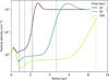 |
Fig. A.1 Radial density profile of the simulated superbubble for cluster I in the initial 100 kyr of the simulation. The dashed and dotted lines indicate the cluster-wind termination shock and bubble radii according to the spherically symmetric, analytic model by Weaver et al. (1977). |
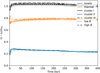 |
Fig. A.2 Kinetic and thermal energy in the full simulation domain relative to the total injected energy, ϵinj = Lwt, for different simulations. The initial energy, ϵ0, is subtracted. Magnetic energy is not shown but is below the percent level. |
 |
Fig. A.3 Density slices of cluster I (top) and III (bottom) showing the full simulation domain at 390 kyr. Black circles indicate the superbubble radius predicted by Weaver et al. (1977). |
Appendix B Star clusters
In Table B.1 we provide the stellar content of our model cluster. For a discussion on how the parameters where selected (see Sect. 2). Figure B.1 shows 3D renderings of cluster I, II, and III.
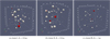 |
Fig. B.1 Three-dimensional renderings of the three different model clusters analysed in this work. All clusters have the same stellar content listed in Table B.1. The size of the sphere is scaled by wind power. Magnetic stars are marked in red. The lines indicate the orientation of the magnetic axes. Clusters I and II have the same compactness Rc = 0.6 pc and only differ in the spatial distribution of stars. Most notably, a rather powerful magnetic star is located close to the centre in cluster II, while in cluster I, it is at the outskirts. Cluster III is less compact, Rc = 1 pc. |
Parameters of the stars in our model cluster. Shown are stellar mass, M; effective temperature, Teff; radius, R; main-sequence lifetime, tMS; mass-loss rate, ![Mathematical equation: $\[\dot{M}\]$](/articles/aa/full_html/2025/06/aa54057-25/aa54057-25-eq29.png) ; terminal wind velocity, u∞; and wind power,
; terminal wind velocity, u∞; and wind power, ![Mathematical equation: $\[L_{\mathrm{w}}=0.5 \dot{M} u_{\infty}^{2}\]$](/articles/aa/full_html/2025/06/aa54057-25/aa54057-25-eq30.png) .
.
Appendix C Supplementary plots on the magnetic field
Figure C.1 shows the upstream distributions of B for different simulation runs. We note that cluster II shows significantly fewer high B outliers than cluster I, which is discussed in the main text. This is due to the more central location of the magnetic star in the star cluster for cluster II. Figures C.2–C.5 show radial profiles of the mean magnitude of B for the simulation runs not included in the main text. The same general trends can be observed across all profiles. We note, however, the small extension of the cluster wind (20 > MS > 3) for the cluster with Rc = 1 pc instead of 0.6 pc (cluster III, Fig. C.3) at 200 kyr. This demonstrates that the cluster wind requires a longer time to reach a given Mach number for less compact clusters. Even at 390 kyr, the transonic component of the cluster wind (3 > MS > 1) is > 10% for most radii.
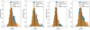 |
Fig. C.1 Distribution of magnetic field magnitude in the immediate cluster-wind termination shock upstream clusters III, II, the low B cluster, and the high B cluster (from left to right). We note that cluster II shows fewer high B outliers than cluster I (see Fig. 9 in the main text). Both clusters differ only differ in the spatial distribution of stars (see Fig. B.1). For further context, we refer to Sect. 5.2. |
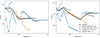 |
Fig. C.2 Radial profiles of the mean magnitude of B for cluster I in different regions. The left panel shows radial profiles at 200 kyr and the right at 390 kyr. (For further context, see Sect. 4.3.) |
References
- Amato, E., & Blasi, P. 2006, MNRAS, 371, 1251 [NASA ADS] [CrossRef] [Google Scholar]
- Axford, W. I., Leer, E., & Skadron, G. 1977, in International Cosmic Ray Conference, 11, International Cosmic Ray Conference, 132 [Google Scholar]
- Badmaev, D. V., Bykov, A. M., & Kalyashova, M. E. 2022, MNRAS, 517, 2818 [NASA ADS] [CrossRef] [Google Scholar]
- Badmaev, D. V., Bykov, A. M., & Kalyashova, M. E. 2024, MNRAS, 527, 3749 [Google Scholar]
- Balsara, D. S., & Spicer, D. 1999, J. Computat. Phys., 148, 133 [Google Scholar]
- Bell, A. R. 1978, MNRAS, 182, 147 [Google Scholar]
- Bell, A. R. 2004, MNRAS, 353, 550 [Google Scholar]
- Bell, A. R. 2005, MNRAS, 358, 181 [NASA ADS] [CrossRef] [Google Scholar]
- Bell, A. R., & Lucek, S. G. 2001, MNRAS, 321, 433 [CrossRef] [Google Scholar]
- Bell, A. R., Schure, K. M., & Reville, B. 2011, MNRAS, 418, 1208 [CrossRef] [Google Scholar]
- Blandford, R. D., & Ostriker, J. P. 1978, ApJ, 221, L29 [Google Scholar]
- Bykov, A. M., & Fleishman, G. D. 1992, MNRAS, 255, 269 [NASA ADS] [CrossRef] [Google Scholar]
- Cantó, J., Raga, A. C., & Rodríguez, L. F. 2000, ApJ, 536, 896 [CrossRef] [Google Scholar]
- Chandrasekhar, S. 1961, Hydrodynamic and Hydromagnetic Stability, In International Series of Monographs on Physics (Oxford: Clarendon) [Google Scholar]
- Chevalier, R. A., & Clegg, A. W. 1985, Nature, 317, 44 [Google Scholar]
- Chu, Y.-H. 2008, in IAU Symposium, 250 (Proceedings of the International Astronomical Union), 341 [Google Scholar]
- Dyson, J. E., & de Vries, J. 1972, A&A, 20, 223 [NASA ADS] [Google Scholar]
- Eker, Z., Bakış, V., Bilir, S., et al. 2018, MNRAS, 479, 5491 [NASA ADS] [CrossRef] [Google Scholar]
- Ekström, S., Georgy, C., Eggenberger, P., et al. 2012, A&A, 537, A146 [Google Scholar]
- El-Badry, K., Ostriker, E. C., Kim, C.-G., Quataert, E., & Weisz, D. R. 2019, MNRAS, 490, 1961 [CrossRef] [Google Scholar]
- Ferrand, G., & Marcowith, A. 2010, A&A, 510, A101 [NASA ADS] [CrossRef] [EDP Sciences] [Google Scholar]
- Gabici, S., Evoli, C., Gaggero, D., et al. 2019, Int. J. Mod. Phys. D, 28, 1930022 [CrossRef] [Google Scholar]
- Grunhut, J. H., Wade, G. A., Neiner, C., et al. 2017, MNRAS, 465, 2432 [NASA ADS] [CrossRef] [Google Scholar]
- Gupta, S., Nath, B. B., & Sharma, P. 2018, MNRAS, 479, 5220 [NASA ADS] [CrossRef] [Google Scholar]
- Gupta, S., Nath, B. B., Sharma, P., & Eichler, D. 2020, MNRAS, 493, 3159 [CrossRef] [Google Scholar]
- Hamann, W. R., Gräfener, G., Liermann, A., et al. 2019, A&A, 625, A57 [NASA ADS] [CrossRef] [EDP Sciences] [Google Scholar]
- HESS Collaboration (Abramowski, A., et al.) 2011, A&A, 525, A46 [NASA ADS] [CrossRef] [EDP Sciences] [Google Scholar]
- HESS Collaboration (Aharonian, F., et al.) 2022, A&A, 666, A124 [NASA ADS] [CrossRef] [EDP Sciences] [Google Scholar]
- HESS Collaboration (Aharonian, F., et al.) 2024, ApJ, 970, L21 [Google Scholar]
- Higdon, J. C., & Lingenfelter, R. E. 2005, ApJ, 628, 738 [Google Scholar]
- Hillas, A. M. 1984, ARA&A, 22, 425 [Google Scholar]
- Klepach, E. G., Ptuskin, V. S., & Zirakashvili, V. N. 2000, Astropart. Phys., 13, 161 [NASA ADS] [CrossRef] [Google Scholar]
- Krause, M., Fierlinger, K., Diehl, R., et al. 2013, A&A, 550, A49 [NASA ADS] [CrossRef] [EDP Sciences] [Google Scholar]
- Kroupa, P. 2002, Science, 295, 82 [Google Scholar]
- Krymskii, G. F. 1977, Akad. Nauk SSSR Dokl., 234, 1306 [Google Scholar]
- Kumar, N., & Reville, B. 2021, ApJ, 921, L14 [Google Scholar]
- Lagage, P. O., & Cesarsky, C. J. 1983, A&A, 125, 249 [NASA ADS] [Google Scholar]
- Lancaster, L., Ostriker, E. C., Kim, J.-G., & Kim, C.-G. 2021, ApJ, 914, 90 [NASA ADS] [CrossRef] [Google Scholar]
- Lancaster, L., Ostriker, E. C., Kim, C.-G., Kim, J.-G., & Bryan, G. L. 2024, ApJ, 970, 18 [Google Scholar]
- Lee, J. C., Sandstrom, K. M., Leroy, A. K., et al. 2023, ApJ, 944, L17 [NASA ADS] [CrossRef] [Google Scholar]
- LHAASO Collaboration 2024, Sci. Bull., 69, 449 [NASA ADS] [CrossRef] [Google Scholar]
- LHAASO Collaboration 2025, Sci. China Phys. Mech. Astron., 68, 279502 [Google Scholar]
- Mackey, J., Mathew, A., Ali, A. A., et al. 2025, A&A, 696, A91 [NASA ADS] [CrossRef] [EDP Sciences] [Google Scholar]
- Martins, F., Schaerer, D., & Hillier, D. J. 2005, A&A, 436, 1049 [NASA ADS] [CrossRef] [EDP Sciences] [Google Scholar]
- Matthews, J. H., Bell, A. R., Blundell, K. M., & Araudo, A. T. 2017, MNRAS, 469, 1849 [Google Scholar]
- Mattia, G., Crocco, D., Fuksman, D. M., et al. 2025, arXiv e-prints [arXiv:2501.09748v1] [Google Scholar]
- Mignone, A., Bodo, G., Massaglia, S., et al. 2007, ApJS, 170, 228 [Google Scholar]
- Mizuno, Y., Gómez, J. L., Nishikawa, K.-I., et al. 2015, ApJ, 809, 38 [Google Scholar]
- Morlino, G., Blasi, P., Peretti, E., & Cristofari, P. 2021, MNRAS, 504, 6096 [NASA ADS] [CrossRef] [Google Scholar]
- Parker, E. N. 1958, ApJ, 128, 664 [Google Scholar]
- Portegies Zwart, S. F., McMillan, S. L., & Gieles, M. 2010, ARA&A, 48, 431 [NASA ADS] [CrossRef] [Google Scholar]
- Reville, B., Giacinti, G., & Scott, R. 2021, MNRAS, 502, 4137 [NASA ADS] [CrossRef] [Google Scholar]
- Rogers, H., & Pittard, J. M. 2013, MNRAS, 431, 1337 [CrossRef] [Google Scholar]
- Sander, A. A. C., Hamann, W. R., Todt, H., et al. 2019, A&A, 621, A92 [NASA ADS] [CrossRef] [EDP Sciences] [Google Scholar]
- Schaller, G., Schaerer, D., Meynet, G., & Maeder, A. 1992, A&AS, 96, 269 [Google Scholar]
- Schinnerer, E., & Leroy, A. K. 2024, ARA&A, 62, 369 [NASA ADS] [CrossRef] [Google Scholar]
- Seo, J., Kang, H., & Ryu, D. 2018, J. Korean Astron. Soc., 51, 37 [NASA ADS] [Google Scholar]
- Townsley, L. K., Broos, P. S., Feigelson, E. D., et al. 2006, AJ, 131, 2140 [Google Scholar]
- Unger, M., & Farrar, G. R. 2024, ApJ, 970, 95 [NASA ADS] [CrossRef] [Google Scholar]
- Vieu, T., & Reville, B. 2023, MNRAS, 519, 136 [Google Scholar]
- Vieu, T., Gabici, S., Tatischeff, V., & Ravikularaman, S. 2022, MNRAS, 512, 1275 [NASA ADS] [CrossRef] [Google Scholar]
- Vieu, T., Härer, L., & Reville, B. 2024a, MNRAS, 530, 4747 [Google Scholar]
- Vieu, T., Larkin, C. J. K., Härer, L., et al. 2024b, MNRAS, 532, 2174 [NASA ADS] [CrossRef] [Google Scholar]
- Vink, J. S., de Koter, A., & Lamers, H. J. G. L. M. 2001, A&A, 369, 574 [NASA ADS] [CrossRef] [EDP Sciences] [Google Scholar]
- Weaver, R., McCray, R., Castor, J., Shapiro, P., & Moore, R. 1977, ApJ, 218, 377 [Google Scholar]
- Wentzel, D. G. 1974, ARA&A, 12, 71 [NASA ADS] [CrossRef] [Google Scholar]
- Xu, R., Spitkovsky, A., & Caprioli, D. 2020, ApJ, 897, L41 [NASA ADS] [CrossRef] [Google Scholar]
- Zakhozhay, V. A. 2013, Kinemat. Phys. Celest. Bodies, 29, 195 [Google Scholar]
All Tables
Parameters of the stars in our model cluster. Shown are stellar mass, M; effective temperature, Teff; radius, R; main-sequence lifetime, tMS; mass-loss rate, ; terminal wind velocity, u∞; and wind power, .
All Figures
|
Fig. 1 Density slices for cluster I (Rc = 0.6 pc, top) and cluster III (Rc = 1 pc, bottom). The inner ±8 pc are shown, which excludes the superbubble shell. In the left-most panels (a and e), all stars are on the main sequence. The cluster wind is in a quasi-stationary state, slowly expanding over time but not changing geometry. At t > 200 kyr (panels b–d and f–h), the most massive stars consecutively evolve into WR stars. The flow rearranges into a new quasi-stationary state within ~20 kyr after each new WR wind (see panels b–c and e–f). The wind termination shock has a complex, non-spherical geometry, which appears different in different slices (see panels g–h). The white circle in panels g–h indicates the shock radius predicted by 1D analytical theory (Weaver et al. 1977). |
| In the text | |
|
Fig. 2 Slices highlighting the properties of shocks in and around the star cluster. (a) Individual stellar winds reach Mach numbers of MS ~ 100 and the cluster wind has MS ~ 10. The transonic sheets, which are found downstream of the cluster-wind termination shock, have MS ~ 1–2. (b) The flow is highly super-Alfvénic, except in a small number of localised regions in the superbubble and cluster core. (c) The cluster-wind termination shock is compressive across its entire surface, as shown by the negative divergence of the velocity field. Alternating compression and rarefaction zones inside the transonic sheets indicate a structure similar to that seen in the ‘shock diamond’ phenomenon. The values have been normalised to the maximum. Panels a and b show a z-axis slice of cluster I at 330 kyr. Panel c shows the same slice at 200 kyr. |
| In the text | |
|
Fig. 3 Surfaces of constant sonic Mach number visualising (a) the cluster-wind termination shock and (b) transonic sheets. The two panels in (a) show the orientation of the magnetic field, B (left), and the flow velocity, u (right), with respect to the Mach surface normal, n. In the latter plot, cones (blue, dominated by perpendicular flow) can be clearly distinguished from sheet base shocks (red, inbetween adjacent cones) and coupled stellar winds (red, in the centre of cones). In panel b, the MS = 1 surface is over-plotted onto the MS = 3 surface surface in transparent white, highlighting that sheets extend outward from regions of parallel flow. The panels show cluster I at 390 kyr. |
| In the text | |
|
Fig. 4 Slices of magnetic field magnitude highlighting the non-uniformity of the field. The non-uniformity can partly be attributed to the five magnetic stars in the cluster. The magnetic field reaches 1 mG in the cluster core and can fall to values of 0.1 μG in the cluster wind. Large asymmetries persist into the superbubble, although they smooth out slowly over time. Two main observations are (1) field amplification behind the wind termination shock (e.g. right-most panel) and (2) mixing of flow from magnetic stars into the bulk medium (e.g. left-most panel). The figure shows data for cluster III sliced along the z-axis. |
| In the text | |
|
Fig. 5 Streamlines of the magnetic field coloured by magnitude. In the upper panel, streamline seed points are placed within the radius of the star cluster. This highlights the tangled morphology arising from the interaction of Parker spiral stellar magnetic fields. The lower panel shows streamlines for a seed point radius comparable to the size of the cluster-wind termination shock (5 pc) over-plotted onto the surface where the sonic Mach number equals three. The surface colour shows the orientation of the flow velocity, u, with respect to the surface normal, n. We note the quasi-radial streamline bundles, which are dragged outward by coherent flows. Such flows are present, for example, in transonic sheets (see Fig. 3b). The figure shows cluster I at 390 kyr. |
| In the text | |
|
Fig. 6 Magnetic field in the cluster core (left) and superbubble interior (right). Triangles mark distributions before the WR onset at 200 kyr, and circles indicate distributions after the WR onset at 390 kyr. Colours indicate different simulation runs (see Table 1 for run parameters). Filled markers show the mean, empty markers the median. Whiskers indicate the 25th and 75th percentiles. Asymmetries due to local wind interactions are larger in the core, as evident by the broader distributions, but are reduced when the flow reaches the superbubble. We note that the distributions are shown in log space. |
| In the text | |
|
Fig. 7 Radial profiles of the mean magnitude of the magnetic field, ⟨B⟩, in different regions for cluster II. The upper panel shows the profiles at 200 kyr, and the lower panels shows them at 390 kyr. The profiles were obtained by averaging over 10 000 randomly drawn line-outs. Points are only plotted where at least 10% of line-outs pass through the indicated region. ⟨B⟩ scales approximately as r−1 in the supersonic cluster wind. The hump in the stellar winds profile close to 0.6 pc stems from magnetic stars and is traced by a hump in the subsonic core medium. This indicates that wind material from magnetic stars significantly increases the magnetisation of the bulk. |
| In the text | |
|
Fig. 8 Streamline diffusivity for seed points placed within spheres of the indicated radii at 200 kyr (left) and 390 kyr (right). Triangles, circles, and squares indicate clusters I, II, and III, respectively. The near linear increase for the 5 pc seed cloud radius is due to quasi-radial field-line bundles embedded in transonic sheets (cf. Fig. 5, lower panel) and the levelling-off is due to fieldlines travelling close to the superbubble edge looping back to the core. The variation between clusters I and II, which only differ in the spatial distribution of stars, illustrates the importance of local wind interactions. |
| In the text | |
|
Fig. 9 Properties in the immediate upstream of sheet base shocks and wind cones at 390 kyr of simulation time. The histograms were compiled from values along 10 000 randomly drawn line-outs. The distribution of values at sheet bases and cones is similar for most parameters, except the velocity across the shock, u · n (panel 3). (For further description, see the text.) |
| In the text | |
|
Fig. 10 Toy model for the spectra of particles accelerated at sheet base and cone shocks for cluster I. The maximum cut-off energy is close to 500 TeV. (For further description, see the text.) |
| In the text | |
|
Fig. A.1 Radial density profile of the simulated superbubble for cluster I in the initial 100 kyr of the simulation. The dashed and dotted lines indicate the cluster-wind termination shock and bubble radii according to the spherically symmetric, analytic model by Weaver et al. (1977). |
| In the text | |
|
Fig. A.2 Kinetic and thermal energy in the full simulation domain relative to the total injected energy, ϵinj = Lwt, for different simulations. The initial energy, ϵ0, is subtracted. Magnetic energy is not shown but is below the percent level. |
| In the text | |
|
Fig. A.3 Density slices of cluster I (top) and III (bottom) showing the full simulation domain at 390 kyr. Black circles indicate the superbubble radius predicted by Weaver et al. (1977). |
| In the text | |
|
Fig. B.1 Three-dimensional renderings of the three different model clusters analysed in this work. All clusters have the same stellar content listed in Table B.1. The size of the sphere is scaled by wind power. Magnetic stars are marked in red. The lines indicate the orientation of the magnetic axes. Clusters I and II have the same compactness Rc = 0.6 pc and only differ in the spatial distribution of stars. Most notably, a rather powerful magnetic star is located close to the centre in cluster II, while in cluster I, it is at the outskirts. Cluster III is less compact, Rc = 1 pc. |
| In the text | |
|
Fig. C.1 Distribution of magnetic field magnitude in the immediate cluster-wind termination shock upstream clusters III, II, the low B cluster, and the high B cluster (from left to right). We note that cluster II shows fewer high B outliers than cluster I (see Fig. 9 in the main text). Both clusters differ only differ in the spatial distribution of stars (see Fig. B.1). For further context, we refer to Sect. 5.2. |
| In the text | |
|
Fig. C.2 Radial profiles of the mean magnitude of B for cluster I in different regions. The left panel shows radial profiles at 200 kyr and the right at 390 kyr. (For further context, see Sect. 4.3.) |
| In the text | |
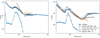 |
Fig. C.3 Same as Fig. C.2 but for cluster III. |
| In the text | |
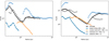 |
Fig. C.4 Same as Fig. C.2 but for the low B cluster. |
| In the text | |
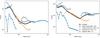 |
Fig. C.5 Same as Fig. C.2 but for the high B cluster. |
| In the text | |
Current usage metrics show cumulative count of Article Views (full-text article views including HTML views, PDF and ePub downloads, according to the available data) and Abstracts Views on Vision4Press platform.
Data correspond to usage on the plateform after 2015. The current usage metrics is available 48-96 hours after online publication and is updated daily on week days.
Initial download of the metrics may take a while.