| Issue |
A&A
Volume 698, June 2025
|
|
|---|---|---|
| Article Number | A100 | |
| Number of page(s) | 12 | |
| Section | Stellar structure and evolution | |
| DOI | https://doi.org/10.1051/0004-6361/202554051 | |
| Published online | 03 June 2025 | |
Dissimilar magnetically driven accretion on the components of V4046 Sagittarii
Department of Astronomy, University of Geneva, Chemin Pegasi 51, CH-1290 Versoix, Switzerland
⋆ Corresponding author: This email address is being protected from spambots. You need JavaScript enabled to view it.
Received:
6
February
2025
Accepted:
8
April
2025
Abstract
Context. The accretion of pre-main sequence (PMS) stars is a key process in stellar formation that governs mass assembly, influences angular momentum conservation and stellar internal structure, and shapes disc evolution, which serves as the birthplace of exoplanets. Classical T Tauri stars (cTTSs), low-mass PMS stars actively accreting from a disc, hold a well-described magnetospheric accretion model. Their strong, inclined dipole magnetic fields truncate the disc at a few stellar radii, channelling material along magnetic field lines to fall onto the stellar surface near the dipole pole. However, this paradigm assumes the presence of a single star, and a complete description of the accretion process in multiple systems remains to be achieved.
Aims. Building on our previous work on DQ Tau and AK Sco, our aim is to describe the accretion processes in cTTS binaries, accounting for the influence of stellar magnetic fields. Specifically, we explored how the magnetospheric accretion model of cTTSs can be applied to V4046 Sgr, a spectroscopic binary composed of equal-mass and coeval cTTSs in a circular orbit with synchronous rotation, surrounded by a circumbinary disc.
Methods. We analysed a time series of ESPaDOnS spectra covering several orbital cycles. A variability analysis was performed on the radial velocities and on the Balmer, He i D3, and Ca ii emission lines, which are associated with the accretion process.
Results. We identified the secondary as the system's main accretor, operating in an unstable regime. Additionally, we detected an accretion funnel flow connecting the dipole pole of the primary star with a nearby bulk of gas.
Conclusions. We concluded that the two components exhibit dissimilar accretion patterns. The primary operates in an ‘ordered chaotic’ regime, where accretion funnel flows and accretion tongues (which penetrate the magnetosphere to reach the stellar equator) coexist. Conversely, the secondary appears to be in a chaotic regime, where the accretion tongues dominate.
Key words: accretion, accretion disks / techniques: spectroscopic / stars: individual: V4046 Sgr / stars: variables: T Tauri, Herbig Ae/Be
© The Authors 2025
 Open Access article, published by EDP Sciences, under the terms of the Creative Commons Attribution License (https://creativecommons.org/licenses/by/4.0), which permits unrestricted use, distribution, and reproduction in any medium, provided the original work is properly cited.
This article is published in open access under the Subscribe to Open model. This email address is being protected from spambots. You need JavaScript enabled to view it. to support open access publication.
1. Introduction
The accretion process in classical T Tauri stars (cTTSs), which are young low-mass stellar objects still surrounded by a disc from which they accrete material, is commonly described by the magnetospheric accretion model (Hartmann et al. 1994). In this model, the strong dipolar magnetic field of such systems exerts magnetic pressure on the disc at the magnetospheric radius, forcing material to leave the disc plane and fall onto the stellar surface along magnetic field lines. While simulations have successfully reproduced this framework (see the review by Romanova & Owocki 2015), and its characteristics are often observed in cTTSs, a major assumption underlying the model is that the system must be single. Given that most low-mass stars form in multiple systems (Offner et al. 2023), this accretion model only applies to a minority of stars. Therefore, dedicated studies are required to develop a framework that can accommodate multiple systems. This work extends previous efforts in this direction, such as studies of the eccentric cTTS binaries DQ Tau and AK Sco Pouilly et al. (2023, 2024a), by investigating systems with different orbital configurations, starting with the present study on V4046 Sagittarii.
V4046 Sgr is a type II spectral binary (SB2) system (possibly part of a hierarchical quadruple system, with the binary GSC0739 as a distant–∼12 350 au–companion; Kastner et al. 2011) comprising two cTTSs of spectral types K5 and K7. The system is surrounded by a circumbinary disc with an inner radius of 0.35 au. The two stars orbit in a circularised configuration with a projected separation of approximately 2.5 R⊙. Their rotational periods are synchronised with the 2.42-day orbital period, and the rotation axes are aligned with both the orbital motion and the disc, which is observed at an inclination of 35°. The disc's mass is estimated to be between 0.01 and 0.08 M⊙, with its thickness increasing to 0.2 au at the outer edge, located approximately 100 au from the system's centre (Quast et al. 2000).
Further characterisation of the large-scale circumbinary disc's structure was provided by Martinez-Brunner et al. (2022), who used ALMA 1.3 mm continuum imaging, SPHERE-IRDIS polarised images, and a well-sampled spectral energy distribution. Their model predicts the presence of an inner disc at 5 au, but it is too faint to be detected by ALMA. Nevertheless, they detected a narrow ring at 13 au with a width of 2.46 au and a height ten times lower, a 10 au gap, and another ring at 24 au. This second ring exhibits peak intensity at 30 au and a break in luminosity at 36 au.
The orbital parameters of V4046 Sgr were refined by Stempels & Gahm (2004) through a series of UVES spectra. Their analysis yielded a more consistent mass ratio for the components, confirmed the circularisation of the orbit, and verified the synchronous rotation. Notably, they determined an orbital period of 2.4213459 days, with semi-amplitudes K1=54.16 km s−1 and K2=56.61 km s−1. A spectral line analysis revealed low levels of veiling (∼5% of the continuum at 620 nm) and minimal or absent extinction. An examination of the emission lines indicated a Ca ii K line with a narrow component (NC) for both stars, closely tied to the binary orbit, suggesting formation in extended chromospheres around each star. Additionally, they decomposed higher-order Balmer lines (H8, H9, H10), which shared similar shapes, into four components: an NC (close to the Ca ii K NC) and a broad component (BC) for both stars. The BC varied with the orbital period, showing an amplitude of 80 km s−1, larger than the stellar orbital amplitude. They concluded that these BC emissions originate from gas bulks co-rotating at 6.9 R⊙ from the centre of mass, corresponding to approximately 1.15 R★ from each star. This is well within the inner edge of the circumbinary disc and near the co-linear Lagrange points. The stars appear to accrete from these bulks, with the BC's variable equivalent width (EW) indicating variable accretion rates.
In 2009, V4046 Sgr was the subject of a multi-instrument campaign that included X-ray observations with XMM-Newton (Argiroffi et al. 2012). These observations revealed the periodic signature of an accretion shock at half the orbital period. Three hypotheses were proposed to explain this signal: (i) one component has two accretion shock regions at opposite longitudes; (ii) one component has a single accretion region that emits maximally when the shock is viewed edge-on; (iii) both components have symmetric shocks located 180° apart relative to the binary rotation axis.
The campaign also included quasi-simultaneous optical observations with the Echelle SpectroPolarimetric Device for Observation of Stars (ESPaDOnS; Donati 2003) mounted on the Canada-France-Hawaii Telescope (CFHT). Donati et al. (2011) analysed these data to study the system's large-scale magnetic field. The magnetic topologies of the two components were found to be complex and weak, reflecting the partly convective internal structure of these 12 Myr old stars. The primary exhibited a mean field strength (〈B〉=230 G) with a dominant azimuthal component and a maximum field strength (Bmax) of 500 G in an arc-like structure near the pole. Its dipole component was weak (Bdip = 100 G), non-axisymmetric, and had an obliquity of 60°, facing the observer at phase 0.8. The secondary had a weaker mean field strength (Bmax = 170 G) and a highly oblique dipole (Bdip = 70 G, obliquity 90°), facing the observer at phase 0.1. Surface maps revealed cool spots near the rotational poles of both stars, slightly offset towards the hemispheres facing their companion. The low-contrast extended Ca II infrared triplet (IRT) excess emissions suggested that accretion occurs at multiple sites on the stellar surface, rather than being concentrated in a specific region.
Hahlin & Kochukhov (2022) also used the ESPaDOnS dataset to study the small-scale magnetic field through Zeeman intensification of a Ti multiplet. They found similar small-scale field strengths for both components (1.96 and 1.83 kG for the primary and secondary, respectively) and nearly identical filling factors. Their analysis yielded a lower luminosity ratio (LR = 1.27) than that determined by Stempels & Gahm (2004) and higher vsini values (15.1 and 14.4 km s−1) for the primary and secondary, respectively.
In this paper we provide a detailed description of the system's accretion process using the same dataset employed for magnetic field studies. The observations are described in Sect. 2, the analyses and results are presented in Sect. 3, and these findings are discussed in Sect. 4. We conclude this work in Sect. 5.
2. Observations
The dataset used in this work is the same as that utilised by Donati et al. (2011) and Hahlin & Kochukhov (2022) for their magnetic analysis of V4046 Sgr. It consists of eight spectropolarimetric observations acquired at the CFHT using ESPaDOnS.
This instrument covers a wavelength range of 370−1050 nm, achieving a resolving power of 68 000. It was operated in spectropolarimetric mode, meaning that each observation consists of four sub-exposures taken with different polarimeter configurations. The observations were reduced using the automatic pipeline Libre-ESpRIT, which combines the sub-exposures to optimise the extraction of the ESPaDOnS unpolarised (Stokes I) and circularly polarised (Stokes V) spectra.
For this work, only the Stokes I spectra were used, as the Stokes V spectra were fully analysed in Donati et al. (2011), but we included in Sect. 4 a discussion about the overall Stokes I and V results. The observations were carried out between 3 September 2009 and 9 September 2009, following a one-day cadence (except for 6 September 2009, when the star was observed twice). The values for the signal-to-noise ratio (S/N) per spectral pixel at order 31 (730 nm) range between 140 and 179. A journal of observations is provided in Table 1.
ESPaDOnS observations used in this work.
3. Results
3.1. Least-squares deconvolution profiles and radial velocities
To study the orbital modulation through the radial velocity (Vr) variation, we utilised the least-squares deconvolution (LSD; Donati et al. 1997) Stokes I profiles, which represent a weighted average of as many photospheric lines as possible. These profiles were computed using the LSDpy1 Python package.
The LSD weights were normalised using an intrinsic line depth of 0.2, a mean Landé factor of 1.310, and a mean wavelength of 500 nm. Photospheric lines were selected by creating a mask based on the VALD database line list (Ryabchikova et al. 2015), with MARC (Gustafsson et al. 2008) atmospheric models tailored to the parameters of V4046 Sgr. We then removed emission lines and heavily blended lines using the SpecpolFlow2 Python package, resulting in approximately 15 000 lines used to compute the LSD profiles. The resulting profiles are presented in Fig. 1, with their S/N ranging from 1512 to 2041.
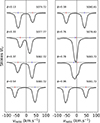 |
Fig. 1. LSD Stokes I profiles of V4046 Sgr. The blue (red) ticks illustrate the velocity of the A (B) component. The orbital phases (computed from Eq. 1) and HJDs (−2 450 000 d) are indicated respectively on the left and right of each profile. |
To derive the Vr, we employed the disentangling procedure described in Pouilly et al. (2023). This method was originally designed to determine a mean disentangled profile for each component based on a time series across the orbital cycle. However, the procedure necessitates a Vr optimisation during the process, enabling us to extract a precise Vr for each component in every observation. The Vr values obtained through this method are presented in Fig. 2 and summarised in Appendix A.
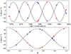 |
Fig. 2. Radial velocity curves of the primary (blue) and secondary (red) components of V4046 Sgr. The top panel represents velocity as function of the HJD, while the bottom panel shows the curve folded in phase using the ephemeris of Eq. (1). The dash-dotted curve shows the orbital solution using the parameters of Table 2. The error bars are included in this plot, but are smaller than the marker sizes. |
Orbital elements derived from the Vr curves.
Finally, we utilised a Levenberg-Marquardt algorithm to simultaneously fit an orbital solution to the individual Vr curves and their difference, allowing us to derive the orbital parameters of the system. The values obtained are summarised in Table 2. The derived orbital period, Porb = 2.42246 ± 0.00055 d, is consistent within 1σ of the value reported by Stempels & Gahm (2004), and within 2σ of Quast et al. (2000). Thus, to define the orbital phases used in this work, we use the ephemeris
 (1)
(1)
where E is the orbital cycle. We note that this ephemeris is slightly different from Donati et al. (2011) (T0 = 2 446 998.335 and Porb = 2.4213459 d), implying small differences in the phases used in this work but yielding conjunctions at phases 0.25 and 0.75, as expected.
3.2. Balmer lines
The accretion funnel flows invoked by the magnetospheric accretion process meet the conditions required for the emission of hydrogen lines such as Hα, Hβ, and Hγ of the Balmer series (Muzerolle et al. 2001). These lines are therefore suitable for studying the accretion process. Figure 3 presents the residual profiles of these three lines.
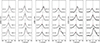 |
Fig. 3. Hα (left two pannels), Hβ (middle two panels), and Hγ (right two panels) residual profiles of V4046 Sgr. These profiles are ordered by orbital phase and corrected from the radial velocity of the primary. The red ticks indicate the velocity of the secondary. The orbital phases and HJDs are indicated respectively on the left and right of each profile. |
To compute these profiles, we used a photospheric template with a temperature similar to that of the V4046 Sgr components: V819 Tau, a non-accreting T Tauri star with vsini = 9.5 km s−1 (Donati et al. 2015). We combined two spectra of V819 Tau, accounting for the luminosity ratio of the V4046 Sgr components (LR = 1.27, Hahlin & Kochukhov 2022), to perform the photospheric correction.
These lines exhibit significant variability and appear to be primarily emitted at the velocity of the secondary component, which may indicate that the secondary is the system's main accretor. In the Hγ line, one can observe the presence of a redshifted absorption at phases 0.33 and 0.37, extending up to +350 km s−1. This behaviour, known as an inverse P Cygni (IPC) profile, indicates infalling material passing through the line of sight, which is characteristic of the magnetospheric accretion process.
We computed the 2D periodograms of the three lines, consisting of a generalised Lomb-Scargle periodogram (GLS) calculated in each velocity channel, enabling us to study the periodic modulations within the lines. In the primary's velocity frame the lines behave similarly, exhibiting a periodic variability of the red wing that is consistent with the orbital period, albeit with a relatively high false alarm probability (FAP = 10−1, computed from the prescription of Baluev 2008). Additionally, a signal over the blue wing appears slightly higher in frequency than, but still consistent with, the orbital period (FAP = 10−2). These two signals are consistent with an orbital modulation induced by the emission from the secondary.
Interestingly, the 2D periodograms also reveal a signal around f = 0.3 d−1 at the centre of the line. While the FAP associated with this period is high for Hα and Hβ (>10−1), it is significantly lower for Hγ (10−2).
In the secondary's velocity frame, only the Hα blue wing exhibits a significant periodicity detection, consistent with the orbital period and with a FAP of 10−1. At the line centre, the signal with the lowest FAP occurs at a frequency of approximately 0.95 d−1, which corresponds to the time series sampling.
To identify the different variabilities within these lines, we focused on Hγ, which exhibits multiple periodicities, to perform a cross-correlation matrix analysis. This tool allows us to identify the correlation between variability regions within a line by calculating a linear correlation coefficient (here, a Pearson coefficient) in each velocity channel of two lines (or twice the same line for an autocorrelation matrix). A correlation (near 1) indicates variability dominated by a single physical process, while an anti-correlation (near −1) may also indicate two correlated processes.
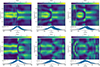 |
Fig. 4. 2D periodograms of Hα (left), Hβ (middle), and Hγ (right) residual lines in the primary's (top row) and secondary's (bottom row) velocity frame. The colour scales the power of the periodogram and the white dotted line highlights the orbital period. The mean profile and it variance are shown at the bottom of each plot in black and blue, respectively. The mirroring effect is due to the one-day aliasing, a spectral leakage of the Fourier transform reproducing, with the real signal, the observation sampling. The signal and its alias are disentangled thanks to the FAP. |
The autocorrelation matrix of Hγ is shown in Fig. 5. When the line is set in the velocity frame of the primary, the correlation matrix exhibits three main correlated regions (with r>0.9). Two of these regions are symmetric around the line centre (between −250 and −50 km s−1, and between +30 and +200 km s−1) and are slightly anti-correlated with each other (r∼−0.7). This behaviour typically traces the motion of the emission from the secondary. The third correlated region lies between +200 and +350 km s−1, a velocity range consistent with the IPC profile observed at phases 0.33 and 0.37.
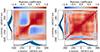 |
Fig. 5. Hγ residual line autocorrelation matrix in the velocity frame of the primary (left) and secondary (right). The colour-code scales the correlation coefficient: red represents a strong correlation and blue shows a strong anti-correlation. The plots along the x- and y-axes represent the corresponding mean line profile (black) and its variance (blue). |
When the line is set in the velocity frame of the secondary, the autocorrelation matrix appears entirely different, as expected if the emission from the secondary differs from that of the primary. The three correlated regions are now located between −150 and 0 km s−1, 0 and +80 km s−1, and +120 and +230 km s−1.
Finally, we examined the EW variation. The three lines exhibit similar variations; thus, we present only the results for Hγ in Fig. 6. The values for all three lines are summarised in Appendix B.
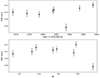 |
Fig. 6. EW of the Hγ residual line profiles ordered by HJD (top) and folded in phase (bottom). |
Interestingly, the EWs are not modulated by the orbital period and present a clear extremum at phase 0.9. A GLS periodogram identified a period of 3.29 d (f = 0.304 d−1), though with a very high FAP of approximately 0.6, preventing a definitive detection. However, this period is consistent with the signal observed at the line centre (see Fig. 4).
3.3. He i D3
The narrow component (NC) of the He i D3 line (587.6 nm) is traditionally employed to investigate the magnetospheric accretion process (e.g. Bouvier et al. 2020, 2023; Nowacki et al. 2023; Pouilly et al. 2024b). Its formation requires the hot and dense conditions found exclusively in the post-shock region of the accretion shock at the stellar surface (Beristain et al. 2001). The He i D3 lines of V4046 Sgr are shown in Fig. 7. Even though these lines are affected by low S/N and strong variability, the presence of a NC is evident at nearly all phases at the secondary's velocity. This suggests that the secondary appears to be the main accretor in the system, as also indicated by the Balmer lines (see Fig. 3).
The periodogram analysis of the line is presented in Fig. 8. In the primary's velocity reference frame, the red wing of the line is modulated at a frequency slightly lower than, but consistent with, the orbital period, with a false FAP reaching 10−3. At the line centre, where the NC of the primary is located, the frequency of modulation appears around f = 0.3 d−1 (FAP = 10−1), consistent with the signal observed in the Balmer line analysis (see Sect. 3.2). In the secondary's velocity reference frame, the signal consistent with the orbital period previously observed in the red wing is shifted towards the line centre (FAP = 10−2), and no signal around f = 0.3 d−1 with a significantly low FAP is detected.
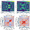 |
Fig. 8. Same as Fig. 4 (top row) and Fig. 5 (bottom row), but for the He i D3 line in the primary (left) and secondary (right) velocity frame. |
Figure 8 also presents the autocorrelation matrices of the line in both velocity reference frames. As with the Balmer lines, the matrix in the primary's velocity reference frame shows a typical SB2 modulation behaviour, with well-correlated blue and red wings that are anti-correlated with each other. In the secondary's velocity reference frame, the matrix exhibits three substructures: between −140 and −60 km s−1, between −60 and 0 km s−1, and between +20 and +75 km s−1. The negative and positive regions are likely associated with the primary emission, while the region around the line centre corresponds to the NC of the secondary.
Then we cross-correlated the He i D3 with the Hγ (see Fig. 9). When both lines are set to the primary's velocity reference frame, the typical SB2 behaviour is recovered. When the two lines are set to the secondary's velocity reference frame, the overall He i D3 line appears to be correlated with the entire blue region of Hγ. A detailed analysis of the highest correlation coefficients (>0.95) reveals that the ∼−60 km s−1 region of the He i D3 line is highly correlated with the line centre of Hγ. Additionally, two other regions of the He i D3 line, around +20 and +80 km s−1, show high correlation with the blue wing of Hγ (between −60 and −160 km s−1).
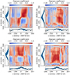 |
Fig. 9. Correlations matrices Hγ vs He i D3. Left column: Hγ set to the primary's velocity frame. Right column: Hγ set to the secondary's velocity frame. Top row: He i D3 set to the primary's velocity frame. Bottom row: He i D3 set to the secondary's velocity frame. |
When the Hγ line is set to the primary's velocity reference frame and the He i D3 line to the secondary's velocity reference frame, the correlation matrix exhibits different behaviour. A strong correlation (>0.95) is observed between the He i D3 line (at ∼−60 km s−1) and the red wing of Hγ (between +30 and +120 km s−1). The anti-correlation between the He i D3 line and the blue wing of Hγ is weaker, with coefficients around −0.7. In the opposite velocity frame configuration, only a redshifted region of the He i D3 line (around +130 km s−1) exhibits a strong correlation with the blue wing of Hγ.
Although these matrices may seem disorderly, they suggest accretion signatures in Hγ and He i D3 from both components. Some accretion occurs along the line of sight at the same time, producing the observed correlations between the line centres and the blue- and redshifted regions.
3.4. Ca ii infrared triplet
Given the limited information we could extract from the NC of the He i line, we extended our investigation by examining the Ca ii infrared triplet (IRT), located at approximately 849.8, 854.2, and 866.2 nm. Given the similar shape and variability of the three lines, we first performed an LSD-like averaging of the three lines to produce a profile that we refer to as the Ca ii IRT line for simplicity.
These lines are shown in Fig. 10 and consist of the photospheric absorption of the two components in addition to two NCs in emission, originating close to the stellar surface. Studying the NCs of the Ca ii IRT allows us to trace the accretion process of each component. Surprisingly, a 2D periodogram analysis (not shown here) did not reveal any periodicity in the NCs, whether in the primary's or secondary's velocity reference frame.
To isolate the NCs, we first performed the same double-Lorentzian profile fit as Donati et al. (2011) on the photospheric absorption, combined with a double-Gaussian profile for the NCs. We then applied the same iterative method as for the LSD profiles (see Sect. 3.1) in order to disentangle the two components and produce a mean NC for the A and the B components. Finally, we corrected the profiles using the mean NC of the B component to obtain the individual NCs of the A component, and vice versa.
We extracted the Vr of the two NCs from the disentangling procedure and fitted the corresponding curves using the method described in Pouilly et al. (2021) to constrain the emitting regions of the NCs (see Fig. 11). The results are summarised in Table 3. For the emitting region of the NC of the primary, our results are consistent within 1σ with those of Donati et al. (2011), indicating a location close to the rotation pole and facing the observer at ϕ = 0.66; the authors found 0.1, which corresponds to 0.67 in our work, but they used a different ephemeris. However, our results for the NC of the secondary deviate from those of Donati et al. (2011). While we confirm the polar location of the emitting region, it faces the observer at ϕ = 0.01, the latter authors reported ϕ = 0.82 (using our ephemeris), indicating consistency at only 2σ. The large uncertainties on the colatitudes obtained for the two components reflect an extended emitting region, also recovered by Donati et al. (2011).
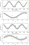 |
Fig. 11. Radial velocity fit of the Ca ii IRT NC A (two top panels) and B (two bottom panels) corrected from the Doppler velocity modulation induced by the orbital motion derived in Sect. 3.1. Each colour represents an orbital cycle. The black dash-dotted curve is the curve fitted, its uncertainty on the amplitude is represented in grey. |
Results of the fit of the Ca ii IRT NCs velocities.
The 2D periodograms of each component's NC in their respective velocity frames are shown in Fig. 12. The A component shows a signal at f = 0.5 (FAP = 10−2). The B component appears to be periodic on the same period as the orbital motion, with a fairly low FAP (10−1), although the signal seems slightly blueshifted (−25 km s−1).
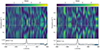 |
Fig. 12. Same as Fig. 4, but for the NC of the A (left) and B (right) components in their respective velocity reference frame. |
The aim of disentangling the two NCs was to study the EW of each NC. The plots are shown in Fig. 13, and the values are summarised in Appendix B. No periodicity was detected in the EWs. When examining the EWs of the non-disentangled NCs, two extrema are present at approximately ϕ = 0.3 and 0.8, as expected, since the two components are merged at these phases. However, for the EWs of the disentangled NCs, only the extremum at 0.3 remains, indicating that this peak is likely due to a NC feature.
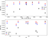 |
Fig. 13. Same as Fig. 6, but for the Ca ii IRT NCs. The black dots show the values for the combined profiles; the EWs of the primary's and secondary's NCs are displayed in blue and red, respectively. |
3.5. TESS light curves
V4046 Sgr was observed by TESS twice, in Sectors 13 and 66. The two curves of PDC SAP flux are shown in Fig. 14. We converted the BTJD to HJD by applying a shift of 69.184 s (Nelson 2023), and we folded them in phase using the ephemeris in Eq. (1). The GLS periodogram analyses yield period detections fully consistent with the orbital period. In Sector 13, an isolated flare occurs around HJD 2 458 675 (ϕ = 0.35), as well as an enhancement at phase 0.55, which reaches the maximum of luminosity modulation at the point when it should be at its minimum. However, in Sector 66, the strongest luminosity enhancement occurs around phase 0.9, on two different cycles, and well above the maximum of the modulation. Figure C.1 also displays the Sector 13 and 66 TESS light curves folded in phase, but the rotation cycles have been split and shifted vertically to improve the readability of each cycle. The phases 0.25, 0.5, and 0.75 are emphasised by vertical grey dotted lines; they represent particular points of the orbit following the ephemeris in Eq. (1). Indeed, ϕ = 0.25 is the point when the radial velocity of the primary switches from negative to positive values (with respect to the systemic velocity), meaning that this component is in front of the observer and the secondary is behind, from phases 0.0 to 0.5. Phase 0.75 represents the opposite situation, meaning that the secondary is in front of the observer from phases 0.5 to 1.0. We note that, given the low inclination of the orbit (∼35°), no eclipse occurs and both components are visible at all phases; the two conjunctions only indicate which component is the closest to the observer. The phased light curve seems to be a superposition of a typical sinusoidal binary modulation (see cycles 1483 and 2082), with punctual luminosity enhancements due to the accreting component during the different orbital cycles. However, the minimum of the modulation is slightly offset from phase 0.25, and the maximum from phase 0.75, as expected if one component is less bright than the other. Furthermore, the two components have very similar temperatures; the literature values indicate that the hottest one is the primary, with a K5 spectral type, while the secondary is K7 (Quast et al. 2000). Assuming a blackbody emission, this means that the minimum should occur at phase 0.75 and the maximum at phase 0.25. The sinusoidal modulation observed is thus likely due to a spot on one of the components. For the superimposed punctual luminosity enhancements we find the following: during cycles 1479 and 1480 (Sector 13), the light curve shows multiple luminosity peaks around phase 0.25, meaning that they represent accretion events on the primary during this cycle. However, cycles 1486 and 1487 show an overall luminosity increase centred on phase 0.75, reflecting an accretion event on the secondary. When the multiple peaks of these events on the primary indicate a discrete accretion pattern, the process on the secondary seems more continuous, distorting the symmetry of the sinusoidal shape of the modulation. This behaviour is confirmed in Sector 66, with multiple luminosity peaks on the primary ‘side’ of the phased curve (cycles 2078, 2079), and a more continuous enhancement on the secondary side (cycles 2074, 2083).
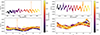 |
Fig. 14. Sector 13 (left) and 66 (right) TESS light curves (top panels), folded in phase following Eq. (1) (bottom panels). The colour scale indicates the HJDs. |
4. Discussion
V4046 Sgr was selected for this study due to the intriguing contradiction between its highly ordered configuration–two components with similar masses, ages, and temperatures, in a circularised orbit with synchronised rotation–and its chaotic accretion process, as reported in prior studies. While the ESPaDOnS spectropolarimetric time series allowed Donati et al. (2011) to derive the magnetic field topology of the system, no detailed description of its accretion pattern was provided, despite the suitability of such a dataset for this purpose (e.g. Pouilly et al. 2020, 2021, 2023, 2024a, b). This work seeks to address this gap.
We first derived the LSD profiles of V4046 Sgr to extract the radial velocity modulation of the system and determine its orbital parameters. Our results are fully consistent with those of Stempels & Gahm (2004), although using their ephemeris would result in a 0.069-cycle shift for conjunctions (Donati et al. 2011). This discrepancy was corrected using the orbital parameters derived in this work, which we used to define the ephemeris (Eq. 1), despite the larger uncertainties.
Our analysis confirmed accretion onto both components, as evidenced by the emission line peaks at the velocities of the Balmer lines (tracing accretion funnel flows), Ca ii IRT NC and He i NC (formed near the accretion shock, Beristain et al. 2001). However, we identified significantly different accretion patterns between the two components, as revealed by the variability in line profiles when analysed in the reference frame of each star.
4.1. Primary component (V4046 Sgr A)
An IPC profile in Hγ at phases 0.33 and 0.37, extending up to +350 km s−1, indicates the presence of an accretion funnel flow. This signature is attributed to the primary based on the line region's periodicity consistent with its rotation period (Fig. 4) and its clear and separated correlation in the autocorrelation matrix when set to the primary's velocity reference frame (Fig. 5). According to the magnetospheric accretion scheme for cTTSs (see review by Hartmann et al. 2016), such a funnel flow should channel material onto the stellar surface near the dipole pole, forming an accretion shock.
For V4046 Sgr A, this is consistent with the dipole pole's location at ϕ = 0.37 (Donati et al. 2011, using our ephemeris), in phase with the IPC profile and the minimum Ca ii IRT NC EW. Furthermore, the TESS light curves (Fig. 14) reveal multiple accretion-induced luminosity peaks near the time of the primary's conjunction, likely caused by a discrete accretion flow separated into sub-arms, as observed in systems like V807 Tau (Pouilly et al. 2021).
4.2. Secondary component (V4046 Sgr B)
The accretion onto the secondary appears less structured than that onto the primary. The He i D3 NC indicates the presence of an accretion shock at the stellar surface, periodic with the orbital period, and suggests that V4046 Sgr B is the system's main accretor, because it is mostly located at the seconary's velocity. However, the Hγ EW, thus expected to be dominated by the secondary, shows no periodicity consistent with the rotation period, and its autocorrelation matrix does not exhibits the behaviour expected from the magnetospheric accretion scheme.
None of the diagnostics aligns with the dipole pole of the secondary (ϕ≈0.6 using our ephemeris, Donati et al. 2011). Moreover, the TESS light curves show an overall luminosity enhancement at the phases of the secondary's conjunction, indicating a less concentrated accretion structure compared to the primary.
4.3. Dissimilar accretion patterns
This work demonstrates different accretion onto the two components of V4046 Sgr. While surprising given their similarities, this difference is consistent with their distinct magnetic topologies. V4046 Sgr's evolutionary stage, slightly more advanced than typical cTTSs, has resulted in the development of radiative cores and complex magnetic topologies (Donati et al. 2011).
Both stars exhibit weak large-scale magnetic fields, with significant toroidal, quadrupolar, and octupolar components, deviating from the strong poloidal and dipole fields typically observed in cTTSs. Despite this complexity, magnetospheric accretion can still occur, as seen in HQ Tau (Pouilly et al. 2020). However, the obliquities of the magnetic dipole axes (60° for V4046 Sgr A and roughly 90° for V4046 Sgr B) are unusually high compared to the 5 to 20° range observed in cTTSs with stable accretion (McGinnis et al. 2015). Dipole magnetic obliquity is a key parameter affecting directly the magnetospheric radius, which means the limit between a stable regime, where an accretion funnel flow connects the disc to the stellar dipole pole, and an unstable one, characterised by accretion tongues penetrating the magnetosphere and connecting the disc to the stellar equator (Romanova & Owocki 2015).
4.4. Magnetospheric radii and accretion regimes
Using the values from Donati et al. (2011), the magnetospheric radii are 0.82 ± 0.67 R★ and 0.09 ± 0.08 R★ for the primary and secondary (using 89° instead of 90°, which brings the value down to 0), respectively. For V4046 Sgr B, the nearly perpendicular dipole field likely prevents stable magnetospheric accretion, as its magnetospheric radius does not reach the stellar surface in the disc's plane.
The primary's magnetospheric radius cannot directly truncate the circumbinary disc (located at ∼10 R★, Stempels & Gahm 2004). However, the gas bulks detected in the Roche lobes, near the co-linear Lagrangian points, at ∼6.93 R⊙ from the system's centre of mass (meaning at ∼1.15 R★ from the stars), could allow material to be channelled to the stellar surface via the magnetosphere. This is reminiscent of the accretion scheme of DQ Tau and AK Sco (Pouilly et al. 2023, 2024a, respectively), where magnetospheric accretion is ongoing on the components surrounded by a circumbinary disc that is too far away to be directly truncated by the magnetic field.
4.5. Other periodicity detected in accretion structures
A tentative periodicity of f≈0.3 d−1 (∼3.3 days) was detected in the Balmer line centres, the Hγ EW modulation, and the He i D3 NC (in the primary's velocity reference frame). This periodicity indicates that the ESPaDOnS time series covers only two periods. Furthermore, the EW of Hγ in Fig. 6 appears relatively stable, with the exception of an extremum at HJD 2 455 081.72. This value, likely due to a flare also reported by Donati et al. (2011), may be responsible for the detection of the 3.3-day period. To verify the validity of this period, we first generated a 3.3-day periodic signal (sine wave), sampled at the observation dates, to confirm the sampling allowed for the detection of this period. A GLS periodogram analysis successfully recovered the periodicity, with a FAP of 10−3. We then performed a leave-one-out test on the Hγ flux in the velocity channel where the minimum FAP was achieved. This involved iteratively removing one observation from the dataset and computing the associated periodogram and FAP. All eight periodograms showed a peak between 0.29 and 0.31 d−1, with a FAP between 10−1 and 10−2. These tests demonstrate that the 3.3-day periodicity is genuinely detected and not solely induced by the flare at HJD 2 455 081.72.
This periodicity likely corresponds to accretion structures cycling through the line of sight, but does not match any harmonic of the rotation period. We suspect this behaviour to be implied by two different structures, for example two accretion funnel flows with two associated accretion shocks, the second appearing on the line of sight ∼0.9 d (0.37 rotation cycle) after the first. This would implies a delay of 3.3 d between the first appearance of the structure #1 and the second appearance of structure #2, and between the second passage of structure #1 and the third of structure #2, yielding the detection of the 3.3-day period. We propose two scenarios:
-
–
Accretion tongue on the primary (Fig. 15): A secondary accretion tongue penetrates the primary's magnetosphere to reach the stellar surface at phase 0.66, and the emitting region of the Ca ii IRT NC (see Sect. 3.4). Together with the accretion funnel flow at phase 0.37 producing the IPC profile in Hγ and the minimum EW of the Ca ii IRT NC, this would imply a 0.29 phase shift between the two structures, only 4.7 min away from the aforementioned 0.9-day shift.
-
–
Accretion tongue on the secondary (Fig. 16): An accretion tongue connects the secondary to its associated bulk of gas, reaching the stellar surface at phase 0.01, the emitting region of its Ca ii IRT NC (see Sect. 3.4). The phase shift between such a structure and the accretion funnel flow of V4046 Sgr A is 0.36 very close to the 0.9 d mentioned above; their successive passage could thus imply the 3.3-day period detected.
Given that the 0.3 d−1 periodicity is predominantly detected when using the primary's velocity reference frame, we could favour the first hypothesis. However, the accretion is likely originating from the bulk of gas identified by Stempels & Gahm (2004), implying a single direction of infall towards the stellar surface. The first hypothesis thus suggests that the accretion tongue spirals around the star for approximately 0.8π radians from the bulk of gas to the stellar surface, and in the direction opposite to the star's rotation. While this behaviour is observed in the chaotic accretion regime simulations of Romanova & Owocki (2015), it is not characteristic of the ordered chaotic regime, which involves accretion funnel flows following magnetic field lines and accretion tongues penetrating the magnetosphere.
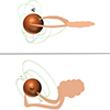 |
Fig. 15. Sketch representing the first hypothesis for the 0.3 d−1 period detected where the primary shows both an accretion funnel flow and an accretion tongue. The top panel shows the side view, the bottom panel represents the polar view. The grey line or cross is the rotation axis, the green cross is the dipole pole, the green lines are the dipole magnetic field lines. The cloud represents the bulk of gas mentioned in Sect. 4. |
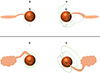 |
Fig. 16. Same as Fig. 16, but for the second hypothesis. The 0.3 d−1 period is induced here by the simultaneous passages of the accretion funnel flow of the primary and an accretion tongue on the secondary. |
Under the second hypothesis, the material spirals for only 0.5π radians, still counter-rotating, but as the secondary appears to be in a chaotic accretion regime, we currently favour this explanation.
5. Conclusions
In this paper we presented the analysis of the accretion process in V4046 Sgr, a binary system surrounded by a circumbinary disc and composed of two similar cTTSs in a circularised orbit with synchronised rotation. The aim of this study was to build on our previous efforts with DQ Tau and AK Sco to understand the accretion processes in young multiple systems by systematically accounting for the stellar magnetic field. Specifically, we sought to explore how the magnetospheric accretion process observed in single cTTSs, where a strong dipolar magnetic field truncates the disc and forces material to leave the disc plane that free-fall onto the stellar surface along magnetic field lines, can be extended to systems with higher multiplicity.
We analysed an ESPaDOnS spectropolarimetric time series that was previously studied by Donati et al. (2011) and Hahlin & Kochukhov (2022) in the context of the system's magnetic field. Given the pivotal role of magnetic fields in the accretion processes of cTTSs, these prior works provide a foundation for our complete and detailed characterisation of the accretion process in V4046 Sgr.
Our findings reveal an uneven accretion process between the two components of the system, originating from bulks of gas located near the co-linear Lagrangian points, rather than directly from the circumbinary disc. V4046 Sgr A displays clear signatures of magnetospheric accretion, primarily inferred from the IPC profiles detected in the Balmer lines and from the variations in the primary's NC of the Ca ii IRT line. These features trace an accretion funnel flow and accretion shock in phase with the primary's dipole pole.
In contrast, the secondary component does not exhibit such behaviour. However, variations in the Balmer lines and the He i D3 line indicate that this component is the main accretor of the system.
The extensive emitting regions of the NCs of the Ca ii IRT lines for both components suggest that accretion is occurring across a wide area of the stellar surfaces, rather than being confined to the concentrated locations expected for typical magnetospheric accretion processes. Consequently, we conclude that the primary operates under an ordered chaotic accretion regime, where accretion funnel flows (connecting the disc to the star's dipole pole) coexist with accretion tongues (penetrating the magnetosphere to reach the stellar surface near the equator).
For the secondary, we suspect a chaotic accretion regime, characterised exclusively by accretion tongues, consistent with its highly inclined dipole field.
Acknowledgments
We thank the anonymous referee, whose comments help in improving the strength of our work. This research was funded in whole or in part by the Swiss National Science Foundation (SNSF), grant number 217195 (SIMBA). Based on observations obtained at the Canada-France-Hawaii Telescope (CFHT) which is operated from the summit of Maunakea by the National Research Council of Canada, the institut National des Sciences de l’Univers of the Centre National de la Recherche Scientifique of France, and the University of Hawaii. The observations at the Canada-France-Hawaii Telescope were performed with care and respect from the summit of Maunakea which is a significant cultural and historic site. This work has made use of the VALD database, operated at Uppsala University, the Institute of Astronomy RAS in Moscow, and the University of Vienna. The SpecpolFlow package is available at https://github.com/folsomcp/specpolFlow. The PySTEL(L)A package is available at https://github.com/pouillyk/PySTELLA.
References
- Argiroffi, C., Maggio, A., Montmerle, T., et al. 2012, ApJ, 752, 100 [NASA ADS] [CrossRef] [Google Scholar]
- Baluev, R. V. 2008, MNRAS, 385, 1279 [Google Scholar]
- Beristain, G., Edwards, S., & Kwan, J. 2001, ApJ, 551, 1037 [Google Scholar]
- Bouvier, J., Alecian, E., Alencar, S. H. P., et al. 2020, A&A, 643, A99 [EDP Sciences] [Google Scholar]
- Bouvier, J., Sousa, A., Pouilly, K., et al. 2023, A&A, 672, A5 [NASA ADS] [CrossRef] [EDP Sciences] [Google Scholar]
- Donati, J. -F. 2003, ASP Conf. Ser., 307, 41 [NASA ADS] [Google Scholar]
- Donati, J. -F., Semel, M., Carter, B. D., Rees, D. E., & Collier Cameron, A. 1997, MNRAS, 291, 658 [NASA ADS] [CrossRef] [Google Scholar]
- Donati, J. F., Gregory, S. G., Montmerle, T., et al. 2011, MNRAS, 417, 1747 [CrossRef] [Google Scholar]
- Donati, J. F., Hébrard, E., Hussain, G. A. J., et al. 2015, MNRAS, 453, 3706 [Google Scholar]
- Gustafsson, B., Edvardsson, B., Eriksson, K., et al. 2008, A&A, 486, 951 [NASA ADS] [CrossRef] [EDP Sciences] [Google Scholar]
- Hahlin, A., & Kochukhov, O. 2022, A&A, 659, A151 [NASA ADS] [CrossRef] [EDP Sciences] [Google Scholar]
- Hartmann, L., Hewett, R., & Calvet, N. 1994, ApJ, 426, 669 [Google Scholar]
- Hartmann, L., Herczeg, G., & Calvet, N. 2016, ARA&A, 54, 135 [Google Scholar]
- Kastner, J. H., Sacco, G. G., Montez, R., et al. 2011, ApJ, 740, L17 [Google Scholar]
- Martinez-Brunner, R., Casassus, S., Pérez, S., et al. 2022, MNRAS, 510, 1248 [Google Scholar]
- McGinnis, P. T., Alencar, S. H. P., Guimarães, M. M., et al. 2015, A&A, 577, A11 [NASA ADS] [CrossRef] [EDP Sciences] [Google Scholar]
- Muzerolle, J., Calvet, N., & Hartmann, L. 2001, ApJ, 550, 944 [Google Scholar]
- Nelson, R. H. 2023, New Astron., 98, 101901 [Google Scholar]
- Nowacki, H., Alecian, E., Perraut, K., et al. 2023, A&A, 678, A86 [NASA ADS] [CrossRef] [EDP Sciences] [Google Scholar]
- Offner, S. S. R., Moe, M., Kratter, K. M., et al. 2023, ASP Conf. Ser., 534, 275 [NASA ADS] [Google Scholar]
- Pouilly, K., Bouvier, J., Alecian, E., et al. 2020, A&A, 642, A99 [NASA ADS] [CrossRef] [EDP Sciences] [Google Scholar]
- Pouilly, K., Bouvier, J., Alecian, E., et al. 2021, A&A, 656, A50 [NASA ADS] [CrossRef] [EDP Sciences] [Google Scholar]
- Pouilly, K., Kochukhov, O., Kóspál, Á., et al. 2023, MNRAS, 518, 5072 [Google Scholar]
- Pouilly, K., Hahlin, A., Kochukhov, O., Morin, J., & Kóspál, Á. 2024a, MNRAS, 528, 6786 [NASA ADS] [CrossRef] [Google Scholar]
- Pouilly, K., Audard, M., Kóspál, Á., & Lavail, A. 2024b, A&A, 691, A18 [NASA ADS] [CrossRef] [EDP Sciences] [Google Scholar]
- Quast, G. R., Torres, C. A. O., de La Reza, R., da Silva, L., & Mayor, M. 2000, IAU Symp., 200, 28 [NASA ADS] [Google Scholar]
- Romanova, M. M., & Owocki, S. P. 2015, Space Sci. Rev., 191, 339 [Google Scholar]
- Ryabchikova, T., Piskunov, N., Kurucz, R. L., et al. 2015, Phys. Scr., 90, 054005 [Google Scholar]
- Stempels, H. C., & Gahm, G. F. 2004, A&A, 421, 1159 [NASA ADS] [CrossRef] [EDP Sciences] [Google Scholar]
Appendix A: Radial velocities
Here we provide the radial velocities derived for each components and for each observation using our disentangling method of LSD Stokes I profiles. This method is described in Sect. 3.1 and the curve is shown in Fig. 2.
Radial velocities obtained from the LSD Stokes I disentangling procedure (see Sect. 3.1).
Appendix B: Equivalent widths
In this Appendix we present a table summarising the EWs described in Sect. 3.
Equivalent widths of lines computed in this work.
Appendix C: TESS light curves folded in phase
In this appendix we provide another visualisation of the TESS light curves shown in Fig. 14. Here only the curves folded in phase are presented, but each cycle has been shifted vertically to better appreciate the individual variabilities.
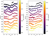 |
Fig. C.1. Sector 13 (left) and 66 (right) TESS light curves folded in phase following Eq. 1. The different cycles have been shifted vertically to improve the readability. The vertical grey dotted lines illustrate the phase 0.25 (component A is in front of the observer), 0.5, and 0.75 (component B is facing the observer). The y-axis labels denote the orbital cycle from the first ESPaDOnS observation used in this work. |
All Tables
Radial velocities obtained from the LSD Stokes I disentangling procedure (see Sect. 3.1).
All Figures
|
Fig. 1. LSD Stokes I profiles of V4046 Sgr. The blue (red) ticks illustrate the velocity of the A (B) component. The orbital phases (computed from Eq. 1) and HJDs (−2 450 000 d) are indicated respectively on the left and right of each profile. |
| In the text | |
|
Fig. 2. Radial velocity curves of the primary (blue) and secondary (red) components of V4046 Sgr. The top panel represents velocity as function of the HJD, while the bottom panel shows the curve folded in phase using the ephemeris of Eq. (1). The dash-dotted curve shows the orbital solution using the parameters of Table 2. The error bars are included in this plot, but are smaller than the marker sizes. |
| In the text | |
|
Fig. 3. Hα (left two pannels), Hβ (middle two panels), and Hγ (right two panels) residual profiles of V4046 Sgr. These profiles are ordered by orbital phase and corrected from the radial velocity of the primary. The red ticks indicate the velocity of the secondary. The orbital phases and HJDs are indicated respectively on the left and right of each profile. |
| In the text | |
|
Fig. 4. 2D periodograms of Hα (left), Hβ (middle), and Hγ (right) residual lines in the primary's (top row) and secondary's (bottom row) velocity frame. The colour scales the power of the periodogram and the white dotted line highlights the orbital period. The mean profile and it variance are shown at the bottom of each plot in black and blue, respectively. The mirroring effect is due to the one-day aliasing, a spectral leakage of the Fourier transform reproducing, with the real signal, the observation sampling. The signal and its alias are disentangled thanks to the FAP. |
| In the text | |
|
Fig. 5. Hγ residual line autocorrelation matrix in the velocity frame of the primary (left) and secondary (right). The colour-code scales the correlation coefficient: red represents a strong correlation and blue shows a strong anti-correlation. The plots along the x- and y-axes represent the corresponding mean line profile (black) and its variance (blue). |
| In the text | |
|
Fig. 6. EW of the Hγ residual line profiles ordered by HJD (top) and folded in phase (bottom). |
| In the text | |
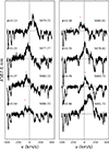 |
Fig. 7. Same as Fig. 3, but for the He i D3 line. |
| In the text | |
|
Fig. 8. Same as Fig. 4 (top row) and Fig. 5 (bottom row), but for the He i D3 line in the primary (left) and secondary (right) velocity frame. |
| In the text | |
|
Fig. 9. Correlations matrices Hγ vs He i D3. Left column: Hγ set to the primary's velocity frame. Right column: Hγ set to the secondary's velocity frame. Top row: He i D3 set to the primary's velocity frame. Bottom row: He i D3 set to the secondary's velocity frame. |
| In the text | |
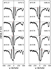 |
Fig. 10. Same as Fig. 3, but for the Ca ii IRT line profiles. |
| In the text | |
|
Fig. 11. Radial velocity fit of the Ca ii IRT NC A (two top panels) and B (two bottom panels) corrected from the Doppler velocity modulation induced by the orbital motion derived in Sect. 3.1. Each colour represents an orbital cycle. The black dash-dotted curve is the curve fitted, its uncertainty on the amplitude is represented in grey. |
| In the text | |
|
Fig. 12. Same as Fig. 4, but for the NC of the A (left) and B (right) components in their respective velocity reference frame. |
| In the text | |
|
Fig. 13. Same as Fig. 6, but for the Ca ii IRT NCs. The black dots show the values for the combined profiles; the EWs of the primary's and secondary's NCs are displayed in blue and red, respectively. |
| In the text | |
|
Fig. 14. Sector 13 (left) and 66 (right) TESS light curves (top panels), folded in phase following Eq. (1) (bottom panels). The colour scale indicates the HJDs. |
| In the text | |
|
Fig. 15. Sketch representing the first hypothesis for the 0.3 d−1 period detected where the primary shows both an accretion funnel flow and an accretion tongue. The top panel shows the side view, the bottom panel represents the polar view. The grey line or cross is the rotation axis, the green cross is the dipole pole, the green lines are the dipole magnetic field lines. The cloud represents the bulk of gas mentioned in Sect. 4. |
| In the text | |
|
Fig. 16. Same as Fig. 16, but for the second hypothesis. The 0.3 d−1 period is induced here by the simultaneous passages of the accretion funnel flow of the primary and an accretion tongue on the secondary. |
| In the text | |
|
Fig. C.1. Sector 13 (left) and 66 (right) TESS light curves folded in phase following Eq. 1. The different cycles have been shifted vertically to improve the readability. The vertical grey dotted lines illustrate the phase 0.25 (component A is in front of the observer), 0.5, and 0.75 (component B is facing the observer). The y-axis labels denote the orbital cycle from the first ESPaDOnS observation used in this work. |
| In the text | |
Current usage metrics show cumulative count of Article Views (full-text article views including HTML views, PDF and ePub downloads, according to the available data) and Abstracts Views on Vision4Press platform.
Data correspond to usage on the plateform after 2015. The current usage metrics is available 48-96 hours after online publication and is updated daily on week days.
Initial download of the metrics may take a while.