| Issue |
A&A
Volume 698, June 2025
|
|
|---|---|---|
| Article Number | A198 | |
| Number of page(s) | 12 | |
| Section | Planets, planetary systems, and small bodies | |
| DOI | https://doi.org/10.1051/0004-6361/202553905 | |
| Published online | 17 June 2025 | |
Context images for Venus Express radio occultation measurements: A search for a correlation between temperature structure and UV contrasts in the clouds of Venus
1
Lightcurve Films,
Portugal
2
AOPP, University of Oxford,
UK
3
European Space Agency,
ESTEC,
Noordwijk,
The Netherlands
4
Department of Astronomy, University of Michigan,
Ann Arbor,
USA
5
Rheinisches Institut für Umweltforschung, Universität zu Köln,
Germany
6
Planetary Atmospheres Group, Institute for Basic Science (IBS),
Daejeon,
South Korea
7
Space Research Institute of the Russian Academy of Sciences (IKI),
Moscow,
Russia
★ Corresponding author: This email address is being protected from spambots. You need JavaScript enabled to view it.
Received:
27
January
2025
Accepted:
28
April
2025
Abstract
Context. Venus exhibits strong and changing contrasts at ultraviolet wavelengths. They appear to be related to the clouds and the dynamics in the cloud layer, but to date their origin continues to be unknown.
Aims. We investigate the nature of the UV contrasts exhibited by Venus’ clouds by examining possible correlations between the thermal structure inferred from radio occultation data and UV brightness from imagery data, both observed with Venus Express.
Methods. We analysed Venus Express images obtained from 11 hours before to a few hours after the time of radio occultation measurements of the same area. We accounted for the advection of clouds by zonal and meridional winds and applied a phase angle correction to compensate for the changing viewing geometry.
Results. We find a possible anti-correlation between UV brightness and atmospheric temperature around an altitude of 67 km for low latitudes, with a one percent probability of this finding being due to chance (p value = 0.01). Heating in this altitude and latitude region due to an increase in the UV absorber has been predicted by radiative forcing studies. The predictions roughly match our observed temperature amplitude between UV-dark and UV-bright regions.
Conclusions. This could be the first observational evidence of a direct link between UV brightness and atmospheric temperature in the 65–70 km altitude region in the clouds of Venus.
Key words: planets and satellites: atmospheres / planets and satellites: general
© The Authors 2025
 Open Access article, published by EDP Sciences, under the terms of the Creative Commons Attribution License (https://creativecommons.org/licenses/by/4.0), which permits unrestricted use, distribution, and reproduction in any medium, provided the original work is properly cited.
This article is published in open access under the Subscribe to Open model. This email address is being protected from spambots. You need JavaScript enabled to view it. to support open access publication.
1 Introduction
Venus is completely enveloped by highly reflective clouds. The upper clouds are composed mainly of sulphuric acid. At visible and infrared wavelengths, the Venus clouds look very homogeneous. However, there are strong contrasts at UV wavelengths, which were first observed in the early twentieth century (Wright 1927; Ross 1928). Ross (1928) suggested that these UV contrasts might be correlated to temperature differences between the north and south halves of Venus, which he based on temperature estimates derived from broad-band IR emission measurements reported by Coblentz & Lampland (1925). Significant UV absorption at wavelengths below 300 nm is due to sulphur dioxide, especially at lower latitudes, and ozone at latitudes polewards of ±50° (Marcq et al. 2019). An additional UV-to-blue absorber, or absorbers, is required at 300–450 nm to match the observed spectrum (Pollack et al. 1980; Marcq et al. 2020). The chemical identity of this UV-to-blue-absorber is still unknown. Proposed compositions include a mixture of elemental sulphur allotropes (Toon et al. 1982), ferric chloride (Esposito et al. 1997), and disulphur dioxide (Frandsen et al. 2016). Concerning the vertical distribution, measurements from descent probes concur that the UV-to-blue absorber lies above 57 km (Tomasko et al. 1980; Ekonomov et al. 1984), but show that the peak absorption must be just under the cloud top level in the 66–73 nm altitude range (Crisp 1986; Lee et al. 2015b) to explain the observed phase angle dependence of the contrast (Pollack et al. 1980) and the mean phase curve of the disc brightness (Lee et al. 2021).
Just as the identity of the UV-to-blue-absorber is unknown, the reasons for the UV contrasts are also unknown. Titov et al. (2008) infer from data of the Venus Express/VIRTIS instrument that UV contrast changes are associated with upwelling from below and not with changes in the top cloud altitude. However, it is not clear whether the upwelling advects UV-dark material such as poly sulphur or  , or UV-bright material such as sulphuric acid haze particles, which are more spatially variable. If the contrasts are associated with upwelling in the cloud layer, the question is whether this upwelling brings UV-dark material or UV-bright haze-forming material to the cloud tops, or whether upwelling brings progenitor species to the cloud tops, which could be UV-dark, UV-bright, or UV-neutral. Cottini et al. (2015) present a search for correlations between the cloud top altitude measured at 2.5 micron wavelength from Venus Express VIRTIS-H spectra, and the UV brightness measured simultaneously by VIRTIS-M between 375 nm and 385 nm, and report that there might be some anti-correlation with darker UV areas corresponding to higher cloud tops (denser clouds), but it is not systematic (their Fig. 8). Patsaeva et al. (2015) use altimetry from VIRTIS-M for VMC UV images and show that cloud motion vectors obtained for darker regions lying 1–1.5 km above adjacent bright regions give a different horizontal flow direction (their Fig. 11). Lee et al. (2020) report on a clear anticorrelation between the overall brightness of Venus at 283 nm (SO2 absorption) and 365 nm (unknown absorber) and at 2.02 micron in several years of Akatsuki data. The 2.02 micron wavelength area is very sensitive to cloud top height, because it is strongly affected by carbon-dioxide absorption.
These are mechanisms by which temperature contrasts and dynamics could lead to changes in the UV brightness. However, the UV-to-blue-absorber also has radiative effects; in particular, UV-dark regions should be expected to absorb more sunlight, at least in the UV part of the spectrum, and thus might be expected to experience higher temperatures than UV-bright regions. The present analysis of co-located UV imagery and radio occultation measurements could provide constraints on the vertical distribution of UV absorption and validation of previous calculations of UV-contrast-related heating rates (Crisp 1986; Lee et al. 2019).
The Venus Express mission (Svedhem et al. 2007) produced very useful and unique datasets. From the radio occultation data obtained with the VEnus RAdio science (VeRa) experiment, vertical density profiles of the atmosphere can be derived with a high vertical resolution. Pressure and temperature profiles can be calculated from these profiles by integration and the assumption of hydrostatic balance (Tellmann et al. 2009). The cloud contrasts are most easily observed in images obtained with the UV channel of the Venus Monitoring Camera (VMC), which has a bandpass centred at a wavelength of 365 nm at the peak of the unknown UV absorption (Markiewicz et al. 2007). The Visible and InfraRed Thermal Imaging Spectrometer (VIRTIS) instrument obtained hyperspectral images that include coverage of the UV feature, but are not favoured in this analysis for two reasons: first, there are far fewer UV VIRTIS images than there are UV VMC images, and they cover a smaller area due to the smaller field of view; second, the VIRTIS UV-VIS channel suffers from stray light problems at wavelengths below 500 nm that are not yet fully resolved. On the other hand, VIRTIS-IR observations offer two relevant observational constraints on cloud processes: (1) dayside observations of CO2 line depths measure the height of the cloud tops at these wavelengths (Ignatiev et al. 2009); and (2) nightside observations in 1.7 and  windows offer the possibility to constrain lower cloud optical thicknesses (Barstow et al. 2012).
In the present study, we identify orbits during which both VeRa radio occultation sounding and VMC imaging were done. We look for correlations between the VeRa temperature profile and static stability with UV brightness measured by VMC. The observations and analysis procedure are described in Section 2, followed by an analysis of the results and a discussion in Section 3. We did assess the possibility of studying correlations using VIRTIS nightside imagery, but too few co-located observations were found for a meaningful analysis to be done. We also looked into the SPICAV-UV dataset. We found that this set does not have significant overlap in time and location with the VMC and VeRa datasets.
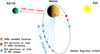 |
Fig. 1 Schematic of Venus Express orbit around Venus with VMC imaging happening on ingress and egress (blue dots) and VeRa radio occultation shortly after periapsis (red dot). |
2 Data and reduction
2.1 Selection of observations
Venus Express was equipped with two High Gain antennae, pointing in directions nearly aligned with the spacecraft’s  and −X axes, respectively. The VMC instrument boresights, on the other hand, were directed in the +Z direction. Hence, there could never be any observations of the same location by VMC and VeRa simultaneously. To obtain imagery of a VeRa sounding location, it would have been necessary to slew the spacecraft before or after the VeRa sounding. For observations of the northern hemisphere, the spacecraft’s altitude above the clouds was too low, and hence the spacecraft velocity too high, to make this feasible. It was possible to obtain observations of the southern hemisphere when the spacecraft was much further from the planet and moving at much lower orbital velocities.
A dedicated South Polar Dynamics Campaign (SPDC) was carried out between 25 November and 31 December 2013, designed to allow imagery of VeRa sounding locations (orbit numbers 2775 through 2811, last section in Table A.1). On each orbit one VeRa atmospheric sounding was acquired shortly after the pericentre passage at high southern latitudes  to
to  . Before and after the VeRa sounding, the VMC camera boresight was pointed at the planet and images were taken. On ingress VMC acquired images at half-hourly intervals over a period of several hours. The geometry of the observations is shown schematically in Fig. 1. After pericentre a brief period of about one hour was available for imaging. For 30 orbits from the SPDC, good data from both VeRa and VMC are available, separated in time by less than 12 hours.
During the rest of the Venus Express mission, VMC images of Venus containing VeRa sounding locations within a few hours of the sounding had not been planned, but do occur. We identified an additional 26 orbits during which co-located VeRa and VMC data are available and usable for analysis. These cover the VEX mission extensions 2 through 4, starting at orbit number 1191. By including these observations, we extended our analysis over a wider range of southern latitudes. All the selected observations are listed in Table A. 1 and the distribution of the VeRa profiles on Venus is shown in Fig. 2 as a function of latitude, longitude, and local solar time.
2.2 VeRa dataset
The VeRa experiment and data are described in detail in Pätzold et al. (2007) and Tellmann et al. (2009). The processed VeRa datasets consist of density, pressure, and temperature profiles of the neutral atmosphere from approximately 50 to 100 km in altitude. The vertical resolution of VeRa temperature profiles depends on observation geometry, but is typically of the order of several hundred metres. For our analysis we applied a binning scheme for each profile: we calculated the average value of the VeRa temperatures and pressures inside  bins between 46 and 102 km altitude. This is equivalent to applying a low pass filter and also helps to minimise any effects of gravity waves on our data and consequently our analysis. We discuss gravity waves in more detail below.
In Figs. 3a–c, we show an example of such a binned profile, compared to its full profile. We also computed the temperature gradient (Fig. 3d) and static stability profiles S(z) for each temperature profile (Fig. 3f). Static stability is defined as the observed temperature gradient rate minus the adiabatic lapse rate: we derived the adiabatic lapse rates from Figure 18 in Seiff et al. (1980) (Fig. 3e) and calculated  at 1 km intervals, as is shown in Fig. 3f. A sharp change in regime can be seen from a low stability, indicating convective overturning in the lower cloud deck between 50 and 60 km altitude, to a high-stability upper cloud layer extending upwards from 60 km altitude. In the present study, we look for correlations between the UV brightness and both temperature and static stability at all relevant altitudes.
Particular care should be taken with analysing radio occultation temperature data when strong inversions are present, which can occur at high latitudes near the tropopause around 60 km . In this case the radio signal may take multiple paths through the atmosphere, causing an error in the retrieved temperature profile of  in magnitude (Herrmann et al. 2014). Corrections for multi-path effects are not routinely available at the time of writing and were not used in the present analysis. We note that it may introduce errors in the temperature profile in the
  altitude range, at high latitudes poleward of
  . This is below the altitude range targeted in this analysis is
  and 17 out of 56 profiles assessed in this work were obtained at latitudes higher than
  (Table A.1).
There are also known effects on the temperature structure at and above the cloud level due to thermal tides and gravity waves. These effects have been studied by many authors with data from different Venus missions. Zasova et al. (2007) and Imamura et al. (2018) presented an analysis of Venus Express data, Kouyama et al. (2017), Imamura et al. (2018) and Akiba et al. (2021) presented an analysis of Akatsuki data. Thermal tides are a function of latitude and local solar time. Akiba et al. (2021) present amplitudes of these tides as a function of latitude and altitude. The altitude range, however, is limited between 65 and 72 km , in the range of the focus of our analysis between 65 and 75 km in altitude. The reported thermal tide amplitudes are in the  range, of the order of the uncertainties in the temperature values in our analysis (Fig. 3b). To evaluate the effect of applying a thermal tide correction, we took the available data for Figure 5 in Akiba et al. (2021) from the corresponding Zenodorepository. This data is for the 69 km altitude level. We extracted thermal tide amplitudes for the latitudes and local solar times of the VeRa soundings that we used. We performed the statistical analysis, described in detail in Section 3, with and without the correction for the thermal tide. The resulting values for the Pearson and Spearman correlation coefficients for the three latitude bins that we defined (low, mid, and high latitude, see Section 3) are the same within the uncertainties. Hence, we decided that attempting to correct for the thermal tide was not necessary for the data we used and the way we analysed it.
The exact origin of gravity waves in the atmosphere of Venus is still under debate. Tellmann et al. (2012) report on smallscale temperature fluctuations of up to  derived from the analysis of VeRa data from all over Venus. They observe the onset of wavelike temperature fluctuations at around 60 km in altitude, the tropopause in the middle of the cloud layers. Here the atmosphere changes from an adiabatic to convectively stable state, with excursions back to adiabatic in thin confined layers throughout the cloud layer. The amplitude of the temperature fluctuations diminishes with altitude all the way up to 90 km . Towards the latitudes of
  , the polar collar regions, the overall amplitudes of the temperature fluctuations are larger. At this latitude the polar collar is observed, with much lower tropopause temperatures, a phenomenon that is not yet fully understood. Imamura et al. (2018) re-analysed Venus Express data and Akatsuki data using the so-called full spectral inversion method for the first time on this type of radio occultation data. This technique allows one to account for multi-path rays. The resulting vertical resolution is about seven times higher (150 m) when compared to the classically used geometric optics method that has been applied in VeRa analysis. They also find the same trend as was observed by Tellmann et al. (2012) at the 1 -km vertical resolution level. Thanks to the higher vertical resolution, more defined thin adiabatic layers throughout the upper part of the cloud layers can be seen.
Kouyama et al. (2017) report on the discovery of semistationary gravity waves linked to four topographic regions with mountains. These waves are seen in the form of maxima in the thermal infrared temperatures with an amplitude of up to  . They are semi-stationary in longitude and appear most strongly when the topographic region is in the local afternoon. They disappear during the night.
Gravity waves can occur anywhere in the atmosphere and are not reported to have a local time dependence. As was mentioned earlier, we applied averaging in  wide bins, which acted as a low pass filter and minimised the effects of gravity waves on our analysis.
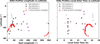 |
Fig. 2 Location on Venus of all the VeRa radio occultation soundings included in this study in terms of latitude−longitude (left panel) and latitude–local solar time (right panel). |
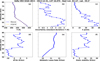 |
Fig. 3 Example of a temperature profile derived from VeRa radio occultation data for orbit ID 2811 (31 December 2013). (a) 1-km binned profile (dots) and the original profile (line). Binning removes the high-frequency components (see text). (b) Standard deviation of the temperature values that were averaged in each altitude bin, which is an indication of the uncertainty of the binned temperature values. (c) Number of values in each altitude bin. (d) Temperature gradient derived from the temperature profile. (e) Adiabatic lapse rate from Seiff et al. (1980). (f) Static stability, the temperature gradient minus the adiabatic lapse rate. |
2.3 VMC dataset
To perform the VMC - VeRA correlation, we performed two preparatory steps. First, we corrected for the movement of the atmosphere between the time of a VMC image and a VeRa radio occultation sounding due to winds. Second, we took into account the instrument calibration and observation geometry conditions to calculate a phase-corrected relative brightness.
2.3.1 Correction for wind advection
The time difference between VMC and VeRa observations,  -
-  , ranged from −11 to +1 hours. In this time interval, the cloud field is advected by atmospheric winds, which need to be taken into account when comparing the observations. We evaluated two possible approaches for this correction, using average wind fields and orbit-specific wind fields.
The most comprehensive analysis of mean zonal and meridional wind speeds for the cloud-top level using VMC-UV data is that reported by Khatuntsev et al. (2013). In Figure 10 of their paper, the average zonal and meridional winds are shown as a function of latitude between  and
and  in latitude. The strong zonal wind slowly increases from about
  at the equator to
  at a latitude of
  , and drops to
  at the pole. The meridional wind varies between
  near the equator and pole to about
  around
  in latitude. The spread in measured wind speeds can be seen in the figure:
  for the zonal wind and
  for the meridional wind. To access the wind speeds at any latitude, we used a linear parametrisation of the curves in latitude sections, making sure to stay within the error bars. For the zonal wind, we parametrised for latitude sections between
 ![Mathematical equation: \left[-90^{\circ},-50^{\circ}\right]](/articles/aa/full_html/2025/06/aa53905-25/aa53905-25-eq33.png) ,
, ![Mathematical equation: \left[-50^{\circ},-40^{\circ}\right],\left[-40^{\circ},-15^{\circ}\right]](/articles/aa/full_html/2025/06/aa53905-25/aa53905-25-eq34.png) , and latitudes
, and latitudes  . For the meridional wind, the latitude sections are
 ![Mathematical equation: \left[-90^{\circ},-75^{\circ}\right],\left[-75^{\circ},-50^{\circ}\right]](/articles/aa/full_html/2025/06/aa53905-25/aa53905-25-eq36.png) , and
, and ![Mathematical equation: \left[-50^{\circ},-20^{\circ}\right]](/articles/aa/full_html/2025/06/aa53905-25/aa53905-25-eq37.png) , and latitudes
, and latitudes  . Longitudinal or local solar time variations in the mean winds were not taken into account. We need to keep in mind that the values for the winds were derived from UV images, and hence they correspond to the altitude levels where the UV contrasts are present. As was discussed in the introduction, this is in the upper clouds at around
  in altitude (Crisp 1986; Sánchez-Lavega et al. 2008; Ignatiev et al. 2009; Lee et al. 2015b). The magnitude of the zonal and meridional wind changes with altitude: Sánchez-Lavega et al. (2017) show this variation measured by a variety of experiments between the surface and 70 km altitude for equatorial regions in their Fig. 1. To access this variation for other latitude regions, the cyclostrophic balance equation can be used, connecting the zonal winds with the temperature structure in the atmosphere (Fig. 9 in Sánchez-Lavega et al. (2017)). It is clear that the wind advection correction scheme we describe above is only valid within a restricted altitude range. We took this range to be approximately where the zonal wind velocities do not vary more than the uncertainties in the wind velocities we took into account as described above and restricted our further analysis to the
  altitude range. The meridional wind velocity variation with altitude is of the order of the spread quoted above (see Fig. 4 in Sánchez-Lavega et al. 2017).
The next step was to determine where the parcel of atmosphere sounded during a VeRa radio occultation at location ( ) had moved at the time a VMC image was acquired. We determined the co-ordinates (
 ) of this point from the time difference between the VMC image and the VeRa sounding and with the average wind speeds at the latitude
  , both in the zonal and meridional direction. We evaluated the uncertainty in (
 ), by doing the same calculation using the spread in the zonal (
 ) and meridional (
 ) winds. We obtained four additional co-ordinates that define a latitude-longitude box centred at (
 ). The size of this box is about
  in longitude and
  in latitude at the largest time difference of −11 h , and about one tenth of this at the smallest time difference of plus one hour.
The final step was to determine the average of the UV brightness within this box and take this as the VMC radiance for the sounding location for that image. The UV brightness of each pixel was calculated taking into account the incidence and phase angles of the observation, as is described in Section 2.3.2. The uncertainty was taken to be the standard deviation of the average of all the pixels within the latitude−longitude box.
The winds at any given time may deviate from their mean values. We evaluated whether when using wind speeds values obtained during a specific orbit a more accurate advection correction would be obtained, compared to using mission mean wind speeds. This was particularly possible for the data from the South Polar Dynamics Campaign, because VMC images were taken at regular (about 30 minute) intervals. Khatuntsev & Patsaeva (2025) provided wind vectors for 18 orbits from the South Polar Dynamics Campaign. We compared the centres of the latitude-longitude boxes derived in this way with the ones derived using mission average wind speed values, and we saw that they overlap within the uncertainties. In fact, the uncertainties in the positions when using orbit specific wind speed values were found to be higher. We therefore decided it would be more consistent to use the mission average values throughout our analysis.
In Fig. 4, we illustrate the result of the procedure with three images from orbit 2805 (25 December 2013) obtained, respectively,  , and 4 h before the VeRa sounding on that orbit. The latitude-longitude position of the VeRa sounded location is marked by a yellow star. The predicted location of the sounded air parcel (
 ) is marked as a red rectangle. It can be seen that the rectangle stays in roughly the same position with respect to cloud features in the time span between the VMC and VeRa observations, illustrating that the mean wind field captures the actual cloud motion accurately enough.
At this point, we note that the size of the latitude-longitude boxes is larger than the observed wavelengths of horizontal gravity waves. Piccialli et al. (2014) report maximum horizontal wavelengths of the order of 20 km . The minimum size of the boxes is of the order of 40 km , and the average value is of the order of 500 km ; hence, any effect due to horizontal gravity waves has been averaged out.
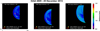 |
Fig. 4 Three images each taken two hours apart during ingress of orbit 2805 on 25 December 2013. The yellow star indicates the spot of the VeRa radio occultation that happens after |

2.3.2 Calculation of relative UV brightness
The VMC data used for this analysis are calibrated level 2 images obtained from the ESA Planetary Science Archive. The radiances measured in the images are a function of the incidence, emission, and phase angles of the observation. We applied a simple Lambert disc function as a photometric correction: the radiance divided by the cosine of the incidence angle. Lee et al. (2015a) demonstrate that this is sufficiently accurate (their Section 3.3) for viewing geometries where the phase angle does not exceed  and the incidence and emission angles are smaller than
  and
and  , respectively. We applied these same constraints for the images in our analysis.
In order to be able to compare radiances retrieved from images taken at different phase angles, we must take into account the scattering phase function. For this we built a phase curve, making use of all the 972 images from the 56 orbits in our analysis. We calculated the average radiance factor (see Lee et al. 2015a, Eq. (2)) for each image, taking all the pixels with the geometry conditions, as was described in the previous section. In Fig. 5a, we present the phase curve with this data, and the quadratic least square fit. We found that binning the results in phase angle bins of  width and taking the average in each bin results in an improved fit with a higher confidence level, as can be seen in Fig. 5b.
The grey area around the model curves in Fig. 5 is the uncertainty range. We derived this uncertainty range by randomly varying each of the bin-averaged radiance factors. To do this, we added a randomly drawn value from a Gaussian distribution to each bin-averaged radiance factor value. The average of this distribution is the bin-averaged radiance factor value. The standard deviation is the maximum of all the uncertainties on the individual radiance factors values in the bin and the uncertainty as assessed through equation 3.14 from Bevington & Robinson (2003). We did this exercise 1000 times and for each of these permutations we fitted a new model. We verified that the average radiance factor value of the models of the 1000 experiments for each phase angle bin is within  of the actual bin-averaged radiance factor. There are two ways to derive the uncertainty of the model radiance factor in each bin: either take the standard deviation of the 1000 experiments or take half the value of the maximum minus the minimum radiance ractors of the 1000 experiments. We compared both and decided to take the maximum of the two, which turns out to be the second option and is of the order of
  for each bin radiance factor.
As is presented in Section 2.3.1, we tracked the area of a VeRa sounding (latitude-longitude boxes) in the different images taken during the orbit. Given the scale of the latitude-longitude boxes and the uncertainties involved (Figs. 4a–c), the average radiance factors of latitude-longitude boxes measured from each of the images of one orbit should be similar. The observing geometry changes between images on an orbit. Hence, to compare between the images on one orbit, we used the model phase curve to normalise the average radiance factors for each image. We call these normalised radiance factors radiance factor ratios (RFRs). In Fig. 6, we present examples of RFR for the tracked VeRa areas on three different orbits, as a function of the time difference between the VMC image and the VeRa sounding (left column) and the phase angle (right column). The last row is for orbit 2805, the same as the example images shown in Fig. 4. The red line is the average RFR value over all the images of the orbit. The associated uncertainty (standard deviation) is represented by the red-shaded area. The green line and green-shaded area represent the median values and associated uncertainties (see Table A.1), respectively. The RFR values per image on one orbit are consistent, taking into account their uncertainties (blue error bars).
We recognise that our assumption of the phase function being applicable over all regions of the planet, including both bright and dark patches, ignores any possible localised changes in microphysical properties of the scattering particles or cloudtop altitudes. We note, however, that a higher-order phase function correction scheme would not be supported by the relatively sparse and noisy dataset we have here. An extensive analysis of how phase functions vary from dark to light regions on Venus, using the more sensitive  region of the phase function, may be found elsewhere; for example, in Petrova et al. (2015) and Shalygina et al. (2015).
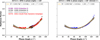 |
Fig. 5 Phase curve for all valid images of this study: (a) all images individually; (b) same as (a) but binned in bins of |

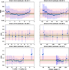 |
Fig. 6 Examples of the RFRs for sequences of images on a same orbit, derived from the radiance factors extracted from the latitude-longitude boxes of the wind-advected areas (Fig. 4) and applying the phase curve model (Fig. 5). We expect these values to be very similar throughout one orbit. The average and standard deviation is shown in red; the median and associated uncertainties in green. See also Table A.1. |
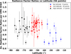 |
Fig. 7 Average UV RFRs of the VeRa sounding locations as a function of latitude of the VeRa sounding location. The different colours indicate the division we made to try minimise the effect of variation in the UV brightness with latitude when doing the statistical analysis. |
3 Analysis
The goal of our analysis is to investigate whether any correlation can be found between the temperature structure derived from VeRa observations of a small area on Venus and the UV brightness of that same area. As was discussed in the introduction, the UV contrasts are understood to originate in the upper clouds at an altitude of around  (Crisp 1986; Sánchez-Lavega et al. 2008; Ignatiev et al. 2009; Lee et al. 2015b), where about half of the solar UV energy is deposited. It would therefore be expected that any correlations would preferentially occur in this altitude range. The clouds are vertically extended with a scale height of several kilometres, and therefore the deposition of energy is expected to happen over a range of altitudes and not be sharply bound. We systematically explored this question by comparing the average (UV) RFR per orbit and the temperature derived from VeRa radio occultations, as well as RFR and the static stability in the region between 65 and 75 km in altitude.
It is well known that the temperature and upper cloud structure on Venus show variations with latitude. Not all of this variation has been explained, however (Lee et al. 2015b). Also, the overall UV brightness changes with latitude. In Fig. 7, we show the average RFRs derived from our selection of images (Table A.1) versus latitude.
From a more exhaustive analysis, it is known that the highest UV brightness is typically found at mid-latitudes ( through −
  ), and the darkest regions are found at low latitudes (Lee et al. 2015a). We can see this trend in Fig. 7. In Fig. 8, we present the VeRa temperatures at 65,67 , and 75 km altitude as a function of latitude from the 56 temperature profiles (Table A.1).
This latitudinal variation echoes what has previously been reported for the full VeRa dataset by Tellmann et al. (2009), as well as from IR sounding (Zasova et al. 2007): at higher altitudes, the poles are warmer than the equator compared to lower altitudes; around the cloud tops, there is a more equal situation. It is interesting to get an idea of the correlation between temperature and latitude without assuming any specific function.
A suitable way to evaluate this is to calculate the Spearman’s rank correlation coefficient. This coefficient is a measure of how monotonically correlated the data is by evaluating the linearity of the ranked version of the data. The Spearman’s rank correlation coefficient takes values between −1 and +1 : the closer to  , the stronger the (anti-)correlation, whereas values around zero mean there is no correlation. In Fig. 9, we present the Spearman’s rank correlation coefficient in blue as a function of altitude as derived from our data point (Figures 8a–c).
It can be seen that there is a strong correlation for altitudes of  , a strong anti-correlation for
  , and weak or no correlation for
  . From visual inspection of the examples in Fig. 8, a linear correlation seems to exist, though it is unclear why the correlation would be linear. The Pearson correlation coefficient is a measure of the degree of linearity: it is the covariance of the two variables divided by the product of their standard deviations. Note that the Spearman’s rank correlation coefficient is the Pearson correlation coefficient of the ranked data: while using the Pearson’s correlation we evaluate linear relationships, with the Spearman’s correlation we evaluate monotonic relationships, linear or not. We calculate and show this coefficient in red in Fig. 9. We used this to correct for the latitudinal variation, as is explained in the next section.
We decided to do our analysis in latitude bins in an effort to minimise latitudinal-variation effects. From Figs. 7 and 9, and from considering the cloud top altitude changes that affect the radiative balance (Lee et al. 2015b), we decided on three latitude bins: low latitudes between  and
and  (9 data points), mid latitudes between
  and
and  (30 data points), and high latitudes between
  and
and  (17 data points). These are indicated in Fig. 7 with vertical green lines.
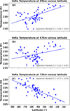 |
Fig. 8 Temperature derived from 56 VeRa soundings (Table A.1) as a function of latitude at 65,67 , and 75 km in altitude. There is a clear correlation at the lower and higher altitudes and no clear correlation in between. This is also clearly seen in Fig. 9, where the Spearman’s rank and Pearson correlation coefficients are shown as a function of altitude. The lines are the least square linear fits. |
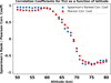 |
Fig. 9 Pearson correlation coefficient (red) and Spearman’s rank correlation coefficient (blue) for temperature as a function of latitude at altitudes between 50 and 80 km ; see also Fig. 8. At lower and higher altitudes, the correlation between temperature and latitude seems to be fairly well described with a line, the reason for which is not obvious. |
3.1 UV brightness versus temperature correlation
We calculated Spearman’s rank correlation coefficients for the RFR versus the VeRa temperature at altitude levels between 65 and 75 km in each of the three latitude bins. We estimated the uncertainties in the coefficients by running 1000 experiments, changing the RFR and temperature values by adding random values from a Gaussian distribution that is characterised by the average and standard deviation of each RFR and temperature values. The result is shown in the top right panel of Fig. 10 and an example of RFR versus VeRa temperature at an altitude of 67 km in Fig. 11. A negative Spearman’a rank correlation coefficient means that the UV brightness decreases as the temperature increases.
We also determined the corresponding one-sided p values and they are plotted in the bottom panels of Fig. 10. The p value is a measure of the probability that the observed correlation is due to chance. To evaluate the significance of a possible correlation, we chose a p-value limit of 0.02 , which corresponds to about  in a Gaussian distribution. For the RFR versus VeRa temperature correlations, the p value drops below 0.02 only at 67 km in altitude, where it reaches 0.009 . Hence, only at this altitude can the correlation not be considered to be due to chance.
As was mentioned above and as can be seen from Fig. 8 and Fig. 9, the temperatures show little variation with latitude in the  altitude range, but a stronger variation at other altitudes. The latitude-binning process does not fully account for the effect of these temperature variations. To address this we normalised the temperatures by dividing them to the least square linear fit of the temperature variation with latitude at each altitude. These fits are shown in Fig. 8. The evaluation of the Pearson correlation coefficient for the variation of the temperature with latitude seems to validate that a least square fitted line is a good option (Fig. 9). An example of RFR as a function of normalised temperature is shown for an altitude of 67 km in the right panel of Fig. 11. Normalising the temperatures to such a model for each altitude and performing the correlation analysis again results in a correlation plot shown in the right top panel of Fig. 10 As was expected, the structure and Spearman’s rank correlation coefficient values remain very similar in the
  altitude range, and only change somewhat in the
  altitude region. The corresponding p values show two altitudes at which they drop below 0.02, at 67 and 68 km in altitude, where the values are 0.01 and 0.011, respectively.
Despite our efforts to reduce the data as accurately and rigorously as possible, the data is rather noisy, which leads to quite some scatter. Yet we can identify some features we feel confident about. The most obvious is that there seems to be a stronger tendency for anti-correlation between the UV brightness and the temperature in the low and mid latitude bins in the  altitude range: in these regions UV-dark areas are a few degrees hotter than in UV-bright regions. This could be a direct consequence of solar UV-energy deposition in this altitude range and it is instructive to examine how this temperature difference compares with theoretical expectations. Crisp (1986, Figure 11) and Tomasko et al. (1985) present global mean heating rates for highand low-UV absorber cases, defined primarily from analysis of Pioneer Venus probe data, which have higher and lower heating rates, respectively. We can take these model extremes as proxies for the variation we observe in the UV RFR. In the
  altitude range, the difference between the global mean heating rates from the two models is of the order of
  (Earth)day. The heating rate at the sub-solar point can be estimated to be a factor of 4 higher than the global mean heating rate (area of sphere versus area of circle). If a UV-dark or UV-bright feature at the equator is sustained for 2 Earth days, the time it takes to move from dawn to dusk at these altitudes, then the average heating rate over the course of 12 h local solar time and changing solar incidence angle will be a factor of
  the sub-solar heating rate. This results in a total factor of about 5 (4 times 2 (Earth days) times
  ). Hence, the temperature difference between a high-UV absorber and low-UV-absorber calculated from the Crisp model heating rates will be of the order of
  . This is the calculated value at the equator, and would be correspondingly reduced by a factor of cosine(latitude) for other latitudes; if averaged over the latitude band of 0−40 degrees, the calculated temperature difference would be less by 10 percent or so, of the order of
  . In the left panel of Fig. 11, where the UV RFR versus temperature at 67 km altitude is shown, the blue points (low latitudes, showing anti-correlation, see Fig. 10) span a range of about 10 K , which is most certainly in the same ballpark as the model-estimated value. This agreement between observed values and model predictions is encouraging, particularly given that this is observed only in the low latitude region, where solar heating would be expected to be most significant, and because the altitude range where the heating is observed also corresponds to that in Crisp’s model.
3.2 UV brightness − static stability correlation
We also analysed any possible correlation between the UV brightness and the static stability. We followed a similar process to the analysis on the correlation with temperature presented in the previous section. The difference is that there is no variation in static stability with latitude in the 50 to 80 km altitude range, and hence no need to perform any normalisation correction. The Spearman’s rank correlation coefficient for the RFR versus static stability for each altitude level is shown in the top panel of Fig. 12 and the corresponding p values in the bottom panel. This result shows more scatter than the ones for the VeRa temperature correlation. The corresponding p values never drop below the 0.02 limit.
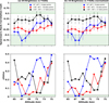 |
Fig. 10 Spearman’s rank correlation coefficients for UV RFR as a function of temperature (left column) and normalised temperature (right column), at levels between 65 and 75 km in altitude for three latitude bins. Normalisation of the temperature was done to compensate for changes in the temperature with latitude that were not fully accounted for by dividing the data into three latitude bins. The largest effect is at the lower and higher altitudes, where the change of temperature with latitude is strongest (Figs. 8,9,11). The green areas in the figure indicate moderate to strong correlation. The corresponding one-sided p value for each of the correlations is shown in the bottom panels. We chose a limit of |


4 Conclusion
We have analysed the possibility of correlation between the UV brightness and the temperature structure in the atmosphere using unique data from Venus Express. On the one hand, these data are measurements of the temperature structure from radio occultation data (VeRa experiment) in very small areas on Venus; on the other hand, they are UV-images of the same spot up to 11 hours before and a few hours after the radio occultation experiment (VMC instrument). This type of analysis has not been presented before, as no such data exist from earlier missions.
We have reduced the data, taking into account all sources of uncertainty. Though the final result is still rather noisy, we find that there is an anti-correlation between the atmospheric temperature around the 67 km altitude range and the UV brightness for the low latitude region (latitudes lower than  ), with a one-sided p value smaller than 0.02 ; hence, it is highly unlikely that this is due to chance. From theoretical radiative forcing studies and in situ descent probe measurements of the net radiative flux, it is known that the solar UV-energy is deposited in this altitude range. The temperature difference between UV-dark and UV-bright regions, and its altitude dependence, is similar to that expected from increased solar heat absorption in UVdark regions, approximately matching expectations. Our result also provides the possible vertical location of the solar energy deposition in the
  altitude range, implying that the UV-to-blue-absorber may exist in this vertical layer (Tomasko et al. 1985; Crisp 1986; Lee et al. 2015b, 2021) rather than being well mixed through the upper haze layer (Molaverdikhani et al. 2012). The assumption of a well-mixed unknown UV-to-blue-absorber above the cloud-top level was also used in the analysis of other spectral data (Pérez-Hoyos et al. 2018; Marcq et al. 2020), while its impacts on solar heating have not yet been quantified. Such a vertical distribution may change over time Lee et al. (2015a), but since there is no similar dataset for other earlier missions a possible temporal variation in heating altitudes cannot be done at this moment.
The present analysis has not shown any correlation between UV brightness and stability. A correlation between UV brightness and stability could indicate that convective overturning is bringing UV-to-blue-absorber to the cloud tops; conversely, an anti-correlation could indicate that convective overturning is bringing cloud-forming volatiles to the cloud tops. A further study may be conducted targeting static stability, using very fine-vertical-resolution data of radio occultation measurements similar to what Imamura et al. (2018) achieved.
The present analysis has shown a hint of a correlation between the UV brightness and the temperature structure in the atmosphere from Venus Express data, though it is not a very robust conclusion. However, the techniques used here could be applied to larger datasets from future missions.
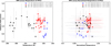 |
Fig. 11 RFR versus temperature (left) and normalised temperature (right) at 67 km altitude. Normalisation was done relative to a linear least square fit to the temperature as a function of latitude at each level between 50 and 80 km altitude. See Figs. 8 and 9. |
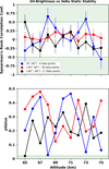 |
Fig. 12 Spearman’s rank correlation coefficient for RFR as a function of static stability in the |


Acknowledgments
The authors thank the anonymous reviewer and the A&A editor Emmanuel Lellouch for constructive comments and feedback that improved the quality of the presented work. MRS thanks Emmanuel Marcq for sharing VIRTIS - SPICAV results and constructive discussion. YJL was supported by the Institute for Basic Science (IBS-R035-C1). A full note book and all the (Python) scripts created and used for this study can be found at the open Codeberg repository: https://codeberg.org/PleaseStateTheNatureOfYourInquiry/VenusResearchWorkBook. See also link to the digital Venus Research Workbook at the end of the README section, as well as the link to the images and temperature profiles used in this analysis. The resulting wind tracking vectors for ultraviolet (365 nm) images obtained by the Venus Monitoring Camera (VMC) on board Venus Express for 18 orbits from the South Polar Dynamics Campaign (orbits numbers 2778−2811) are available in Mendeley Data (Khatuntsev & Patsaeva 2025).
Appendix A Data table
Venus Express orbits with VeRa radio occultation soundings
References
- Akiba, M., Taguchi, M., Fukuhara, T., et al. 2021, J. Geophys. Res. (Planets), 126, e06808 [NASA ADS] [Google Scholar]
- Barstow, J. K., Tsang, C. C. C., Wilson, C. F., et al. 2012, Icarus, 217, 542 [NASA ADS] [CrossRef] [Google Scholar]
- Bevington, P. R., & Robinson, D. K. 2003, Data reduction and error analysis for the physical sciences (Boston, MA: McGraw-Hill) [Google Scholar]
- Coblentz, W., & Lampland, C. 1925, J. Franklin Inst., 119, 785 [Google Scholar]
- Cottini, V., Ignatiev, N. I., Piccioni, G., & Drossart, P. 2015, Planet. Space Sci., 113, 219 [Google Scholar]
- Crisp, D. 1986, Icarus, 67, 484 [NASA ADS] [CrossRef] [Google Scholar]
- Ekonomov, A. P., Moroz, V. I., Moshkin, B. E., et al. 1984, Nature, 307, 345 [Google Scholar]
- Esposito, L. W., Bertaux, J. L., Krasnopolsky, V., Moroz, V. I., & Zasova, L. V. 1997, in Venus II: Geology, Geophysics, Atmosphere, and Solar Wind Environment, eds. S. W. Bougher, D. M. Hunten, & R. J. Phillips, 415 [Google Scholar]
- Frandsen, B. N., Wennberg, P. O., & Kjaergaard, H. G. 2016, Geophys. Res. Lett., 43, 11146 [Google Scholar]
- Herrmann, M., Häusler, B., Pätzold, M., Tellmann, S., & Oschlisniok, J. 2014, in European Planetary Science Congress, 9, EPSC2014–125 [Google Scholar]
- Ignatiev, N. I., Titov, D. V., Piccioni, G., et al. 2009, J. Geophys. Res. (Planets), 114, E00B43 [CrossRef] [Google Scholar]
- Imamura, T., Miyamoto, M., Ando, H., et al. 2018, J. Geophys. Res. (Planets), 123, 2151 [Google Scholar]
- Khatuntsev, I. V., & Patsaeva, M. 2025, Dataset on Mendeley, https://doi.org/10.17632/25447wz6gg.1 [Google Scholar]
- Khatuntsev, I. V., Patsaeva, M. V., Titov, D. V., et al. 2013, Icarus, 226, 140 [NASA ADS] [CrossRef] [Google Scholar]
- Kouyama, T., Imamura, T., Taguchi, M., et al. 2017, Geophys. Res. Lett., 44, 12098 [Google Scholar]
- Lee, Y. J., García Muñoz, A., Imamura, T., et al. 2020, Nat. Commun., 11, 5720 [NASA ADS] [CrossRef] [Google Scholar]
- Lee, Y. J., García Muñoz, A., Yamazaki, A., et al. 2021, Geophys. Res. Lett., 48, e90577 [NASA ADS] [Google Scholar]
- Lee, Y. J., Imamura, T., Schröder, S. E., & Marcq, E. 2015a, Icarus, 253, 1 [Google Scholar]
- Lee, Y. J., Titov, D. V., Ignatiev, N. I., et al. 2015b, Planet. Space Sci., 113, 298 [Google Scholar]
- Lee, Y. J., Jessup, K.-L., Perez-Hoyos, S., et al. 2019, AJ, 158, 126 [NASA ADS] [CrossRef] [Google Scholar]
- Marcq, E., Baggio, L., Lefèvre, F., et al. 2019, Icarus, 319, 491 [NASA ADS] [CrossRef] [Google Scholar]
- Marcq, E., Lea Jessup, K., Baggio, L., et al. 2020, Icarus, 335, 113368 [NASA ADS] [CrossRef] [Google Scholar]
- Markiewicz, W. J., Titov, D. V., Ignatiev, N., et al. 2007, Planet. Space Sci., 55, 1701 [Google Scholar]
- Molaverdikhani, K., McGouldrick, K., & Esposito, L. W. 2012, Icarus, 217, 648 [Google Scholar]
- Patsaeva, M. V., Khatuntsev, I. V., Patsaev, D. V., et al. 2015, Planet. Space Sci., 113, 100 [Google Scholar]
- Pätzold, M., Häusler, B., Bird, M. K., et al. 2007, Nature, 450, 657 [CrossRef] [Google Scholar]
- Pérez-Hoyos, S., Sánchez-Lavega, A., García-Muñoz, A., et al. 2018, J. Geophys. Res. (Planets), 123, 145 [Google Scholar]
- Petrova, E. V., Shalygina, O. S., & Markiewicz, W. J. 2015, Icarus, 260, 190 [Google Scholar]
- Piccialli, A., Titov, D. V., Sanchez-Lavega, A., et al. 2014, Icarus, 227, 94 [NASA ADS] [CrossRef] [Google Scholar]
- Pollack, J. B., Toon, O. B., Whitten, R. C., et al. 1980, J. Geophys. Res., 85, 8141 [Google Scholar]
- Ross, F. E. 1928, ApJ, 68, 57 [Google Scholar]
- Sánchez-Lavega, A., Hueso, R., Piccioni, G., et al. 2008, Geophys. Res. Lett., 35, L13204 [Google Scholar]
- Sánchez-Lavega, A., Lebonnois, S., Imamura, T., Read, P., & Luz, D. 2017, Space Sci. Rev., 212, 1541 [CrossRef] [Google Scholar]
- Seiff, A., Kirk, D. B., Young, R. E., et al. 1980, J. Geophys. Res., 85, 7903 [CrossRef] [Google Scholar]
- Shalygina, O. S., Petrova, E. V., Markiewicz, W. J., Ignatiev, N. I., & Shalygin, E. V. 2015, Planet. Space Sci., 113, 135 [Google Scholar]
- Svedhem, H., Titov, D. V., McCoy, D., et al. 2007, Planet. Space Sci., 55, 1636 [Google Scholar]
- Tellmann, S., Pätzold, M., Häusler, B., Bird, M. K., & Tyler, G. L. 2009, J. Geophys. Res. (Planets), 114, E00B36 [Google Scholar]
- Tellmann, S., Häusler, B., Hinson, D. P., et al. 2012, Icarus, 221, 471 [Google Scholar]
- Titov, D. V., Taylor, F. W., Svedhem, H., et al. 2008, Nature, 456, 620 [Google Scholar]
- Tomasko, M. G., Doose, L. R., Smith, P. H., & Odell, A. P. 1980, J. Geophys. Res., 85, 8167 [Google Scholar]
- Tomasko, M. G., Doose, L. R., & Smith, P. H. 1985, Adv. Space Res., 5, 71 [Google Scholar]
- Toon, O. B., Turco, R. P., & Pollack, J. B. 1982, Icarus, 51, 358 [Google Scholar]
- Wright, W. H. 1927, PASP, 39, 220 [Google Scholar]
- Zasova, L. V., Ignatiev, N., Khatuntsev, I., & Linkin, V. 2007, Planet. Space Sci., 55, 1712 [Google Scholar]
All Tables
All Figures
|
Fig. 1 Schematic of Venus Express orbit around Venus with VMC imaging happening on ingress and egress (blue dots) and VeRa radio occultation shortly after periapsis (red dot). |
| In the text | |
|
Fig. 2 Location on Venus of all the VeRa radio occultation soundings included in this study in terms of latitude−longitude (left panel) and latitude–local solar time (right panel). |
| In the text | |
|
Fig. 3 Example of a temperature profile derived from VeRa radio occultation data for orbit ID 2811 (31 December 2013). (a) 1-km binned profile (dots) and the original profile (line). Binning removes the high-frequency components (see text). (b) Standard deviation of the temperature values that were averaged in each altitude bin, which is an indication of the uncertainty of the binned temperature values. (c) Number of values in each altitude bin. (d) Temperature gradient derived from the temperature profile. (e) Adiabatic lapse rate from Seiff et al. (1980). (f) Static stability, the temperature gradient minus the adiabatic lapse rate. |
| In the text | |
|
Fig. 4 Three images each taken two hours apart during ingress of orbit 2805 on 25 December 2013. The yellow star indicates the spot of the VeRa radio occultation that happens after |
| In the text | |
|
Fig. 5 Phase curve for all valid images of this study: (a) all images individually; (b) same as (a) but binned in bins of |
| In the text | |
|
Fig. 6 Examples of the RFRs for sequences of images on a same orbit, derived from the radiance factors extracted from the latitude-longitude boxes of the wind-advected areas (Fig. 4) and applying the phase curve model (Fig. 5). We expect these values to be very similar throughout one orbit. The average and standard deviation is shown in red; the median and associated uncertainties in green. See also Table A.1. |
| In the text | |
|
Fig. 7 Average UV RFRs of the VeRa sounding locations as a function of latitude of the VeRa sounding location. The different colours indicate the division we made to try minimise the effect of variation in the UV brightness with latitude when doing the statistical analysis. |
| In the text | |
|
Fig. 8 Temperature derived from 56 VeRa soundings (Table A.1) as a function of latitude at 65,67 , and 75 km in altitude. There is a clear correlation at the lower and higher altitudes and no clear correlation in between. This is also clearly seen in Fig. 9, where the Spearman’s rank and Pearson correlation coefficients are shown as a function of altitude. The lines are the least square linear fits. |
| In the text | |
|
Fig. 9 Pearson correlation coefficient (red) and Spearman’s rank correlation coefficient (blue) for temperature as a function of latitude at altitudes between 50 and 80 km ; see also Fig. 8. At lower and higher altitudes, the correlation between temperature and latitude seems to be fairly well described with a line, the reason for which is not obvious. |
| In the text | |
|
Fig. 10 Spearman’s rank correlation coefficients for UV RFR as a function of temperature (left column) and normalised temperature (right column), at levels between 65 and 75 km in altitude for three latitude bins. Normalisation of the temperature was done to compensate for changes in the temperature with latitude that were not fully accounted for by dividing the data into three latitude bins. The largest effect is at the lower and higher altitudes, where the change of temperature with latitude is strongest (Figs. 8,9,11). The green areas in the figure indicate moderate to strong correlation. The corresponding one-sided p value for each of the correlations is shown in the bottom panels. We chose a limit of |
| In the text | |
|
Fig. 11 RFR versus temperature (left) and normalised temperature (right) at 67 km altitude. Normalisation was done relative to a linear least square fit to the temperature as a function of latitude at each level between 50 and 80 km altitude. See Figs. 8 and 9. |
| In the text | |
|
Fig. 12 Spearman’s rank correlation coefficient for RFR as a function of static stability in the |
| In the text | |
Current usage metrics show cumulative count of Article Views (full-text article views including HTML views, PDF and ePub downloads, according to the available data) and Abstracts Views on Vision4Press platform.
Data correspond to usage on the plateform after 2015. The current usage metrics is available 48-96 hours after online publication and is updated daily on week days.
Initial download of the metrics may take a while.