| Issue |
A&A
Volume 679, November 2023
|
|
|---|---|---|
| Article Number | A155 | |
| Number of page(s) | 10 | |
| Section | Planets and planetary systems | |
| DOI | https://doi.org/10.1051/0004-6361/202347714 | |
| Published online | 30 November 2023 | |
Determination of the eddy diffusion in the Venusian clouds from VeRa sulfuric acid observations
1
College of Meteorology and Oceanography, National University of Defense Technology,
Changsha, PR China
e-mail: This email address is being protected from spambots. You need JavaScript enabled to view it.
; This email address is being protected from spambots. You need JavaScript enabled to view it.
2
National Space Institute, Technical University of Denmark,
Lyngby, Denmark
3
Planetary Environmental and Astrobiological Research Laboratory (PEARL), School of Atmospheric Sciences, Sun Yat-sen University,
Zhuhai, PR China
Received:
12
August
2023
Accepted:
22
September
2023
Abstract
Context. The vertical eddy diffusion coefficient (Kzz) characterizing the efficiency of vertical atmospheric mixing is essential for 1D planetary atmospheric modeling, but poorly constrained in the Venusian clouds, where our ability to observe tracer gases is limited. The Venusian clouds are mainly composed of H2SO4, which has significant mass cycles in this region. A critical process herein is that the H2SO4 vapor abundance in the middle and lower clouds of Venus is regulated by both condensation and eddy diffusion processes.
Aims. This study is devoted to proposing a novel approach to estimating the Venusian cloud Kzz, examining the variability of the cloud Kzz in both equatorial and polar regions, and evaluating the derived Kzz through the implementation of a 1D photochemical model.
Methods. The H2SO4 vapor data used in this study were obtained from observations conducted by Venus Express. A novel approach that relies on the premise that both eddy diffusion and condensation regulate the abundance of H2SO4 vapor was then applied to estimate the Venusian cloud Kzz. The global mean Kzz and its latitudinal variation were discussed. A 1D photochemistry-diffusion model was applied to evaluate the estimations.
Results. Our calculations indicate that the global mean Kzz reaches 5 × 108 cm2 s−1 in the lower clouds, which is an order of magnitude larger than several observation-based estimations and model results. It rapidly decreases as the altitude increases above 54 km. Equatorial Kzz is three times as large as polar Kzz at 48 km, while polar Kzz reaches its peak below 46.5 km, where equatorial Kzz rapidly decreases as the altitude decreases.
Conclusions. We provide an estimate of the Venusian cloud Kzz based on H2SO4 vapor observations. Significant latitudinal variations exist in the Venusian cloud Kzz.
Key words: planets and satellites: individual: Venus / planets and satellites: atmospheres
© The Authors 2023
 Open Access article, published by EDP Sciences, under the terms of the Creative Commons Attribution License (https://creativecommons.org/licenses/by/4.0), which permits unrestricted use, distribution, and reproduction in any medium, provided the original work is properly cited.
This article is published in open access under the Subscribe to Open model. This email address is being protected from spambots. You need JavaScript enabled to view it. to support open access publication.
1 Introduction
The vertical eddy diffusion coefficient (Kzz) is a parameter characterizing the efficiency of vertical atmospheric mixing, incorporating turbulence, convection, and wave-induced processes. These eddy motions could occur across a wide variety of spatial scales, making them challenging to trace directly, and thus poorly constrained. Nevertheless, Kzz is widely used in various planetary atmospheric studies, especially in 1D photochemical and cloud models that are unable to resolve 3D eddies.
Determining the planetary atmospheric Kzz typically relies on analysis of the vertical distributions of atmospheric species. Inert gases or species with low chemical activity, such as He and CO, are commonly selected as trace species. By tracking the vertical eddy velocities of these species, atmospheric Kzz has been estimated on several planets (von Zahn et al. 1980; Mahieux et al. 2021; Swenson et al. 2019; Yoshida et al. 2022). However, Venus, covered globally by a thick layer of sulfuric acid clouds, poses challenges due to significant radiation absorption and scattering, restricting the detection of typical tracers in this region. Consequently, our knowledge of Venusian cloud Kzz remains limited. A recent model study has proposed that Kzz governs the H2SO4 cycle in the middle and lower clouds, leading to the mass accumulation in these regions (Dai et al. 2022b). Observations (Ando et al. 2020a; Hinson & Jenkins 1995; Imamura et al. 2017) and models (Ando et al. 2020b, 2022) have indicated a region of low static stability in the Venusian clouds, suggesting the presence of a convection layer. Notably, Ando et al. (2015) report significant latitudinal variability in the static stability distribution. Given the role of the Venusian clouds in regulating the global radiative transfer and subsequent climate change (Esposito et al. 1983; Titov et al. 2018; Turbet et al. 2021), a comprehensive understanding of Kzz in the clouds is crucial.
Due to the scarcity of observational constraints on the cloud Kzz, a variety of Kzz profiles have been used in the literature (see Table 1). Based on the in situ wind speed observations of Vega balloons (Sagdeev et al. 1986), the Kzz at 54 km has been estimated at 107 cm2 s−1 (Blamont et al. 1986). Pioneer Venus radio scintillation measurements estimated the Kzz to be 2 × 103 cm2 s−1 at 45 km (Woo et al. 1982) and 4 × 104 cm2 s−1 at 60 km (Woo & Ishimaru 1981).
Most microphysical models empirically assumed the cloud Kzz. The Kzz has been estimated to be 104−106 cm2 s−1 in 50–56 km (Imamura & Hashimoto 2001; Gao et al. 2014) and 104−107 cm2 s−1 in 50–57 km (McGouldrick & Toon 2007). This indicates an enhancement of the convection in the lower and middle clouds, corresponding to the observed strong wind shears near the cloud base (Kerzhanovich & Marov 1983) and cloud top (Imamura et al. 2020). The latest 3D large-eddy simulation indicates an enhancement of Kzz from 6 × 10⁴ to 1 × 108 cm2 s−1, extending from 48 to 56 km (Lefèvre et al. 2022). Besides, empirical cloud Kzz profiles have commonly been employed in 1D photochemical models. Krasnopolsky (2012) assumed a constant Kzz of 1 × 104 cm2 s−1 below 55 km. Zhang et al. (2012a) and Shao et al. (2020) estimate the Kzz in 58–80 km to be 4–5×104 cm2 s−1 by linearly interpolating the observed values at 60 and 80 km. Bierson & Zhang (2020) examined a weak cloud Kzz in the 45–65 km region, assuming a constant value of 1 × 103 cm2 s−1 to interpret the SO2 depletion in the clouds. However, this weak cloud Kzz contradicts the low static stabilities observed by Venus Express (Ando et al. 2015) and Akatsuki (Imamura et al. 2017).
This study aims to address three main objectives: (a) proposing a novel approach to estimating the Venusian cloud Kzz by utilizing the H2SO4 vapor mixing ratio profiles from Venus Express measurements; (b) examining the variability of the cloud Kzz in both the equatorial and polar regions; and (c) evaluating the derived Kzz through the implementation of a 1D photochemical model. The details regarding the data and methodology employed in this study are presented in Sect. 2. The results obtained are presented in Sect. 3. Furthermore, the evaluation through the 1D photochemistry-diffusion simulation is discussed in Sect. 4. Finally, we conclude the study in Sect. 5.
Venusian cloud Kzz in literature.
2 Data and method
2.1 Data
The H2SO4 vapor profiles used in estimating the Kzz were obtained from observations conducted by Venus Express (Oschlisniok et al. 2021). The presence of globally distributed thick clouds and the unknown UV absorber on Venus result in significant opacity in the visible and ultraviolet wavelengths, obstructing the visibility of most cloud features (Limaye et al. 2018; Titov et al. 2018). However, H2SO4 vapor has been proposed to be a strong absorber of radio waves (Steffes & Eshleman 1982), allowing its transmission through the clouds. Oschlisniok et al. (2021) derived over 800 H2SO4 vapor abundance profiles in the cloud regions using dual-frequency (X/S-band) radio science open loop data from the radio occultation measurements (VeRa) onboard the Venus Express, collected between 2006 and 2014. The derived distributions of H2SO4 vapor abundance, temperature, and pressure are presented in Figs. 1a–c. In the polar regions, H2SO4 vapor exhibits a concentration within the altitude range of 40–44 km, while at the equator this peak shifts to 45–48 km. The temperature distribution exhibits an arch-shaped pattern, while the pressure shows minimal latitudinal variations. We note that the presented H2SO4 vapor measurements have removed the SO2 absorption by using an estimated SO2 distribution, according to Oschlisniok et al. (2021). Its uncertainty is discussed in Sect. 5.
2.2 Method of Kzz estimation
In this study, the equilibrium between the vertical transports and the other sources and sinks of H2SO4 vapor serves as the foundation for the calculation of Kzz. Both observations (Imamura et al. 2017; Oschlisniok et al. 2021) and models (Dai et al. 2022b,a; Krasnopolsky 2015) indicate a rapid decrease in the H2SO4 vapor mixing ratio above the cloud base. The vertical diffusion flux of H2SO4 vapor becomes negligible above 55 km (Gao et al. 2014; Imamura & Hashimoto 2001). Thus, we chose 55 km as the upper boundary of our domain and assumed that the diffusion flux of H2SO4 vapor was zero at this altitude. The lower boundary of our domain is at the cloud base altitudes ranging from 43 to 47 km, varying with latitudes. The definition of the cloud base is described later.
Ahead of handling, the H2SO4 data was vertically smoothed by a Savitzky-Golay Filter (Savitzky & Golay 1964; Schafer 2011, impulse response length L = 11, polynomial order ω = 1), for the purpose of decreasing the influences of statistical fluctuation and the convergence or divergence of horizontal H2SO4 vapor flow. In our domain, the H2SO4 vapor mixing ratio could be simultaneously influenced by diffusion, condensation, evaporation, and chemistry. The differential diffusion flux versus altitude is defined as
 (1)
(1)
where Φ = vns (v is the diffusion velocity and ns the number density of H2SO4 vapor), z represents the altitude, and the terms at the right-hand side of the equation represent the rates of evaporation, condensation, chemical production, and loss, respectively. The net condensation or evaporation rate of H2SO4 vapor is written as (Seinfeld & Pandis 2016, p. 538–540)
![Mathematical equation: ${S_{\,{\rm{net}}}} = {S_{\,{\rm{evap}}}} - {S_{\,{\rm{cond}}}} = - \sum\nolimits_i {\left[ {{{2\pi \Theta _i^{\rm{p}}D} \over {kT}}{f_i}\left( {P - {P^{{\rm{svp}}}}{{\rm{e}}^{{{4\sigma M} \over {RT\rho \Theta _i^{\rm{p}}}}}}} \right)n_i^{\rm{p}}} \right],} $](/articles/aa/full_html/2023/11/aa47714-23/aa47714-23-eq2.png) (2)
(2)
where D is the molecular diffusion coefficient, k the Boltzmann constant, T the atmospheric temperature, P the pressure of H2SO4 vapor, and Psvp the saturation vapor pressure. The factor of Psvp represents the Kelvin Effect, where σ=71.11 erg cm−2 is the surface tension of sulfuric acid (Myhre et al. 1998), R is the gas constant, ρ = 1.8 g cm−3 is the mass density of the droplets. The distributions of particle diameter and number density are adopted from the cloud particle size spectrometer (LCPS) onboard the Pioneer Venus probes (Knollenberg & Hunten 1980), which cover several latitudes and are considered to be global mean distributions. We divided the observed diameters (ranging from 0.01 to 15 µm) into 32 bins (in log scale), counted as i.  and
and  represent the characteristic diameter and number density of bin i, respectively. D was calculated following Hamill et al. (1977):
 (3)
(3)
where Na is the Avogadro constant, M = 98 g mol−1 is the molecular weight of H2SO4, and λ is the mean free path of H2SO4 molecule, written as (Hamill et al. 1977)
![Mathematical equation: $\lambda = {\left[ {\pi {n_{{\rm{atm}}}}{{\left( {{{{d_{\rm{s}}} + {d_{{\rm{atm}}}}} \over 2}} \right)}^2}{{\left( {{{{M_{{\rm{atm}}}}} \over {M + {M_{{\rm{atm}}}}}}} \right)}^{{1 \over 2}}}} \right]^{ - 1}},$](/articles/aa/full_html/2023/11/aa47714-23/aa47714-23-eq6.png) (4)
(4)
where natm is the total atmospheric number density, ds = 4.4 × 10⁻⁸ cm (Hanson & Eisele 2000) and datm = 3.3 × 10⁻⁸ cm (Mehio et al. 2014) represent the molecular diameters of H2SO4 and the atmospheric major component (CO2), respectively, and Matm = 44 g mol−1 is the molecular weight of CO2. The flux-matching factor, fi, is adopted from Zhang et al. (2012b):
 (5)
(5)
where α = 1 is the accommodation coefficient (Seinfeld & Pandis 2016, p. 500–502).
The Psvp (in the unit of bar) depends on the atmospheric temperature and the droplet acidity, measured by
 (6)
(6)
where µ − µ0 is the difference in the chemical potential of H2SO4 between the solution and the pure condensate, adopted from the experimental data (Zeleznik 1991). The previously estimated cloud acidities from the observations have large uncertainties for either assuming a constant acidity throughout the clouds or that the observed spectrum was linearly interpolated among three acidity data points from experimental data (Arney et al. 2014; Palmer & Williams 1975), which showed a strong nonlinear dependence of the imaginary index of refraction on the cloud acidity (Barstow et al. 2012). Therefore, we adopted an acidity profile that reduces from 98% at the cloud base to 85% at 55 km, based on recent model results (Dai et al. 2022b; Krasnopolsky 2015; Stolzenbach et al. 2023).  is the SVP above the surface of pure H2SO4 condensate, adopted from the parameterization of 98% weight percentage H2SO4 (Kulmala & Laaksonen 1990):
![Mathematical equation: $\eqalign{ & \ln {P^{{\rm{svp}}}}{\rm{ (bar) }} = 16.259 - {{10156} \over {{T_0}}} \cr & \,\,\,\,\,\,\,\,\,\,\,\,\,\,\,\,\,\,\,\,\,\,\,\,\,\,\,\,\,\,\,\, + 10156\left[ { - {1 \over T} + {1 \over {{T_0}}} + {{0.38} \over {{T_{\rm{c}}} - {T_0}}}} \right. \cr & \left. {\,\,\,\,\,\,\,\,\,\,\,\,\,\,\,\,\,\,\,\,\,\,\,\,\,\,\,\,\,\,\,\,\, \times \left( {1 + \ln {{{T_0}} \over T} - {{{T_0}} \over T}} \right)} \right], \cr} $](/articles/aa/full_html/2023/11/aa47714-23/aa47714-23-eq10.png) (7)
(7)
where T0=360 K is a reference temperature and Tc=905 K is the critical temperature.
Three illustrative cases of the H2SO4 vapor mixing ratio and saturation vapor mixing ratio profiles in different latitudes are presented in Figs. 2a,d,g. The lowest intersections of the H2SO4 vapor mixing ratios and the saturation profiles occur at 47, 47, and 43.5 km, respectively, indicating the onset of condensation. These layers are defined as the cloud base in this study. Above the cloud base, the mixing ratios increase slightly to the peaks and then generally decrease as the altitude increases, with the presence of some fluctuations. The H2SO4 vapor mixing ratios are higher than the saturation lines at most altitudes except that an undersaturation region appears near 51 km in the polar case, attributed to the horizontal transport of H2SO4 vapor or a statistical fluctuation in the data. Additionally, Fig. 2b,e,h display the corresponding profiles of H2SO4 condensation or evaporation rates. These rates reach 1011−1012 cm−3 s−1 in the middle and lower clouds. Here we note that such high rates might lead to latent heat exchange, contributing to local temperature variation. However, since the temperature data we used was adopted from direct observations, and Kzz was calculated by vertical transport rather than static stability, the latent heat is not what this study needs to focus on. Chemical models (Bierson & Zhang 2020; Krasnopolsky 2007, 2012) suggest that the net production or thermal-decomposition rates of H2SO4 vapor in this region are lower than 1 × 105 cm−3 s−1. Therefore, the chemical processes were neglected in our investigation of Kzz in the middle and lower clouds of Venus. That is, Sprod-Sloss ≈ 0 cm−3 s−1. Then, the H2SO4 vapor flux at z altitude could be calculated by
 (8)
(8)
Subsequently, the diffusion velocity of H2SO4 vapor was calculated by:
 (9)
(9)
We note that this is the total diffusion velocity, that is, the combination of eddy diffusion and molecular diffusion. The total diffusion flux could be described as
![Mathematical equation: ${\rm{\Phi }} = - D{n_{\rm{s}}}\left( {{1 \over {{H_{\rm{s}}}}} + {{{\rm{d}}T} \over {T{\rm{d}}z}} + {{{\rm{d}}{n_{\rm{s}}}} \over {{n_{\rm{s}}}{\rm{d}}z}}} \right) - {K_{zz}}{n_{{\rm{atm}}}}\left[ {{{\rm{d}} \over {{\rm{d}}z}}\left( {{{{n_{\rm{s}}}} \over {{n_{{\rm{atm}}}}}}} \right)} \right],$](/articles/aa/full_html/2023/11/aa47714-23/aa47714-23-eq13.png) (10)
(10)
where Hs = kT/msg is the scale height of H2SO4 vapor, ms is the molecular weight of H2SO4, and g = 870 cm s−2 is the Venusian gravity acceleration. The general expression for the molecular and eddy diffusion velocities of H2SO4 vapor are
 (11)
(11)
 (12)
(12)
The eddy diffusion coefficient could be derived by
![Mathematical equation: ${K_{zz}} = - {{{v_{{\rm{eddy}}}}{n_{\rm{s}}}} \over {{n_{{\rm{atm}}}}\left[ {{{\rm{d}} \over {{\rm{d}}z}}\left( {{{{n_{\rm{s}}}} \over {{n_{{\rm{atm}}}}}}} \right)} \right]}}.$](/articles/aa/full_html/2023/11/aa47714-23/aa47714-23-eq16.png) (13)
(13)
The derived Kzz distributions in the specific scenarios are presented in Figs. 2c,f,i. In the lower cloud regions, the values reach magnitudes of 1 × 108 cm2 s−1. We note that occasional negative values occur at certain altitudes, especially near the top boundary. The H2SO4 data near the top boundary is occasionally negative due to its low abundance. This results in negative Kzz in this region. The effect of this issue could rapidly decrease with decreasing altitude since the low condensation or evaporation rate contributes less to its column integration. Besides, parameterizing the complicated 3D transport of atmosphere by 1D diffusion needs a great simplification, which might overlook some potential effects such as horizontal transport. The same negative Kzz has been indicated by Zhang & Showman (2018) to be the result of the non-diffusive effects regulating the atmosphere. 1D model studies (Dai et al. 2022b; Gao et al. 2014) proposed that H2SO4 vapor diffuses upward in the cloud layer to contain the formation of the thick clouds. However, the effects of statistical fluctuation and horizontal convergence or divergence, which are carried by H2SO4 vapor data and not completely removed by the smooth process, increase the local H2SO4 vapor abundance and possibly lead to a downward flux. Then, negative Kzz could also appear in these regions to correct the direction of the vapor flux. Since these issues are not able to be included in the 1D studies and could be diluted by horizontal averages, we removed these data points.
 |
Fig. 1 VeRa observations (Oschlisniok et al. 2021). The panels show (a) the H2SO4 vapor volume mixing ratio, (b) temperature, and (c) pressure, respectively. We note that these observations are divided into 36 latitudinal bins with a resolution of 5 degrees. The lack of measurements is caused by the orbit geometry of Venus Express. |
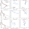 |
Fig. 2 Example cases illustrating the method of Kzz estimation. The three rows refer to (a–c) −0.02°, (d–f) −52.65°, and (g–i) 87.8° latitude, respectively. The left column shows the original H2SO4 vapor mixing ratio (VMR, solid black line), smoothed H2SO4 vapor mixing ratio (solid red line), and saturation vapor mixing ratio (SVMR, dashed black line) profiles. The middle column shows the net condensation (blue line) and evaporation (red line) rate profiles. The right column shows the derived Kzz distributions. The red triangles represent negative values, caused by the statistical fluctuation and horizontal convergence or divergence of H2SO4 vapor. |
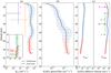 |
Fig. 3 Global mean results. (a) The derived global mean Kzz by adopting LCPS particle distributions. The blue line represents the median value along with the upper and lower quartiles. The derived Kzz profile below 46.5 km is distinguished in red since it is basically constituted of data from the polar regions and better considered as the “polar mean.” The bottom-left subplot displays the Kzz below the clouds, which is based on the given column production of H2SO4 vapor. The red line represents the below-cloud Kzz estimated in polar regions and the green line represents the other regions. The estimations based on Vega balloon observations (fuchsia, Blamont et al. 1986), Pioneer Venus radio scintillation measurements (black, Woo et al. 1982), and model results of McGouldrick & Toon (2007, purple) and Lefèvre et al. (2022, orange) are also presented. (b) The distribution of H2SO4 vapor upward diffusion flux. (c) The derived H2SO4 vertical molecular (left) and eddy (right) diffusion velocities as functions of altitude. The observations of atmospheric convection velocities from Vega balloons (fuchsia, Linkin et al. 1986), as well as model estimations of Imamura et al. (2014, green), Lefèvre et al. (2018, gray), and Gierasch et al. (1997, orange triangles for the Hadley velocity and black stars for the convective velocity) are also presented. |
3 Results
3.1 Global average
The derived global mean Kzz profile is presented in Fig. 3a. The particle distribution used for this estimation was adopted from LCPS observations. According to the results, the cloud Kzz has a peak of 5 × 108 cm2 s−1 near 48 km. Between 50 and 54 km, it remains nearly constant at 2.5 × 108 cm2 s−1 before exhibiting a rapid decrease as the altitude increases above 54 km. This profile is larger than the results obtained from the latest 3D convection-resolving model (Lefèvre et al. 2022) by a factor of three in the middle cloud region, and is roughly an order of magnitude larger than the estimation based on VeRa measurements (Blamont et al. 1986; Sagdeev et al. 1986) at 54 km and the microphysical model (McGouldrick & Toon 2007) above 50 km. The Kzz quickly decreases above 54 km, being consistent with the observed increase in the static stability reported by Akatsuki (Imamura et al. 2017) and the model estimations by Lefèvre et al. (2022). This altitude typically represents the upper boundary of the middle clouds, where the number density of large particles decreases rapidly (Knollenberg & Hunten 1980), thereby weakening the condensation of H2SO4. Notably, a significant enhancement of Kzz is presented within the altitude range of 46.5–49.5 km, corresponding to the altitudes of the lower clouds (Knollenberg & Hunten 1980). The derived Kzz profile below 46.5 km in Fig. 3a is distinguished by another color, for the cloud base in the polar regions (>60 or <−60 degree) could descend to 43 km, while it is averaged at 46.5 km in middle and low latitudes. Since the bottom boundary of our domain is the cloud base, the results in 43–46.5 km are basically made up of data in the polar regions. Thus, it is better considered as a “polar mean.” Detailed results about the latitudinal variations are posted later in this section.
The estimated Kzz profiles below the cloud base (distinguished by polar and other latitudes) are displayed in the subplot of Fig. 3a. The H2SO4 vapor is continuously produced by a chemical process near the cloud top and thermally decomposed in the lower atmospheres (Krasnopolsky 2007, 2012), leading to a net downward flux of total H2SO4. This flux is suggested by a photochemical model (excluding cloud formation) as about 1 × 1012 cm−2 s−1 in our domain (Yung & Demore 1982). In the cloud regions, this net flux is contributed to by both the downward transport of liquid H2SO4 and the upward diffusion of the vapor. A recent microphysical model study (Gao et al. 2014) derived both the downward and upward fluxes on the order of 1 × 1014 cm−2 s−1 in the clouds. They are dramatically larger than the net flux, indicating the strong internal H2SO4 cycle. This difference could even increase by adopting larger cloud Kzz values in their model. In the region shortly below the cloud base, the liquid H2SO4 is not able to contribute to this flux. Then we could expect the total flux to be completely made up of the vapor flux, given that both the chemical production and loss of vapor are weak in this region. To calculate these profiles, we adopted a constant downward H2SO4 vapor flux of 1 × 1012 cm−2 s−1 in a short distance below the cloud base. In this particular region, the H2SO4 vapor abundance is primarily controlled by the vertical transport and its column production, as its thermal decomposition becomes significant below 38 km (Jenkins et al. 1994). The results show that the Kzz is around 1 × 103 cm2 s−1 below the cloud base, increasing slightly with increasing altitude, agreeing with the estimate based on Pioneer Venus radio scintillation measurements at 45 km (Woo et al. 1982). We note that this Kzz profile is displayed for the purpose of indicating that there could be a sharp decrease of Kzz below the cloud base and supporting the comparison of different latitudes later. Since the transition region near the cloud base is not considered in this study, this profile is not connected to the profile in the clouds.
To investigate the vertical motions in the cloud region more comprehensively, we have illustrated the upward diffusion flux of H2SO4 vapor in Fig. 3b, along with its eddy and molecular diffusion velocities shown in Fig. 3c. In 46.5–48.5 km (the lower cloud region), H2SO4 vapor exhibits an upward flux on the order of 1017 cm−2 s−1. Here, we provide a simple estimate to elucidate this outcome. The diameter of mode-3 particles, which are concentrated in this region, is approximately ten times larger than that of mode-1 and mode-2 particles that dominate in the upper clouds. We note that the Stokes velocity of sedimentation is proportional to the square of the particle diameter. Additionally, the mass loading of the lower clouds is roughly 100 times greater than that of the upper clouds (Knollenberg & Hunten 1980). These factors suggest that the sedimentation flux of liquid H2SO4 in the lower clouds is significantly enhanced by four orders of magnitude compared to the upper clouds. Given that the liquid H2SO4 has a sedimentation flux of 1 × 1012 cm−2 s−1 at the transition between the middle and upper clouds (Imamura & Hashimoto 2001; Yung & Demore 1982), an estimated sedimentation flux of liquid H2SO4 in the lower clouds would be approximately 1×1016 cm−2 s−1. Generally, for mass conservation, the downward liquid H2SO4 flux resulting from both sedimentation and diffusion of the particles is equal to the upward vapor diffusion flux. The estimated sedimentation flux is an order of magnitude smaller than our results. This discrepancy can be attributed to the effect of the diffusion of different-sized particles, which it is hard to physically estimate.
The eddy diffusion of H2SO4 vapor yields a velocity on the order of 102−103 cm s−1. It is consistent with the model-estimated Hadley velocity in 52–54 km (Gierasch et al. 1997), but it is two to eight times faster than the convection velocities measured by Vega balloons (Linkin et al. 1986) and convection models (Imamura et al. 2014; Lefèvre et al. 2018). Here, we note that the eddy diffusion in this study characterizes varying processes that drive the atmospheric mixing, incorporating convection, turbulence, and waves. Such a discrepancy might indicate that other processes besides convection also contribute to the eddy mixing of H2SO4 vapor. Eddy diffusion plays a crucial role in the formation of these cloud layers. The H2SO4 vapor generated by evaporation below the cloud base is rapidly transported upward by eddy diffusion, and subsequently condenses back into the droplets within this region (Dai et al. 2022b). Therefore, strong eddy diffusion contributes to a high condensation efficiency in the clouds. This internal cycle is essential for the observed accumulation of mass loading (Knollenberg & Hunten 1980) in the lower and middle clouds (Imamura & Hashimoto 2001; McGouldrick 2017).
The molecular diffusion velocity of H2SO4 vapor ranges from 1 × 10⁻⁶ to 1 × 10⁻⁵ cm s−1. Its magnitude is significantly weaker compared to eddy diffusion in the cloud region, as expected, since our domain is far below the homopause (120–140 km).
3.2 Latitudinal variation
To investigate the latitudinal variation in the Venusian cloud eddy diffusion, we used particle distributions from the latest microphysical model (McGouldrick & Barth 2023), specifically tailored for different latitudes. Although LCPS observations are more reliable than model results, they cannot distinguish latitudinal variations in particle distributions that could influence the condensation rate. Using LCPS data might overlook some critical features. We categorized the latitudes into three bins, covering both hemispheres: 0°–30°, 30°–60°, and 60°–90°. The corresponding Kzz, flux, and velocity profiles generated for each bin are illustrated in Figs. 4a,b,c, respectively, while the altitude-latitude distribution is depicted in Fig. 4d.
The typical cloud-base altitude in polar regions is expected to be 43 km, notably lower than that projected in middle and low latitudes. This is consistent with the measurements obtained by VIRTIS on board Venus Express (Barstow et al. 2012). At the cloud regions in middle and low latitudes, the Kzz is generally comparable, except for a layer situated near 48 km, where the Kzz in middle latitudes exceeds that in low latitudes by a factor of 50%. In 46.5–50 km, the cloud Kzz in polar regions is lower than that in low latitudes, with a typical value of ~8 × 107 cm2 s−1. This seems to contradict some model studies (e.g., Ando et al. 2020b) in which equatorial static stability is higher than that in polar regions. It is reasonable, since Kzz characterizes varying processes that contribute to the atmospheric mixing, including convection. The correlation between Kzz and static stability depends on its relative contribution to the atmospheric motion. For instance, at low latitudes, the global circulation might have some contribution and increase the cloud Kzz in this region. Besides, the derived Kzz in polar regions exhibits a notable enhancement at deeper altitudes, with a peak of 3×108 cm2 s−1 at 43 km, corresponding to the altitude of the lower clouds in the polar regions (Barstow et al. 2012). Although our domain only extends to the cloud base, we can anticipate that the Kzz below this level is several orders lower than the cloud Kzz, as previously mentioned. The bottom of the high-Kzz region significantly shifts from 46.5 km at the equator to 43 km in polar regions (as depicted in Fig. 4d). This altitudinal variation is consistent with the static stability distributions obtained from VeRa measurements (Ando et al. 2015, Ando et al. 2020a), where the low static stability region extends down to 42 km at high latitudes.
The upward diffusion fluxes of H2SO4 vapor above 46.5 km exhibit a significant decrease as the latitude increases. As we have mentioned above, this might be related to the effect of global circulation. The flux basically decreases with increasing altitude at all latitudes. It peaks at 47.5 km in low latitudes, with a value of 1.5 × 1017 cm−2 s−1. Below 46.5 km, the fluxes in middle and low latitudes could be expected to rapidly decrease as Kzz decreases, while the flux in polar regions reaches a peak at 44 km, with a value of 1 × 1017 cm−2 s−1. The agreement with observed low polar static stability in 43–46.4 km (Ando et al. 2015, Ando et al. 2020a) indicates that convection might regulate the H2SO4 vapor mixing in this region. The latitudinal variation in the eddy diffusion velocity is not significant. It increases as the altitude increases on the order of several m s−1 and reaches a peak at 53 km on the order of 10 m s−1. It inverses above 53 km as the decreasing particle size reduces the condensation rate.
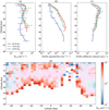 |
Fig. 4 Latitudinal variation. (a) Kzz, (b) H2SO4 vapor upward diffusion flux, and (c) H2SO4 vapor eddy diffusion velocity profiles in different latitude bins were derived by adopting particle distributions from the microphysical model results (McGouldrick & Barth 2023). The red, green, and blue lines represent the latitudinal bins of 0°–30°, 30°–60°, and 60°–90°, respectively. Panel d presents the altitude-latitude distribution of derived Kzz. We note that the missing middle-latitude results near 47 km are caused by a lack of data. |
4 Discussion
A 1D photochemistry-diffusion model (Rimmer et al. 2021) has been used to evaluate the measured Kzz in the Venusian clouds. Here we only summarize the key points of the model. More details can be found in Rimmer et al. (2021). This model includes over 3000 reactions involving 480 species. It solves the continuity equations containing eddy mixing and chemistry at each altitude. Furthermore, it performs the cloud formation and tracks the SO2 dissolution based on Henry’s Law and the presence of hydroxide salts. By incorporating our derived global mean cloud Kzz (46.5–55 km) into their nominal profile, we made comparisons of several species. The results are shown in Fig. 5. We note that the discontinuous patchwork of Kzz profiles in Fig. 5a has a 4-order of magnitude enhancement in a 10-km region that does not take the transition regions near the intersections of two Kzz profiles into account. A similar pattern of Kzz distribution is indicated by the results of a 3D convection-resolving model (Lefèvre et al. 2022).
By adopting a high-Kzz profile in the Venusian clouds, the simulated vapor profiles of SO2, H2O, SO, and CO are in good agreement with observations, with the exception of a slightly lower CO mixing ratio above 65 km. These indicate that the presence of a high-Kzz layer in the clouds may not significantly affect the overall profiles of these species. Comparing these results to the nominal case presented in Rimmer et al. (2021, hereafter R21), we gain an insight into the role played by cloud Kzz. While previous studies such as Bierson & Zhang (2020) emphasize the significant influence of cloud Kzz on the vertical transport of SO2, our × 104 enhancement of cloud Kzz in R21 does not induce a suppression of the SO2 depletion at 57 km (Fig. 5b). This can be attributed to the fact that the depletion is primarily regulated by the dissolution of SO2 into the droplets, a process accounted for in R21 but not in the study by Bierson & Zhang (2020), which does not include cloud formation. A similar behavior has occurred to H2O depletion (Fig. 5c), indicating its connection to cloud formation.
Interestingly, empirical estimates of cloud Kzz in 1D chemical models that exclude cloud formation (e.g., Bierson & Zhang 2020) usually yield lower values compared to those obtained from cloud models (e.g., Gao et al. 2014; McGouldrick 2017). The vertical distributions of certain species such as SO2 in the former studies exhibit a higher sensitivity to the cloud Kzz. It appears that the Venusian clouds act as a large reservoir for related vapors, buffering their abundances in response to variations in vertical transport. In order to satisfy mass conservation, the cloud mass loading must vary with the cloud Kzz. This hypothesis is supported by our simulation, in which the mixing ratio of liquid H2SO4 significantly increases with the enhancement of cloud Kzz (Fig. 5d). The derived several-ppm liquid H2SO4 in the clouds agrees with Dai et al. (2022b). To further validate this hypothesis, it is crucial to conduct additional investigations into the material exchange between the clouds and the atmosphere.
In contrast to SO2 and H2O, the distributions of both SO and CO in the cloud region appear to be more uniform in the case of enhanced cloud Kzz compared to R21 (Figs. 5e–f). It indicates that the cloud Kzz can still have an impact on these species independently of cloud formation in this region.
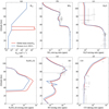 |
Fig. 5 Evaluation of measured Kzz by adopting a 1D photochemistry-diffusion model (Rimmer et al. 2021). (a) The Kzz profiles in this study (red) and in Rimmer et al. (2021, blue). (b–f) Simulated vapor mixing ratio profiles of SO2, H2O, H2SO4 (liquid), SO, and CO, respectively (credit: Sean Jordan). The observations are shown as gray lines and scatters. |
5 Conclusions
We estimated the Kzz between the cloud base and 55 km using H2SO4 vapor mixing ratios derived from the observations of VeRa on board Venus Express. Our approach relies on the premise that H2SO4 vapor is primarily regulated by diffusion and condensation processes in this region. The obtained global mean cloud Kzz exhibits distinct characteristics: it peaks at 5 × 108 cm2 s−1 near 48 km, remains relatively constant at 2.5 × 108 cm2 s−1 between 50 and 54 km, and rapidly decreases above that altitude. The measured Kzz is larger than model results (Lefèvre et al. 2022) by a factor of three and larger than evaluations of Vega (Blamont et al. 1986) and a microphysical model (McGouldrick & Toon 2007) by an order of magnitude. Besides, the vertical eddy motion exhibits a mean velocity on the order of 102−103 cm s−1, which is two to eight times larger than the measurements of Vega balloons (Linkin et al. 1986) and convection models (Imamura et al. 2014; Lefèvre et al. 2018), suggesting that large-scale motions contribute significantly to the effective vertical eddy motions.
Our results suggest that cloud Kzz exhibits significant latitudinal variation. Although equatorial Kzz is three times as large as polar Kzz at 48 km, the high-Kzz layer in the polar regions can extend down to 43 km, with a peak Kzz of 1 × 108 cm2 s−1 at 43.5 km. This altitudinal variation is consistent with the static stability distribution obtained from VeRa measurements (Ando et al. 2015, 2020a). However, our polar Kzz in the region above 46.5 km is lower than the equatorial Kzz, which seems to contradict the static stability distributions in some model studies (e.g., Ando et al. 2020b). This could be explained by other processes besides convection contributing to the H2SO4 vapor mixing in this region, such as global circulation. The upward diffusion flux of H2SO4 vapor above 46.5 km significantly decreases as the latitude increases. The flux in middle and low latitudes peaks at 48 km with a value of 1.5 × 1017 cm−2 s−1 while polar flux reaches a peak at 44 km with a value of 1.5 × 1017 cm−2 s−1. The latitudinal variation of eddy diffusion velocity is not significant.
To evaluate our results, we integrated the derived global mean Kzz in 46.5–55 km into the latest 1D photochemistry-diffusion model developed by Rimmer et al. (2021). The simulated distributions of SO2, H2O, SO, and CO are in good agreement with observations, except for a slight underestimation of the CO mixing ratio above 65 km. Our simulations indicate that the enhancement of cloud Kzz does not suppress the depletions of SO2 and H2O, but does significantly mix SO and CO in the cloud regions. Additionally, the enhancement of cloud Kzz largely increases the cloud mass loading. This indicates that the clouds could act as reservoirs for related vapors, buffering their abundances by adjusting the cloud mass loading in response to variations in vertical transport. Further investigations on the material exchange between the Venusian clouds and atmosphere are essential to verify this hypothesis.
Acknowledgments
We thank Janusz Oschlisniok (University of Cologne) for providing H2SO4 vapor data from VeRa observations, Kevin McGouldrick (University of Colorado Boulder) for providing particle distribution data from their public model results, Sean Jordan (University of Cambridge) for providing the output of their photochemistry-diffusion model. We thank the anonymous reviewer for his thoughtful suggestions that greatly improve the quality of our manuscript. This work is supported by the National Natural Science Foundation of China (Grant 42305135, 42275060). Longkang Dai is supported by Natural Science Foundation of Hunan Province (Grant 2023JJ40664). The data in this study are publically available at https://doi.org/10.6084/m9.figshare.24160752.V1.
Appendix A Uncertainty due to the retrieved H2SO4 profiles
The uncertainties produced by zonal data statistics in our cloud Kzz estimation have been exhibited in the figures. However, additional errors might be carried by H2SO4 vapor data. According to Oschlisniok et al. (2021), the absorption of SO2 has been removed from the raw data by the estimated SO2 abundance, and the SO2 absorption is small compared to the H2SO4 absorption. Further testing from the authors shows that a 60-ppm increase or decrease in SO2 could lead to about a 6% increase or decrease in the H2SO4 vapor in the lower clouds. Here we adopted a column variation of 6% H2SO4 vapor in the same cases in Figure 2. The derived H2SO4 vapor diffusion flux, the condensation or evaporation rate, and Kzz profiles are presented in Figure A.1. It shows that the effect on the H2SO4 vapor diffusion flux increases as the altitude decreases. 6% H2SO4 vapor column uncertainty results in a lower-cloud flux deviation of 1×1017 cm−2 s−1 in low latitudes and 4×1016 cm−2 s−1 in high latitudes. The effect on Kzz also increases with both decreasing altitude and latitude. Its uncertainty due to the retrieved H2SO4 profiles reaches 22.88% at 47.8 km in low latitudes and 8.92% at 44 km in high latitudes.
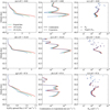 |
Fig. A.1 Uncertainty tests on corresponding cases in Figure 2. The left, middle, and right columns show H2SO4 vapor diffusion flux, the condensation or evaporation rate, and Kzz profiles, respectively. The green lines represent the original data. The red lines represent a 6% increase in the H2SO4 vapor column. The blue lines represent a 6% decrease in the H2SO4 vapor column. |
References
- Ando, H., Imamura, T., Tsuda, T., et al. 2015, J. Atmos. Sci., 72, 2318 [NASA ADS] [CrossRef] [Google Scholar]
- Ando, H., Imamura, T., Tellmann, S., et al. 2020a, Sci. Rep., 10, 3448 [Google Scholar]
- Ando, H., Takagi, M., Sugimoto, N., Sagawa, H., & Matsuda, Y. 2020b, J. Geophys. Res. (Planets), 125, e06208 [Google Scholar]
- Ando, H., Takaya, K., Takagi, M., et al. 2022, J. Geophys. Res. (Planets), 127, e06957 [Google Scholar]
- Arney, G., Meadows, V., Crisp, D., et al. 2014, J. Geophys. Res. (Planets), 119, 1860 [NASA ADS] [CrossRef] [Google Scholar]
- Barstow, J. K., Tsang, C. C. C., Wilson, C. F., et al. 2012, Icarus, 217, 542 [NASA ADS] [CrossRef] [Google Scholar]
- Bierson, C. J., & Zhang, X. 2020, J. Geophys. Res. (Planets), 125, e06159 [NASA ADS] [Google Scholar]
- Blamont, J. E., Young, R. E., Seiff, A., et al. 1986, Science, 231, 1422 [NASA ADS] [CrossRef] [Google Scholar]
- Dai, L., Zhang, X., & Cui, J. 2022a, MNRAS, 515, 817 [NASA ADS] [CrossRef] [Google Scholar]
- Dai, L., Zhang, X., Shao, W. D., Bierson, C. J., & Cui, J. 2022b, J. Geophys. Res. (Planets), 127, e07060 [Google Scholar]
- Esposito, L. W., Knollenberg, R. G., Marov, M. I., Toon, O. B., & Turco, R. P. 1983, in Venus (Tucson: University of Arizona Press), 484 [Google Scholar]
- Gao, P., Zhang, X., Crisp, D., Bardeen, C. G., & Yung, Y. L. 2014, Icarus, 231, 83 [NASA ADS] [CrossRef] [Google Scholar]
- Gierasch, P. J., Goody, R. M., Young, R. E., et al. 1997, in Venus II: Geology, Geophysics, Atmosphere, and Solar Wind Environment, eds. S. W. Bougher, D. M. Hunten, & R. J. Phillips (Tucson: University of Arizona Press), 459 [Google Scholar]
- Hamill, P., Toon, O. B., & Kiang, C. S. 1977, J. Atmos. Sci., 34, 1104 [NASA ADS] [CrossRef] [Google Scholar]
- Hanson, D. R., & Eisele, F. 2000, J. Phys. Chem. A, 104, 1715 [NASA ADS] [CrossRef] [Google Scholar]
- Hinson, D. P., & Jenkins, J. M. 1995, Icarus, 114, 310 [NASA ADS] [CrossRef] [Google Scholar]
- Imamura, T., & Hashimoto, G. L. 2001, J. Atmos. Sci., 58, 3597 [NASA ADS] [CrossRef] [Google Scholar]
- Imamura, T., Higuchi, T., Maejima, Y., et al. 2014, Icarus, 228, 181 [Google Scholar]
- Imamura, T., Ando, H., Tellmann, S., et al. 2017, Earth Planets Space, 69, 137 [NASA ADS] [CrossRef] [Google Scholar]
- Imamura, T., Mitchell, J., Lebonnois, S., et al. 2020, Space Sci. Rev., 216, 87 [NASA ADS] [CrossRef] [Google Scholar]
- Jenkins, J. M., Steffes, P. G., Hinson, D. P., Twicken, J. D., & Tyler, G. L. 1994, Icarus, 110, 79 [NASA ADS] [CrossRef] [Google Scholar]
- Kerzhanovich, V. V., & Marov, M. I. 1983, in Venus (Tucson: University of Arizona Press), 766 [Google Scholar]
- Knollenberg, R. G., & Hunten, D. M. 1980, J. Geophys. Res., 85, 8039 [CrossRef] [Google Scholar]
- Krasnopolsky, V. A. 2007, Icarus, 191, 25 [NASA ADS] [CrossRef] [Google Scholar]
- Krasnopolsky, V. A. 2012, Icarus, 218, 230 [NASA ADS] [CrossRef] [Google Scholar]
- Krasnopolsky, V. A. 2015, Icarus, 252, 327 [NASA ADS] [CrossRef] [Google Scholar]
- Kulmala, M., & Laaksonen, A. 1990, J. Chem. Phys., 93, 696 [NASA ADS] [CrossRef] [Google Scholar]
- Lefèvre, M., Lebonnois, S., & Spiga, A. 2018, J. Geophys. Res. (Planets), 123, 2773 [CrossRef] [Google Scholar]
- Lefèvre, M., Marcq, E., & Lefèvre, F. 2022, Icarus, 386, 115148 [CrossRef] [Google Scholar]
- Limaye, S. S., Grassi, D., Mahieux, A., et al. 2018, Space Sci. Rev., 214, 102 [NASA ADS] [CrossRef] [Google Scholar]
- Linkin, V. M., Kerzhanovich, V. V., Lipatov, A. N., et al. 1986, Science, 231, 1417 [NASA ADS] [CrossRef] [Google Scholar]
- Mahieux, A., Yelle, R. V., Yoshida, N., et al. 2021, Icarus, 361, 114388 [NASA ADS] [CrossRef] [Google Scholar]
- McGouldrick, K. 2017, Earth Planets Space, 69, 161 [NASA ADS] [CrossRef] [Google Scholar]
- McGouldrick, K., & Barth, E. L. 2023, Planet. Sci. J., 4, 50 [NASA ADS] [CrossRef] [Google Scholar]
- McGouldrick, K., & Toon, O. B. 2007, Icarus, 191, 1 [NASA ADS] [CrossRef] [Google Scholar]
- Mehio, N., Dai, S., & Jiang, D.-e. 2014, J. Phys. Chem. A, 118, 1150 [NASA ADS] [CrossRef] [Google Scholar]
- Myhre, C. E., Nielsen, C. J., & Saastad, O. W. 1998, J. Chem. Eng. Data, 43, 617 [CrossRef] [Google Scholar]
- Oschlisniok, J., Häusler, B., Pätzold, M., et al. 2021, Icarus, 362, 114405 [NASA ADS] [CrossRef] [Google Scholar]
- Palmer, K. F., & Williams, D. 1975, Appl. Opt., 14, 208 [NASA ADS] [CrossRef] [Google Scholar]
- Rimmer, P. B., Jordan, S., Constantinou, T., et al. 2021, Planet. Sci. J., 2, 133 [NASA ADS] [CrossRef] [Google Scholar]
- Sagdeev, R. Z., Linkin, V. M., Kerzhanovich, V. V., et al. 1986, Science, 231, 1411 [NASA ADS] [CrossRef] [Google Scholar]
- Savitzky, A., & Golay, M. J. E. 1964, Analyt. Chem., 36, 1627 [NASA ADS] [CrossRef] [Google Scholar]
- Schafer, R. 2011, IEEE Signal Process. Mag., 28, 111 [NASA ADS] [CrossRef] [Google Scholar]
- Seinfeld, J. H., & Pandis, S. N. 2016, Atmospheric Chemistry and Physics: From Air Pollution to Climate Change (Hoboken, NJ, USA: John Wiley & Sons) [Google Scholar]
- Shao, W. D., Zhang, X., Bierson, C. J., & Encrenaz, T. 2020, J. Geophys. Res. (Planets), 125, e06195 [Google Scholar]
- Steffes, P. G., & Eshleman, V. R. 1982, Icarus, 51, 322 [NASA ADS] [CrossRef] [Google Scholar]
- Stolzenbach, A., Lefèvre, F., Lebonnois, S., & Määttänen, A. 2023, Icarus, 395, 115447 [NASA ADS] [CrossRef] [Google Scholar]
- Swenson, G. R., Salinas, C. C. J. H., Vargas, F., et al. 2019, J. Geophys. Res. (Atmos.), 124, 13519 [CrossRef] [Google Scholar]
- Titov, D. V., Ignatiev, N. I., McGouldrick, K., Wilquet, V., & Wilson, C. F. 2018, Space Sci. Rev., 214, 126 [NASA ADS] [CrossRef] [Google Scholar]
- Turbet, M., Bolmont, E., Chaverot, G., et al. 2021, Nature, 598, 276 [CrossRef] [Google Scholar]
- von Zahn, U., Fricke, K. H., Hunten, D. M., et al. 1980, J. Geophys. Res., 85, 7829 [CrossRef] [Google Scholar]
- Woo, R., & Ishimaru, A. 1981, Nature, 289, 383 [NASA ADS] [CrossRef] [Google Scholar]
- Woo, R., Armstrong, J. W., & Kliore, A. J. 1982, Icarus, 52, 335 [NASA ADS] [CrossRef] [Google Scholar]
- Yoshida, N., Nakagawa, H., Aoki, S., et al. 2022, Geophys. Res. Lett., 49, e98485 [NASA ADS] [CrossRef] [Google Scholar]
- Yung, Y. L., & Demore, W. B. 1982, Icarus, 51, 199 [NASA ADS] [CrossRef] [Google Scholar]
- Zeleznik, F. J. 1991, J. Phys. Chem. Ref. Data, 20, 1157 [NASA ADS] [CrossRef] [Google Scholar]
- Zhang, X., & Showman, A. P. 2018, ApJ, 866, 1 [NASA ADS] [CrossRef] [Google Scholar]
- Zhang, X., Liang, M. C., Mills, F. P., Belyaev, D. A., & Yung, Y. L. 2012a, Icarus, 217, 714 [NASA ADS] [CrossRef] [Google Scholar]
- Zhang, X., Pandis, S. N., & Seinfeld, J. H. 2012b, Aerosol Sci. Technol., 46, 874 [NASA ADS] [CrossRef] [Google Scholar]
All Tables
All Figures
|
Fig. 1 VeRa observations (Oschlisniok et al. 2021). The panels show (a) the H2SO4 vapor volume mixing ratio, (b) temperature, and (c) pressure, respectively. We note that these observations are divided into 36 latitudinal bins with a resolution of 5 degrees. The lack of measurements is caused by the orbit geometry of Venus Express. |
| In the text | |
|
Fig. 2 Example cases illustrating the method of Kzz estimation. The three rows refer to (a–c) −0.02°, (d–f) −52.65°, and (g–i) 87.8° latitude, respectively. The left column shows the original H2SO4 vapor mixing ratio (VMR, solid black line), smoothed H2SO4 vapor mixing ratio (solid red line), and saturation vapor mixing ratio (SVMR, dashed black line) profiles. The middle column shows the net condensation (blue line) and evaporation (red line) rate profiles. The right column shows the derived Kzz distributions. The red triangles represent negative values, caused by the statistical fluctuation and horizontal convergence or divergence of H2SO4 vapor. |
| In the text | |
|
Fig. 3 Global mean results. (a) The derived global mean Kzz by adopting LCPS particle distributions. The blue line represents the median value along with the upper and lower quartiles. The derived Kzz profile below 46.5 km is distinguished in red since it is basically constituted of data from the polar regions and better considered as the “polar mean.” The bottom-left subplot displays the Kzz below the clouds, which is based on the given column production of H2SO4 vapor. The red line represents the below-cloud Kzz estimated in polar regions and the green line represents the other regions. The estimations based on Vega balloon observations (fuchsia, Blamont et al. 1986), Pioneer Venus radio scintillation measurements (black, Woo et al. 1982), and model results of McGouldrick & Toon (2007, purple) and Lefèvre et al. (2022, orange) are also presented. (b) The distribution of H2SO4 vapor upward diffusion flux. (c) The derived H2SO4 vertical molecular (left) and eddy (right) diffusion velocities as functions of altitude. The observations of atmospheric convection velocities from Vega balloons (fuchsia, Linkin et al. 1986), as well as model estimations of Imamura et al. (2014, green), Lefèvre et al. (2018, gray), and Gierasch et al. (1997, orange triangles for the Hadley velocity and black stars for the convective velocity) are also presented. |
| In the text | |
|
Fig. 4 Latitudinal variation. (a) Kzz, (b) H2SO4 vapor upward diffusion flux, and (c) H2SO4 vapor eddy diffusion velocity profiles in different latitude bins were derived by adopting particle distributions from the microphysical model results (McGouldrick & Barth 2023). The red, green, and blue lines represent the latitudinal bins of 0°–30°, 30°–60°, and 60°–90°, respectively. Panel d presents the altitude-latitude distribution of derived Kzz. We note that the missing middle-latitude results near 47 km are caused by a lack of data. |
| In the text | |
|
Fig. 5 Evaluation of measured Kzz by adopting a 1D photochemistry-diffusion model (Rimmer et al. 2021). (a) The Kzz profiles in this study (red) and in Rimmer et al. (2021, blue). (b–f) Simulated vapor mixing ratio profiles of SO2, H2O, H2SO4 (liquid), SO, and CO, respectively (credit: Sean Jordan). The observations are shown as gray lines and scatters. |
| In the text | |
|
Fig. A.1 Uncertainty tests on corresponding cases in Figure 2. The left, middle, and right columns show H2SO4 vapor diffusion flux, the condensation or evaporation rate, and Kzz profiles, respectively. The green lines represent the original data. The red lines represent a 6% increase in the H2SO4 vapor column. The blue lines represent a 6% decrease in the H2SO4 vapor column. |
| In the text | |
Current usage metrics show cumulative count of Article Views (full-text article views including HTML views, PDF and ePub downloads, according to the available data) and Abstracts Views on Vision4Press platform.
Data correspond to usage on the plateform after 2015. The current usage metrics is available 48-96 hours after online publication and is updated daily on week days.
Initial download of the metrics may take a while.