| Issue |
A&A
Volume 698, June 2025
|
|
|---|---|---|
| Article Number | A234 | |
| Number of page(s) | 13 | |
| Section | Extragalactic astronomy | |
| DOI | https://doi.org/10.1051/0004-6361/202453267 | |
| Published online | 17 June 2025 | |
Evolution of the UV slope of galaxies at cosmic morning (z > 4): The properties of extremely blue galaxies
1
INAF – Osservatorio Astronomico di Roma, via Frascati 33, 00078 Monte Porzio Catone, Italy
2
Università di Roma ‘La Sapienza’, piazzale Aldo Moro 5, 00185 Roma, Italy
3
Institute of Science and Technology Austria (ISTA), Am Campus 1, A-3400 Klosterneuburg, Austria
4
Department of Astronomy, University of Geneva, Chemin Pegasi 51, 1290 Versoix, Switzerland
5
Instituto de Astrofísica de Andalucía (CSIC), Apartado 3004, 18080 Granada, Spain
6
ARAID Foundation, Centro de Estudios de Física del Cosmos de Aragón (CEFCA), Unidad Asociada al CSIC, Plaza San Juan 1, E-44001 Teruel, Spain
7
NSF’s National Optical-Infrared Astronomy Research Laboratory, 950 N. Cherry Ave., Tucson, AZ 85719, USA
8
Space Telescope Science Institute, 3700 San Martin Drive, Baltimore, MD 21218, USA
9
Institute of Physics, Laboratory of Galaxy Evolution, Ecole Polytechnique Fédérale de Lausanne (EPFL), Observatoire de Sauverny, 1290 Versoix, Switzerland
10
Department of Astronomy, The University of Texas at Austin, 2515 Speedway, Austin, TX 78712, USA
11
Center for Astrophysics | Harvard & Smithsonian, 60 Garden St., Cambridge, MA 02138, USA
12
Black Hole Initiative at Harvard University, 20 Garden St., Cambridge, MA 02138, USA
13
Astronomy Centre, University of Sussex, Falmer, Brighton BN1 9QH, UK
14
Institute of Space Sciences and Astronomy, University of Malta, Msida, MSD 2080, Malta
15
Astrophysics Science Division, NASA Goddard Space Flight Center, 8800 Greenbelt Rd, Greenbelt, MD 20771, USA
16
Laboratory for Multiwavelength Astrophysics, School of Physics and Astronomy, Rochester Institute of Technology, 84 Lomb Memorial Drive, Rochester, NY 14623, USA
17
George P. and Cynthia Woods Mitchell Institute for Fundamental Physics and Astronomy, Texas A&M University, College Station TX 77843-4242, USA
18
Department of Physics and Astronomy, Texas A&M University, College Station, TX 77843-4242, USA
19
ESA/AURA, Space Telescope Science Institute, 3800 San Martin Drive, Baltimore, MD 21218, USA
⋆ Corresponding author.
Received:
2
December
2024
Accepted:
21
April
2025
Abstract
We present an analysis of the UV continuum slope, β, using a sample of 726 galaxies with z > 4, selected from a mixture of JWST ERS, GTO, and GO observational programs. We considered only spectroscopic data obtained with the low-resolution (R ∼ 30 − 300) PRISM/CLEAR NIRSpec configuration. Studying the correlation between β and MUV, we find an overall decreasing trend, described by β = ( − 0.055 ± 0.017)MUV + ( − 2.98 ± 0.34). This is consistent with previous studies, where brighter galaxies show redder β values. However, when analyzing the trend in separate redshift bins, we find that at high redshift the relation becomes much flatter and is consistent with a flat slope within 1σ. Furthermore, we find that β tends to decrease with redshift, following β = ( − 0.075 ± 0.010)z + ( − 1.496 ± 0.056). This is consistent with most recent results showing a steepening of the spectra at higher z. We selected a sample of galaxies with extremely blue slopes (i.e., β < −2.6). Such slopes are steeper than predicted by stellar evolution models – even for dust-free, young, metal-poor populations – when the contribution of nebular emission is included. We selected 44 extremely blue galaxies (XBGs) and investigated the possible physical origin of their steep slopes by comparing them to a subsample of redder galaxies (matched in Δz = ±0.5 and ΔMUV = ±0.2). We find that XBGs have younger stellar populations, stronger ionization fields, lower dust attenuation, and lower but not pristine metallicity (∼10% Z⊙) compared to red galaxies. However, these properties alone cannot explain the extreme β values. Using indirect inference of Lyman continuum escape with the most recent models, we estimated the escape fraction fesc > 10% in at least 25% of the XBGs, whereas all the red sources exhibit much lower fesc values. A reduced nebular continuum contribution – resulting from either a high escape fraction or a bursty star formation history – is likely the origin of the extremely blue slopes.
Key words: galaxies: evolution / galaxies: high-redshift / galaxies: ISM / galaxies: star formation / galaxies: statistics
NASA Postdoctoral Fellow.
© The Authors 2025
 Open Access article, published by EDP Sciences, under the terms of the Creative Commons Attribution License (https://creativecommons.org/licenses/by/4.0), which permits unrestricted use, distribution, and reproduction in any medium, provided the original work is properly cited.
This article is published in open access under the Subscribe to Open model. This email address is being protected from spambots. You need JavaScript enabled to view it. to support open access publication.
1. Introduction
Thanks to its unprecedented sensitivity and resolution, recent JWST observations have probed the most distant galaxies ever detected, offering a direct glimpse into the first stages of galaxy formation and evolution (e.g., Treu et al. 2022; Finkelstein et al. 2023; Adamo et al. 2024). These observations have also been fundamental for studying the process of cosmic reionization between approximately 300 million and 1 billion years after the Big Bang (corresponding to redshifts 14 and 6), during which UV light emitted from the first stars and galaxies reionized the surrounding neutral hydrogen in the intergalactic medium (IGM) (Jones et al. 2024; Napolitano et al. 2024).
A critical observational diagnostic to understand early galaxy evolution and the reionization mechanism is the slope of the UV continuum β. The UV slope characterizes the spectral energy distribution (SED) of a galaxy in the UV range, which is dominated by the emission of massive O/B-type main sequence stars. Defined by the relation fλ ∝ λβ, (Calzetti et al. 1994) where fλ is the flux density at wavelength λ, β provides essential insights into the physical properties of galaxies, including dust content and stellar population properties. β is primarily sensitive to the presence of dust, which can redden the SED and result in a less negative or even positive UV slope (Meurer et al. 1999; Calzetti et al. 2000; Wilkins et al. 2016). It is also directly influenced by the age and metallicity of the stellar populations within a galaxy (see Bouwens et al. 2012; Castellano et al. 2012; Tacchella et al. 2022): younger and more metal-poor galaxies tend to have bluer UV slopes, reflecting the predominance of hot, massive stars. Even though massive Pop III stars can have a significantly blue intrinsic UV spectrum (β < −2.6), their strong nebular continuum emission produces spectral shapes that are redder than those of non-Pop III stellar populations (Raiter et al. 2010; Zackrisson et al. 2011; Trussler et al. 2023). Furthermore, β is also a crucial quantity for studying reionization, as it is related to the fraction of Lyman continuum photons escaping from a galaxy fesc (Mascia et al. 2023; Chisholm et al. 2022), whose direct estimation becomes prohibitive at z > 4 due to the increasingly high opacity of the IGM to the ionizing radiation.
The extensive imaging campaigns conducted by recent surveys with JWST NIRCam (Rieke et al. 2005, 2023) have made it possible to assemble a large statistical sample of photometrically selected galaxies at high redshifts (≥4) and to directly measure their UV slope from photometry. Recent studies have thus investigated the evolution of the UV slope across cosmic time until the epoch of reionization (EoR) (e.g., Topping et al. 2022; Tacchella et al. 2022; Roberts-Borsani et al. 2022; Cullen et al. 2023; Austin et al. 2024). Combining these results with pre-JWST studies (e.g., Finkelstein et al. 2012; Hathi et al. 2013, 2016; Kurczynski et al. 2014; Bouwens et al. 2014; Pilo et al. 2019; Morales et al. 2024), they find that, overall, β decreases on average from cosmic noon (z ≃ 2) to dawn (z ≃ 10) for galaxies with similar stellar masses. In addition, several studies have found that the average UV slope of faint star-forming galaxies (−20 < MUV < −17) at z ≃ 9.5 approaches values of –2.5, which is close to the theoretical lower limit of ≃ − 2.6 produced by pure stellar and nebular continuum emission (Topping et al. 2022; Cullen et al. 2024; Morales et al. 2024). Some studies have reported galaxies with extremely low β values dropping below –3 (e.g., Topping et al. 2022; Atek et al. 2023; Austin et al. 2023; Yanagisawa et al. 2024), although these results may be affected by photometric uncertainties and the limited number of photometric bands used for the β estimation. Such extremely blue slopes can only be explained if nebular emission is suppressed, for example, by the leakage of ionizing radiation (Messa et al. 2025).
Meanwhile, spectroscopic observations with JWST NIRSpec (Jakobsen et al. 2022) have confirmed an increasing number of galaxies in the EoR. These observations have paved the way for a statistical investigation of their physical properties from emission lines, including star formation rates (Calabrò et al. 2024), ionization properties (Reddy et al. 2023; Sanders et al. 2023), and interstellar medium (ISM) metallicities (Nakajima et al. 2023; Curti et al. 2023; Sanders et al. 2024). The NIRSpec spectra have also allowed us for the first time to derive β estimates that are independent of those obtained from photometry alone.
Measuring the UV slopes from the spectra has several advantages. First, we can precisely define the wavelength range for the fit, for example by adopting the original range between the 1250 and 2750 Å rest-frame as defined by Calzetti et al. (1994), in order to exclude the Lyman break on the bluer side and the Balmer break on the redder side. Second, we can identify and mask the bright UV rest-frame emission lines, which might otherwise cause systematic deviations from the true UV slope of the stellar continuum by as much as 0.5–0.6, as shown by Austin et al. (2024). Finally, we can check the spectra for the presence of Lyman-α damping wing absorptions redward of Lyα, which can yield a redder UV slope if the bluest photometric band includes a substantial region close to the Lyα line.
In this work, we assembled a large spectroscopic sample of galaxies at z > 4 to study the evolution of the spectroscopic β during and shortly after the end of the reionization epoch and to compare these results with previous studies based solely on photometry. To this aim, we put together JWST NIRSpec observations from multiple surveys, including the Cosmic Evolution Early Release Science Survey (CEERS, Finkelstein et al. 2023), the JWST Advanced Deep Extragalactic Survey (JADES, Eisenstein et al. 2023), and all other public surveys whose reduced spectra are available through the DAWN JWST Archive (DJA, Heintz et al. 2025). We consider only the spectra taken with the PRISM configuration, which, among all spectroscopic setups, provides the highest S/N on the continuum and is therefore the best suited for the goals of this work.
The paper is structured as follows: In Sect. 2, we describe the observations and methodology, including the sample selection and the measurement of the UV slope β from the PRISM spectra. In Sect. 3, we compare the UV slopes to the UV rest-frame magnitudes of all the galaxies in the sample and study the evolution of β with redshift. We also check for evidence of Lyman-α damping wing absorption in the spectra, which would indicate increasing IGM opacity to Lyα at higher redshifts. In Sect. 4, we identify a subset of extremely blue galaxies (XBGs) with β < −2.6 and investigate the physical origin of their extreme UV slopes by comparing them to a redshift and MUV-matched sample of redder galaxies. Lastly in Sect. 5, we summarize our findings. Throughout the paper, we adopt a Chabrier (2003) initial mass function (IMF), with a solar metallicity of 12 + log(O/H) = 8.69 (Asplund et al. 2009), and assume a standard cosmology with  , Ωm = 0.3, and ΩΛ = 0.7.
2. Methodology
In this study, we considered JWST NIRSpec observations from a series of programs and selected galaxies with a redshift greater than 4 in order to cover the entire rest-frame UV range required for the analysis of the UV slope. This also allowed us to trace the evolution of the β as we approached the reionization epoch. We considered all observations carried out with the PRISM/CLEAR NIRSpec configuration, which offers a wider wavelength coverage (from 0.6 to 5.3 μm) compared to the medium- and high-resolution NIRSpec gratings, as well as significantly higher sensitivity to the continuum. This maximizes the number of sources for which it is possible to measure the UV spectral slope. In the following subsections, we describe the spectroscopic observations used for the analysis, the measurement of the UV slopes, and the final sample selection.
2.1. Spectroscopic observations
We first collected the NIRSpec-PRISM spectra from CEERS (ERS 1345, PI: S. Finkelstein) in the Extended Groth Strip (EGS) field of CANDELS (Grogin et al. 2011; Koekemoer et al. 2011). In the same field, we considered sources from the DDT program 2750 (PI: P. Arrabal Haro). We then added sources from JADES (PI: D. J. Eisenstein) in the Great Observatories Origins Deep Survey (GOODS, Giavalisco et al. 2004) South field and in the GOODS North field. The fully calibrated spectra are publicly available through their third data release (D’Eugenio et al. 2025)1. Lastly, we included galaxies in the GOODS (North and South), COSMOS, EGS, and UDS fields from DJA2 (Heintz et al. 2025), an online repository containing reduced images, photometric catalogs, and spectroscopic data from all public JWST data products. This repository also includes galaxies observed by the BoRG-JWST survey (P.I. Roberts-Borsani et al. 2025). The DJA spectroscopic archive (DJA-Spec) currently comprises observations from several large Early Release Science (ERS), General Observer (GO), and Guaranteed Time (GTO) Cycle 1 & 2 programs. All data processing was performed with the publicly available Grizli (Brammer 2023) and MSAExp (Brammer 2023) software modules. We considered version 2 of the DJA NIRSpec MSA Extractions. For all galaxies, slit loss corrections were applied by default by the JWST pipeline during the reduction process. We did not apply any further photometric corrections to the galaxy spectra. In fact, previous studies show that residual correction factors are significantly modest and do not significantly dependent on wavelength in the range 0.6–3 μm used for the derivation of the UV slopes (Llerena et al. 2024; Calabrò et al. 2024; Roberts-Borsani et al. 2024).
In our analysis, we excluded galaxies located in fields affected by the gravitational lensing of foreground clusters to avoid additional uncertainties arising from magnification. In particular, this effect can substantially bias the absolute magnitude, MUV, used extensively throughout our work – from the β versus Muv relation itself to the definition of key parameters for studying XBGs (e.g., the escape fraction, fesc). To avoid this additional uncertainty contribution, we excluded galaxies located behind the cluster Abell 2744 observed by the GLASS program (Treu et al. 2023), the RX J2129 galaxy-cluster field observed by the program DD 2767 (PI P. Kelly), and the JWST program GO 1433 (PI D. Coe) targeting the z = 11.1 MACS0647-JD galaxy.
2.2. Spectral slope evaluation
The rest-frame UV continuum slope (β) for each galaxy can be represented by a power law of the type fλ ∝ λβ, as modeled by Calzetti et al. (1994). For the calculation of β, we considered the rest-frame wavelength range 1270 Å < λ < 2600 Å to include all the fitting windows in the original definition provided by Calzetti et al. (1994).
Since this wavelength range may contain several UV emission lines, we tested three different fitting methods to exclude the emission and absorption features that could systematically bias the UV slope estimates. In the first method, we fit only the spectral data inside the ten windows defined by Calzetti et al. (1994), which were selected to avoid the presence of the most relevant stellar and interstellar absorption features, including the 2175 Å dust feature. In the second method, we used the same ten windows but fit only the mean value points within each. In the third approach, we defined custom fitting windows in the UV range, using the entire wavelength range 1270 Å < λ < 2600 Å except for four narrow bands (20 Å-wide) centered around these four main emission lines that may be present in some galaxies in our sample: Si IV]+O IV] (1400 Å), [C IV] (1550 Å), He II+O III] (1640 Å–1666 Å), and C III] (1909 Å). Comparing the results obtained from these three methods, we find that the second method has a significantly higher scatter than the other two, while the first and third methods give similar median values and scatter. Thus, we adopt the first approach for the remainder of this paper.
We then fit the spectral range defined above with a linear relation, log fλ = βlog λ + q, using the SciPy function scipy.optimize.curve_fit. This function computes optimal values for the parameters β (and q) and their corresponding uncertainties using a nonlinear least-squares optimization technique that minimizes the sum of the squared residuals. We also tested a Monte Carlo fitting technique by performing a linear fit to 500 spectral realizations with randomly perturbed fluxes, and then taking the median and standard deviation of all the resulting β values. This technique produced results consistent with those obtained from the first, more stable approach. Our results and conclusions are therefore robust with respect to the specific fitting ranges and fitting methods considered. For a subset of sources from the CEERS survey with UV-slope evaluations from photometric data in our previous work (Mascia et al. 2024), we compared the spectroscopic evaluations, finding overall good agreement despite a large scatter. By studying the difference between photometric- and spectroscopic-estimated β values as a function of the spectroscopic β, we find a median value of −0.070 ± 0.084, consistent with zero within 1σ. We derived the absolute magnitude, MUV, of the galaxies in the sample by evaluating the best-fit linear relation at the 1600 Å rest-frame and by applying the appropriate K-correction at the redshift of the galaxy.
2.3. Final sample selection
To assemble the final sample, we applied additional criteria on the quality of the β slope measurements and on the ionization source of the galaxies (AGN vs. SF), as explained below. Since our focus is on the spectral properties of star-forming galaxies, we first identified and removed from our sample all the sources with evidence of AGN emission. To this end, we followed the procedure outlined in Roberts-Borsani et al. (2024), which first removes from the sample all the sources identified as AGN in the literature (i.e., Harikane et al. 2023; Larson et al. 2023; Greene et al. 2023; Goulding et al. 2023; Kocevski et al. 2023). We then visually evaluated whether a two-component (i.e., broad plus narrow) model was required to reproduce the Hα or Hβ luminosity profile, when the [O III] λ5007 Å line was well fit by a single, narrow component-characteristic of narrow-line AGN (NLAGN). Moreover, we removed the AGN identified in Mazzolari et al. (2024) and Scholtz et al. (2025) with the NV1240 Å emission, which, given its ionization potential of 77.4 eV, is unlikely to be produced even in the most extreme star-forming sources at high redshift. Lastly, we removed the one AGN listed in Taylor et al. (2024) that detected 50 Hα broad-line AGN at redshifts 3.5 < z < 6.8 using data from the CEERS and RUBIES surveys.
In total, we removed from our sample a total of 26 AGN. Naturally, this approach does not rule out the possibility of further AGN contamination in our sample. The limitation in the S/N and the resolution of our spectra, combined with the lack of reliable identification methods at significantly high redshift (especially for narrow-line AGN), hampers a more accurate assessment of the AGN fraction in our sample. We also note that typical diagnostic diagrams based on UV and optical lines used in the low-redshift Universe become difficult to interpret and less reliable at z > 3 (Calabrò et al. 2023; Kewley et al. 2019). This is because the lower metallicity of AGN and the enhanced ionization parameter of galaxies in the early Universe produce line ratios that prevent us from easily discriminate star-forming galaxies from AGN.
The parent sample of 1096 galaxies in the redshift range z > 4 residing in nonmagnified fields is presented in Table 1 (column “GAL”), in which we specify the ID of the JWST program that obtained the NIRSpec-PRISM spectra and the field observed. Here, we visually identify and remove poor quality fits due to poorly detected continuum, bad spectral features, noise spikes, or missing spectral regions in the reduction process, which could lead to unrealistic β values and unreliable measurements. We additionally removed seven galaxies with clear reduction problems in the rest-frame UV based on visual inspection. In general, we find that imposing a minimum S/N per pixel of 3 (averaged over the same UV continuum window used for the spectral slope estimation) yields a good threshold to distinguish spectra with a physically reasonable β value (between –4 and 0) from those that are too noisy to be fit correctly. Applying the S/N ≥ 3 cut results in a final sample of 726 galaxies, which are listed in Table 1 (column “SEL”) separately for each program and field.
Contributions of each program used in this work to the final total sample.
3. Results: UV-β evolution
3.1. β versus MUV
We find UV β slopes ranging from –3.7 to 0, with a median value of –2.2 and a 1σ dispersion of 0.6 across the entire redshift range analyzed. The MUV values range from –21 to –15.5, with a median value of –19.
In the top-left panel of Fig. 1, we present the β–MUV relation for our sample. Considering all the data points, we derive the best-fit relation using
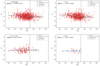 |
Fig. 1. Top-left: Spectroscopic β as a function of the absolute magnitude, MUV, for the entire sample (red points) in the redshift range between z = 4 and z = 14. The other three panels show the relation in redshift bins (z < 6.5, 6.5 < z < 8.5, z > 8.5). The best-fit linear relation for all the individual galaxies is shown with a solid orange line, while the best fit to the median points in bins of MUV (blue crosses) is indicated by a blue solid line. The dotted line shows the MUV = −18.5 limit. In the top-left corner of each panel, we highlight the slope of the best-fit relation. |
 (1)
(1)
A similar result is obtained when fitting a linear relation to the median β in different MUV bins. The negative, albeit shallow, slope of this relation is likely a consequence of the lower dust content and younger ages of intrinsically fainter galaxies, as noted in previous studies (e.g., Bouwens et al. 2012). It may also reflect the well-established mass-metallicity relation observed across a broad range of redshifts (e.g., Tremonti et al. 2004; Maiolino et al. 2008). For example, Calabrò et al. (2021) found a similar slope of −0.07 ± 0.03 by deriving β from photometry in the same wavelength range used in this study, based on the 572 galaxies at lower redshifts (2 < z < 5) and higher UV luminosities (−22 < MUV < −19.5) observed in the VANDELS spectroscopic survey.
To compare our results with recent JWST studies, we further analyzed the δβ/δMUV in redshift intervals. We derived a more negative slope at z < 6.5 (−0.11 ± 0.02) and a slope consistent with 0 in the two intervals 6.5 < z < 8.5 and z > 8.5, as shown in Fig. 2. In the top-right and bottoms panels of Fig. 1, we show the fits to the data points that produced the slope values δβ/δMUV presented in Fig. 2. This would indicate a flattening of the β versus MUV relation at higher redshifts.
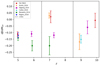 |
Fig. 2. Slope of the β vs. MUV relation in three different redshift bins spanning the range covered by our analysis. |
However, a similar result was suggested by Topping et al. (2024), who used a photometric sample and likewise found a flattening of the slope at higher redshifts, with a δβ/δMUV consistent with our result at 8.5 < z < 12. We note that while we agree with their median value at both the low- and high-redshift ends, our relation remains flat in the intermediate redshift range (approximately 6.5 < z < 8.5), where they instead find a negative slope. This difference may be due to the nonidentical redshift ranges considered in the two studies, resulting from different sample selections. In contrast, we find an opposite trend compared to Austin et al. (2024): their δβ/δMUV relation is flat in the intermediate redshift range (in agreement with ours) but becomes substantially steeper at z > 8.5. Similarly, Cullen et al. (2024) also find a steep negative relation at the significantly high-redshift end (z ∼ 9). We also compare our results with the pre-JWST studies by Rogers et al. (2014) and Bouwens et al. (2014), finding that our z < 6.5 value of δβ/δMUV agrees with theirs at z ∼ 5. However, the two additional values estimated by Bouwens et al. (2014) at z ∼ 5.9 and z ∼ 7 are steeper than ours, albeit with larger uncertainties.
Overall, Fig. 2 suggests that there is a large scatter in the derived δβ/δMUV, and reaching agreement among different studies remains difficult. This is likely due to a combination of different factors, including the use of different methods (spectroscopic slopes vs. photometric slopes), sample selection, and wavelength range employed for the derivation of the β slope.
A possible reason for the flattening of the β–MUV relation might be the absence of faint sources from the higher redshift samples due to the incompleteness of our sample. In Appendix A, we show that our spectroscopic sample is representative of the parent photometric sample down to a magnitude MUV, limit = −18.5 in the entire redshift range analyzed here. Another possible contribution to the observed trends is the reduced dynamical range of MUV at the highest redshifts, which decreases by a factor of ∼2 for z > 8.5 compared to the full sample. To investigate these effects on the evolution of the β versus MUV relation derived in this work, we considered the smaller subset with MUV < MUV, limit and repeated the fitting procedure over the entire redshift range as well as separately in the two lowest redshift bins (z < 6.5 and 6.5 < z < 8.5). As a result, we find a less negative slope for both the whole sample (the new slope is (δβ/δMUV)new = −0.03 ± 0.02) and the lowest redshift bin (−0.09 ± 0.03 at z < 6.5). These values remain consistent with the previous estimates within 1σ and are still significantly lower than 0. In the intermediate redshift bin, we also obtain a slope (0.03 ± 0.05) consistent with the previous value. Overall, this shows that selection effects play a minor role and cannot fully explain the flattening of the β versus MUV relation at z > 6.5.
3.2. Redshift evolution
To follow, we investigated how the UV slopes of galaxies evolve at z > 4. To this end, we plotted β as a function of the spectroscopic redshift for the entire sample. Our results are shown in Fig. 3. We can see that the UV slope of galaxies becomes bluer on average from z = 4 to z ≃ 10, with median β values decreasing by 0.3 from –1.9 at z ∼ 4.5 to –2.1 at z ∼ 10. A global linear fit yields
 (2)
(2)
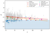 |
Fig. 3. Redshift evolution of the spectroscopic β from z = 4 to z = 14. The best-fit linear relation of all the individual galaxies (gray points) is shown with a red solid line, while the best-fit to the medium points in the redshift bins (red circles) is displayed with a red dashed line. Average UV slopes from the literature are also shown for comparison. The blue points are the XBGs studied in Sect. 4. |
We also performed a linear fit to the median β values calculated in the redshift bins 4–5, 5–6, 6–8, and 8–14, yielding a slightly shallower relation as given by
 (3)
(3)
A similar slope and intercept are obtained when considering the UV slopes estimated with the Monte Carlo fit method. An evolution toward bluer UV colors at higher redshifts is not only physically significant, but also expected, as galaxies become progressively metal- and dust-poor at earlier cosmic times. Prior to JWST, this trend had been observed up to z ≈ 8 (e.g., Bouwens et al. 2014).
The slope of our β–z relation is consistent with recent results based on photometric UV slopes, including those reported by Austin et al. (2024) and Roberts-Borsani et al. (2024). The consistency is slightly improved for the steeper linear fit obtained when considering all the individual points. The normalization of our relation agrees with that obtained by Austin et al. (2024) within a 1σ uncertainty, although a small positive offset (∼ + 0.1) emerges toward higher redshifts, where our statistics are poorer. This overall consistency suggests that no significant biases exist between spectroscopic and photometric-based UV slope estimates once proper correction factors for emission lines are taken into account in the latter method. A larger offset of ∼ + 0.5 is found with the relation from Roberts-Borsani et al. (2024), with our slopes being systematically redder. This is likely due to the different wavelength range (1600 Å < λrest < 2800 Å) used for fitting the UV slope in their work. Including the bluest portion of our fitted range may contribute to a slight reddening of the overall shape of the UV continuum, an effect which we will discuss further in Sect. 3.3.
In the redshift range between 4 and 7, we obtain slightly redder UV slopes on average (by ∼0.2) compared to Nanayakkara et al. (2023), although the results are consistent within the uncertainties, and we find a similar slope for the β–z relation. Their work also uses only photometric data to compute the UV slope from the best-fit EAzY SEDs in the 1400–2000 Å range, which is again redder than our range. Finally, we compare our results to the analysis of Cullen et al. (2024), which is focused on the highest redshift range (z > 8) and also employs photometric data. However, they include IGM modeling in their derivation, as they also use filters encompassing the Lyman break. Our median β are consistent with their results only at z ∼ 9.5 − 10.5, while being bluer at z = 8.5 and redder at z > 11. Their overall trend suggests a faster evolution of β with redshift. The limited redshift coverage of these latter two studies does not allow us to make a global comparison from z = 4 to z ∼ 10.
We also checked for possible variations in the slope of the β − z relation as a function of the UV magnitude of galaxies, as suggested by recent studies (e.g., Topping et al. 2024). For this reason, we split our sample into three different MUV bins (MUV < −19, −19 < MUV < −18, −18 < MUV < −17). We find no significant variations in the slope of the best-fit relation across the entire redshift range in galaxies down to MUV = −18, in agreement with the results of Austin et al. (2024). We are not able to constrain the full redshift evolution for the faintest magnitude bin since, for reasons already stated in the previous section, we lack sources with MUV fainter than –18 at z > 8.
To conclude, our analysis suggests that the spectroscopic UV β follows a mild but significant decrease at higher redshifts, which is similar to the result obtained with the photometric β. This trend is consistent with the scenario where galaxies become increasingly more metal- and dust-poor toward earlier cosmic epochs, as already discussed in several pre-JWST studies (e.g., Dunlop et al. 2013; Finkelstein et al. 2012; Bouwens et al. 2012; Wilkins et al. 2016).
3.3. Evidence for Lyman α damping wing
During the EoR, Lyα photons from galaxies are absorbed by neutral hydrogen present in the surrounding IGM. At high redshift, the line is so saturated that even photons emitted redward of the Lyα resonance can suffer significant absorption from the strong damping wings of that transition, resulting in a characteristic shape of the spectrum immediately redward of the Lyα emission and up to 100 Å from resonance. The most widely used prescription of the Lyα damping wing (DW) is shown in Miralda-Escudé (1998). This model assumes that the IGM has a constant (volume-averaged) neutral hydrogen fraction, xHI, between the source redshift, zgal, and at the end of reionization, zRe. In contrast, recent comparisons to theorized damping wing profiles assume a more realistic patchy reionization process (e.g., Keating et al. 2024).
Before JWST, DW features in the EoR were typically searched for in bright QSO spectra, as their intense flux allows us to obtain high S/N spectra (Mortlock et al. 2011; Bañados et al. 2018). NIRSpec-PRISM observations allow us to likewise obtain comparable high S/N spectra for galaxies. These are much more numerous and, thus, probe less biased regions of the Universe. Several studies attempted measurements of the Lyα DW to constrain the reionization process (e.g., Umeda et al. 2024; Witstok et al. 2025). However, the additional effect of damped Lyman α (DLA) systems with high column densities of neutral hydrogen NHI > 2 ⋅ 1020 cm−2 (Lanzetta 2000) from dense gas clouds associated with the galaxies must also be considered. DLAs have been observed at high redshift both in quasar (Totani et al. 2006) and galaxy spectra (Heintz et al. 2025). This component should be added to the IGM effect, complicating the derivation of the true IGM opacity (e.g., Park et al. 2025).
The opacity due to DLA can be distinguished from the IGM effect thanks to different wavelength dependence. This nevertheless requires high-resolution spectra that typically do not reach a high S/N in the continuum. We approached the problem by studying the average UV β slopes of our large sample of galaxies as a function of wavelength and redshift. Specifically, we recalculated the slopes excluding the region of the spectra that could potentially be affected by flux reduction due to the DW effects of the IGM and/or the DLA systems, and, thus, could lead to redder-than-expected UV-slopes. We derived βDW as the slope calculated using all the Calzetti et al. (1994) windows except the first two, starting at 1340 Å instead of 1270 Å. We then focused on the difference, β − βDW. If the flux in the range 1270 Å < λ < 1340 Å is reduced due to the Lyα DW, βDW becomes bluer than β, resulting in a positive difference for β − βDW. We note that this analysis assumes the intrinsic spectra are perfectly described by a power law in this range, which may not be true (Bouwens et al. 2012). However, our primary interest lies in studying the average β − βDW as a function of redshift, to assess whether there is substantial evolution of this difference around the EoR – a trend that could likely be attributed to increasingly neutral IGM rather than other effects. Since the presence of DLA systems may also depend on galaxy brightness, we further restrict our analysis to sources with MUV < −18.6, above which we have essentially no statistics at higher redshifts. This reduces the total sample to 407 galaxies.
In Fig. 4, we show our results. For most sources, the β − βDW is positive, indicating that using a longer wavelength cutoff yields slightly bluer slopes. This is consistent with expectations and with our discussions in the previous section comparing our results to other analyses. For the entire sample, we find ⟨β − βDW⟩tot = 0.042 ± 0.002.
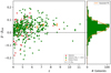 |
Fig. 4. Redshift evolution of the function β − βDW. All galaxies reported in the plot have S/N > 5. Furthermore, the 407 green galaxies shown satisfy the condition MUV < −18.6. The orange points represent the median values of the green points in redshift bins. On the right panel, a histogram of the green points is shown, fit by a Gaussian function with μ = 0.042 ± 0.002 and σ = 0.038 ± 0.001. |
Dividing our sample in redshift bins between 4 < z < 6, the median value is approximately ⟨β − βDW⟩4 < z < 6 = 0.039 ± 0.005, while for z > 7.5 the median value is ⟨β − βDW⟩z > 7.5 = 0.062 ± 0.010. This difference is significant and could be attributed to the increasing presence of neutral hydrogen in the IGM, generally affecting galaxies at high redshift. We also note that almost all galaxies at z > 7.5 have only positive β − βDW. To determine whether this apparent increase at z = 7.5 is due to a physical effect or simply to lower statistics at high redshift (where we only have 22 galaxies), we performed a two-sample Kolmogorov-Smirnov (KS) test. The null hypothesis is that the distributions of β − βDW at low and high redshift are identical. We obtain a p-value of 0.044. If we choose a 2σ confidence level, a p-value less than 0.05 would reject the null hypothesis. This means that the data would not be drawn from the same distribution and would have a higher value of β − βDW above z ≃ 7.5. This could indicate that, at this high redshift, the extra signal in the DW is indeed due to the effect of the neutral IGM, assuming that the effect of the DLA systems does not evolve with the redshift. However, the effect is significantly small; therefore, spectra with higher resolution and significantly high S/N are required to study this effect, as also discussed by Park et al. (2025).
4. Extremely blue galaxies
4.1. Selection
We define XBGs as those systems with a UV spectral slope lower than –2.6. This threshold corresponds to the theoretical lower limit expected for young stellar populations in case of zero dust attenuation and full contribution from the nebular continuum – assuming that no ionizing photons escape from the galaxy (Robertson et al. 2010; Cullen et al. 2017; Topping et al. 2022; Reddy et al. 2018). This limit is also in agreement with observations of dust-poor, local, star-forming galaxies (Chisholm et al. 2022). In our sample, we identify 44 XBGs with β < −2.6. Among these, 15 sources have β slopes lower than –2.6 within their 1σ uncertainties. We also assembled a control sample of redder galaxies (hereafter dubbed red galaxies) with β between –1.8 and –1.5. We selected this subset as follows: for each XBG, we randomly selected one red galaxy with a similar redshift (within ±0.5) and a similar MUV (within ±0.2), in order to exclude biases due to β evolving with redshift and UV magnitude. This yields a redshift- and MUV-matched subset of 44 red galaxies.
4.2. Comparing the properties of XBGs and red galaxies through a spectral stacking analysis
To investigate which mechanisms could play a role in producing blue UV slopes, we explored how the global physical properties of XBGs differ from those of red galaxies. Since faint optical and UV rest-frame lines (i.e., [O II] λ3727 Å, [Ne III] λ3868 Å, He IIλ1640 Å, C IIIλλ1907 − 1909) are not detected for a significant fraction of our sample, we performed a spectral stack for the subsets.
For the stacking procedure, we adopted the same methodology used in our previous studies (Calabrò et al. 2022a,b, 2023). In detail, we first converted all the spectra of XBGs and red galaxies to rest-frame using their spectroscopic redshift. We then normalized them to the median flux calculated between 2500 and 3000 Å rest-frame and resampled them to a common grid of 2.4 Å per pixel, corresponding to approximately 1/3 of the resolution element from 800 to 7000 Å rest-frame. Lastly, for each pixel, we median averaged all the fluxes after a 3σ clipping rejection. The stacked noise spectrum was instead derived with a bootstrap resampling procedure with 1000 iterations. The final stacks for the control sample and the XBGs are shown in Figs. 5 and 6, respectively.
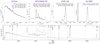 |
Fig. 5. Spectral stacks of the red galaxy population, as defined in the text, between 1150 and 6700 Å rest-frame. The position of several UV and optical lines is indicated with vertical gray dashed lines. The same panel shows the fit for deriving the optical break. On top of the stack the fit of the UV lines, the [O II] λ3727 Å+[Ne III] λ3868 Å+Hδ lines, the [O III] λ5007 Å+Hβ triplet, and the Hα+[S II] λλ6717 − 6731 lines, as detailed in the text, are shown. The full spectrum is indicated with a blue solid line. The black spectrum is the fitted region, and the red curve represents the best-fit profile. In each panel, fluxes, 1σ uncertainties, and underlying continuum are also indicated for each of the fitted lines highlighted with thin vertical dashed lines. |
To obtain quantitative information on the nebular and stellar properties of the two populations, we measured the fluxes and the equivalent width (EW) of the most relevant emission lines detected in the entire UV and optical range, following a well-tested approach from our previous studies. In short, we fit a Gaussian profile with an underlying linear continuum in the Fλ-wavelength parameter space, within a window of ±3000 km/s from the line peak wavelength. In the rest-frame optical, we fit together the [O III] λ5007 Å+Hβ triplet, and the following four lines – [O II] λ3727 Å, [Ne III] λ3868 Å, [Ne III] λ3967 Å, and Hδ – as they are significantly close in wavelength. To avoid the Balmer break rightward of [O II], the underlying stellar continuum was mainly estimated from the redder part of the spectrum. Given the low spectral resolution of the prism configuration, we fit the Hα+[S II] λλ6717 − 6731 doublet with two Gaussians. We then reduced the flux of Hα by a factor of 1.05, considering the average [N II]/Hα ratio estimated from grating spectra for star-forming galaxies at similar redshifts by Shapley et al. (2023). Lastly, in the rest-frame UV, we simultaneously fit the N IVλ1488 Å, C IVλ1549 Å, He IIλ1640 Å, [O III] λ1663 Å, N IIIλ1750 Å, and C IIIλ1908 Å lines on top of a power-law stellar continuum, as this approach is more robust compared to the fit of individual lines when the resolution is low (Calabro et al., in prep.). We also assumed a common redshift for the lines and a common intrinsic line width. We computed the rest-frame EW of the lines and the Hα/Hβ ratio, from which we estimated the dust attenuation AV by assuming a Calzetti et al. (2000) attenuation law. From the line fluxes, we computed the following (attenuation corrected) line ratio indices probing the average physical conditions in the ISM:
-
log([O II]λλ3726,3729/Hβ) (R2),
-
log([O III]λ5007/Hβ) (R3),
-
log(([O III]λλ4959,5007 + [O II]λλ3726,3729)/Hβ) (R23),
-
log(([O III]λλ4959,5007 / [O II]λλ3726,3729) (O32),
-
log(Ne III]λ3869 / [O II]λλ3726,3729) (Ne3O2), and
-
log([O III]λλ4959,5007 / [O III]λλ1661,1666) (O3).
We also measured the Balmer break (hereafter dubbed “optical break”), which indicates the age of underlying stellar populations. We adopted the definition of Roberts-Borsani et al. (2024), who compared the continuum estimated in the wavelength regions between λrest = 3500 and 3630 Å (leftward of the break) and = 4160 and 4290 Å (rightward of the break), to avoid contribution from strong emission lines in our low-resolution spectra and mitigate the impact of noise. From the two continuum measurements, we lastly computed the Fν, 4200/Fν, 3500 ratio.
The results of all these measurements are summarized in Table 2 for the XBGs and the red galaxies’ stacks. In both cases, we detect the following rest-frame optical lines: [O II] λ3727 Å, [Ne III] λ3868 Å, Hγ, Hβ, [O III] λ5007 Å, Hα, and C IIIλλ1907 − 1909 in the UV rest-frame. In the XBG stack, we additionally detect the He IIλ1640 Å and [O III] λ1663 Å lines. We also tentatively detect the NIV]1488 Å line in the ultrablue stack, but given its low significance level (S/N < 3), we do not discuss it in detail.
Main spectral indices and physical properties of XBGs and red galaxies.
Focusing on stellar population properties, we find that the XBGs have an optical break Fν, 4200/Fν, 3500 that is ∼15% smaller than in the red galaxy sample. This value indicates the substantially younger ages of the emitting stars. The EW of the He IIλ1640 Å line (EW ≃ 4 Å) detected in the stack of XBGs could also indicate the presence of Wolf-Rayet stars (WR, Schaerer 1996; Shirazi & Brinchmann 2012), massive interacting binary stars (Steidel et al. 2016; Nakajima et al. 2018), or significantly massive stars with masses > 100 M⊙ (VMS, Schaerer et al. 2025) as primary ionization sources. These are expected to contribute significantly during the first 10 Myrs of star formation. This further suggests that the two populations may differ substantially in stellar age. In principle, higher resolution spectra could help to distinguish between the WR and VMS scenarios, as broad He II lines with FWHMvelocity > 1000 km/s are expected in the former case. We also find that XBGs, on average, have lower stellar masses (average log M*/M⊙ = 8.0) than red galaxies by ∼0.6 dex, as they are less evolved systems.
The Balmer decrement is different between these two populations. Although both are above the case B recombination limit of 2.86, the XBGs have a lower Hα/Hβ ratio than the red subset. Converting Hα/Hβ to a gas phase dust attenuation, AV, and assuming the attenuation law of Calzetti et al. (2000), the XBGs and red galaxies have an AV of 0.2 ± 0.2 and 0.7 ± 0.2 mag, respectively. If we further analyze the gas properties, the XBGs have on average a higher O32 and a higher Ne3O2 index by ∼0.1 dex and ∼0.3 dex (respectively), indicating stronger ionizing conditions in these galaxies compared to red galaxies. These values suggest that the ionization parameter of both subsets is between log(U) ∼ − 2 and –2.5, according to the photoionization models presented in Calabrò et al. (2023). A more quantitative assessment using the calibration of Papovich et al. (2022) on the O32 index yields a log(U) = − 2.11 ± 0.03 for the XBGs, ∼0.1 dex higher than in the red galaxies. Lastly, we measure a slightly higher EW(C III]) for the red galaxies, although both measurements are consistent with the EW(C III]) of typical high-z star-forming galaxies (see e.g., Amorín et al. 2017; Nakajima et al. 2018; Llerena et al. 2022), as well as with the average range measured recently with JWST data for the global population of star-forming galaxies at z ∼ 5 (Roberts-Borsani et al. 2024).
The line indices presented in Table 2 can be used to infer the gas-phase metallicity, Zgas, of the galaxies. Using the full set of five spectral indices – R2, R3, R23, O32, and Ne3O2 – we calculated Zgas for the two spectral stacks, applying the strong-line calibrations of Sanders et al. (2024). These calibrations are based on a large subset of galaxies from z = 2 to z = 9, covering a similar stellar mass and star formation rates as our high-redshift galaxies, and anchored to the electron temperature (Te) method.
We find that, regardless of the index, Zgas of XBGs is always lower than Zgas in red galaxies. Calculating an error-weighted average of the metallicities estimated with all the five indices yields Zgas ∼ 10% Z⊙ in XBGs and ∼16% in red galaxies. In the stack of XBGs, we also detect the [O III] λ1663 Å line and, through the direct Te method, obtain a metallicity of 9 ± 1% Z⊙ in line with the strong-line method. These results indicate a significant difference in metallicity, at > 5σ significance, between the two subsets, with XBGs being more metal-poor than red galaxies.
The difference in metallicity between XBGs and red galaxies reflects the strong correlation observed between the UV slope, the gas-phase, and the stellar metallicity of star-forming galaxies at lower redshifts (Shivaei et al. 2020; Calabrò et al. 2021). Since the UV slopes are primarily regulated by the amount of dust attenuating the stellar intrinsic spectrum, this again suggests that XBGs are chemically young systems, less enriched in dust and metals compared to more evolved, red galaxies.
Overall, our findings suggest that XBGs have younger stellar populations, stronger ionization fields, lower dust attenuation, and lower metallicity compared to red galaxies. It is worth noting that, despite their extreme β values, XBGs do not contain pristine gas with zero metallicity. Rather, their ISM is already enriched at almost 10% solar. Using the SED models from Fig. 2 of Topping et al. (2022), assuming a stellar metallicity of 10% solar and, more conservatively, down to a Z = 1% Z⊙ to account for the possible rescaling between the gas-phase and stellar metallicity, we note that – even though stellar populations with significantly low metallicities and young ages have bluer intrinsic spectra – metallicity or age alone cannot explain β values < − 2.6. This analysis suggests that the only factor capable of producing UV spectra significantly bluer than β ≃ −2.6 is a lower contribution from the nebular continuum emission and, therefore, implies a significant leakage of ionizing radiation. We explore this scenario in the next subsection.
4.3. The origins of the very blue UV spectral slopes
Previous studies have shown that reducing the contribution of the nebular continuum emission is a viable way to obtain UV slopes bluer than –2.6. This can occur if a fraction of the stellar continuum emission does not ionize the surrounding ISM but instead is able to propagate freely outside of the galaxy. One way to test this scenario is by calculating the escape fraction of Lyman continuum radiation (fesc), for the XBGs and the red galaxies populations to assess if they are different.
At z > 4, it is impossible to directly detect the Lyman continuum emission due to IGM opacity. Several studies nevertheless show that fesc can be estimated indirectly. The simplest method is to directly apply the relation between β and fesc derived by Chisholm et al. (2022), as previously done by Cullen et al. (2024); this would imply fesc > 0.19 for all the XBGs and a median fesc = 0.013 for the red galaxies. However, this relation shows a really large scatter when applied to Low-redshift Lyman Continuum Survey leakers. For this reason, alternative methods developed, based on a combination of several indirect indicators (Jaskot et al. 2024; Mascia et al. 2023; Choustikov et al. 2024), give more robust estimates for intermediate redshift leakers (Jaskot et al. 2024; Mascia et al. 2025). We applied the Cox proportional hazards models of Jaskot et al. (2024), which are based on a survival analysis technique and recalibrated by Mascia et al. (2025) on Low-redshift Lyman Continuum Survey galaxies that are analogs of EoR sources. Specifically, we applied the “ELG-O32” model which uses a combination of the stellar mass, the stellar attenuation AV, stellar, the UV magnitude MUV, and the O32 index, defined as log([O III]5007/[O II]3727), to indirectly infer the escape fraction of ionizing photons. The stellar mass, MUV, and the stellar attenuation AV, stellar were derived from fitting stellar population templates with nebular contribution to the available multiwavelength photometry from Merlin et al. (2024), using the code zphot.exe (Fontana et al. 2000). The O32 indices were measured directly from the individual spectra and corrected for dust attenuation using the Hα/Hβ ratio, or, above the redshift where Hα is not covered by NIRSpec, using the nebular attenuation AV, neb = AV, stellar/0.44. If [O II]3727 was not detected, we calculated a 1σ lower limit for fesc.
We compare the distributions of fesc of the XBGs and red galaxy populations in Fig. 7-left. Overall, we find that both distributions are non-Gaussian, with a bulk of galaxies having significantly low escape fractions (< 0.01) and with a tail of galaxies with higher fesc similar to the results of previous works on galaxies at similar redshift (Mascia et al. 2023, 2024). A similar exponential-like distribution of fesc has been inferred by Kreilgaard et al. (2024) using a direct probe of the Lyman continuum flux at z = 3.5. The XBG population has an average fesc = 0.08 that is ∼8 times higher than that of the red galaxy population and attains a much higher maximum escape fraction (0.44 compared to 0.12). A KS test confirms that the XBG and red galaxy subsets are likely taken from two different underlying distributions (KS-statistics = 0.45, p-value = 0.001). We also compared the cumulative distribution functions (CDF) of the two XBGs and the red galaxies (Fig. 7-right). Using these CDFs, we additionally performed a Mann-Whitney U test, which yielded a p-value of 7 × 10⁻⁵, further indicating that the difference between the distributions is statistically significant.
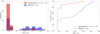 |
Fig. 7. Left: Histogram distribution of the escape fractions (estimated indirectly, as explained in the text, and in logarithmic scale) for the subsets of XBGs (blue bars) and red galaxies (red bars), matched in redshift and MUV to the XBGs. Right: Cumulative distribution functions of log10fesc for XBGs and red galaxies (blue dashed and red solid line, respectively). |
This suggests that the higher escape fraction of Lyman continuum radiation could be a reason for the extremely blue slopes in some the XBGs, especially considering that for more than half of the blue sources, the inferred fesc are lower limits. It is also important to acknowledge that, since the majority of sources with β < −2.6 are within 1σ, it is likely that some of those with fesc = 0 have true UV slopes that are actually much redder. However, as shown by Topping et al. (2022), model predictions indicate that only extreme fesc values yield the β as blue as –3, whereas only a few of our XBGs exhibit inferred fesc > 0.1.
Alternatively, the blue sources might be caught in a peculiar moment of cessation of star formation shortly after a burst, as proposed by Topping et al. (2024). In this case, the ionizing photon production and the resulting nebular continuum strength fall, and we observe purely stellar continuum in the UV. With such young stellar ages, the UV slope can be significantly blue. Indeed, JWST studies provide evidence for bursty star formation histories at the EoR (Asada et al. 2024; Endsley et al. 2024). We will perform a detailed spectro-photometric analysis in a future study.
5. Summary
In this work we analyzed a large sample of 726 galaxies selected from a mixture of JWST ERS, GTO, and GO observational programs with z > 4 and boasting spectroscopic data obtained with the low-resolution (R ∼ 30 − 300) PRISM/CLEAR NIRSpec configuration. We determined their UV continuum slopes β with the main goal of studying the evolution of the average properties of galaxies over a large cosmic epoch. We also identified a subset of sources showing spectral slopes bluer than –2.6, which, in case of no dust attenuation, is bluer than the lower limit that can be reached with stellar plus nebular continuum emission. We analyzed them both individually and through spectral stacking to uncover the physical origin of their extremely blue slopes.
We summarize the main results of our work as follows:
-
We find a shallow dependence of β on MUV (best-fit slope of −0.055 ± 0.017) for the entire sample. We also find that the β-MUV relation tends to flatten toward higher redshifts, going from a slope of δβ/δMUV ∼ −0.1 at z < 6.5 to ∼0 at z > 6.5.
-
The average β slopes follow a mild but significant evolution with redshift, with galaxies becoming bluer toward earlier cosmic epochs (δβ/δz = −0.075). These findings are consistent with the results obtained for galaxies with similar redshifts and UV luminosities as well as UV slopes measured from photometric data.
-
We analyzed the Lyα DW in the spectra, which we know is due to a combination of increasing neutral hydrogen present in the IGM as well as from the DLA systems associated with the galaxies. While the former effect should only appear when the IGM is significantly neutral (z > 7), the latter should be redshift independent in an MUV limited sample. We find a small but significant effect on the β slope at z > 7.5 that suggests an increase in the neutral IGM content. This is, however, difficult to quantify with current low-resolution data.
-
We obtained a stacked spectrum of the galaxies with extremely blue UV slopes (β < −2.6), and compared the average properties determined from the detected emission lines to an analogous spectral stack of a sample of red sources (−1.8 < β < −1.5) matched in MUV and redshift. We find that XBGs have a higher ionization parameter, lower (although not pristine) metallicity, and younger ages than redder galaxies. However, these properties alone cannot explain their extreme β values.
-
Using the most solid indirect predictors of the Lyman continuum escape recently developed (Jaskot et al. 2024; Mascia et al. 2025), we find that the escape fraction fesc may be > 10% in a large fraction of the XBGs, contrary to what has been inferred for red galaxies with the same MUV and redshift. The reduction of the nebular continuum, resulting from a large leakage of ionizing photons, would therefore account for the blue spectral slopes. However, some XBGs also have significantly low escape fractions, suggesting that other physical mechanisms, such as a bursty star formation history, must also play a role.
Future large spectroscopic surveys, such as CAPERS (JWST GO 6838), will significantly increase the number of galaxies with spectroscopic follow-up in the reionization epoch. This will allow us to constrain more robustly the evolution of beta with redshift, and the slope of the β–MUV relation, testing also the role of other physical properties in those relations. Deeper and higher resolution spectra in the UV rest-frame will, instead, help us to better constrain the Lyα DW profile and to distinguish the different contributions from DLA and IGM absorption, aided by the latest models and radiative transfer cosmological simulations.
Acknowledgments
We acknowledges support from the INAF Large Grant for Extragalactic Surveys with JWST and from the PRIN 2022 MUR project 2022CB3PJ3 – First Light And Galaxy aSsembly (FLAGS) funded by the European Union – Next Generation EU. PS acknowledges INAF Mini Grant 2022 “The evolution of passive galaxies through cosmic time”. Part of the research activities described in this paper were carried out with the contribution of the Next Generation EU funds within the National Recovery and Resilience Plan (PNRR), Mission 4 – Education and Research, Component 2 – From Research to Business (M4C2), Investment Line 3.1 – Strengthening and creation of Research Infrastructures, Project IR0000034 – “STILES – Strengthening the Italian Leadership in ELT and SKA”. RA acknowledges support of Grant project PID2023-147386NB-I00 funded by MICIU/AEI/10.13039/501100011033 and by ERDF/EU, and the Severo Ochoa grant CEX2021-001131-S funded by MCIN/AEI/10.13039/50110001103.
References
- Adamo, A., Atek, H., Bagley, M. B., et al. 2024, arXiv e-prints [arXiv:2405.21054] [Google Scholar]
- Amorín, R., Fontana, A., Pérez-Montero, E., et al. 2017, NatAs, 1, 0052 [Google Scholar]
- Asada, Y., Sawicki, M., Abraham, R., et al. 2024, MNRAS, 527, 11372 [Google Scholar]
- Asplund, M., Grevesse, N., Sauval, A. J., et al. 2009, ARA&A, 47, 481 [Google Scholar]
- Atek, H., Shuntov, M., Furtak, L. J., et al. 2023, MNRAS, 519, 1201 [Google Scholar]
- Austin, D., Adams, N., Conselice, C. J., et al. 2023, ApJ, 952, L7 [NASA ADS] [CrossRef] [Google Scholar]
- Austin, D., Conselice, C. J., Adams, N. J., et al. 2024, ApJ, submitted [arXiv:2404.10751] [Google Scholar]
- Bañados, E., Venemans, B. P., Mazzucchelli, C., et al. 2018, Nature, 553, 473 [Google Scholar]
- Bouwens, R. J., Illingworth, G. D., Oesch, P. A., et al. 2012, ApJ, 754, 83 [Google Scholar]
- Bouwens, R. J., Illingworth, G. D., Oesch, P. A., et al. 2014, ApJ, 793, 115 [Google Scholar]
- Brammer, G. 2023, https://doi.org/10.5281/zenodo.8370018 [Google Scholar]
- Calabrò, A., Castellano, M., Pentericci, L., et al. 2021, A&A, 646, A39 [EDP Sciences] [Google Scholar]
- Calabrò, A., Guaita, L., Pentericci, L., et al. 2022a, A&A, 664, A75 [NASA ADS] [CrossRef] [EDP Sciences] [Google Scholar]
- Calabrò, A., Pentericci, L., Talia, M., et al. 2022b, A&A, 667, A117 [NASA ADS] [CrossRef] [EDP Sciences] [Google Scholar]
- Calabrò, A., Pentericci, L., Feltre, A., et al. 2023, A&A, 679, A80 [NASA ADS] [CrossRef] [EDP Sciences] [Google Scholar]
- Calabrò, A., Pentericci, L., Santini, P., et al. 2024, A&A, 690, A290 [NASA ADS] [CrossRef] [EDP Sciences] [Google Scholar]
- Calzetti, D., Kinney, A. L., & Storchi-Bergmann, T. 1994, ApJ, 429, 582 [Google Scholar]
- Calzetti, D., Armus, L., Bohlin, R. C., et al. 2000, ApJ, 533, 682 [NASA ADS] [CrossRef] [Google Scholar]
- Castellano, M., Fontana, A., Grazian, A., et al. 2012, A&A, 540, A39 [NASA ADS] [CrossRef] [EDP Sciences] [Google Scholar]
- Chabrier, G. 2003, PASP, 115, 763 [Google Scholar]
- Chisholm, J., Saldana-Lopez, A., Flury, S., et al. 2022, MNRAS, 517, 5104 [CrossRef] [Google Scholar]
- Choustikov, N., Katz, H., Saxena, A., et al. 2024, MNRAS, 529, 3751 [NASA ADS] [CrossRef] [Google Scholar]
- Cullen, F., McLure, R. J., Khochfar, S., et al. 2017, MNRAS, 470, 3006 [NASA ADS] [CrossRef] [Google Scholar]
- Cullen, F., McLure, R. J., McLeod, D. J., et al. 2023, MNRAS, 520, 14 [NASA ADS] [CrossRef] [Google Scholar]
- Cullen, F., McLeod, D. J., McLure, R. J., et al. 2024, MNRAS, 531, 997 [NASA ADS] [CrossRef] [Google Scholar]
- Curti, M., D’Eugenio, F., Carniani, S., et al. 2023, MNRAS, 518, 425 [Google Scholar]
- D’Eugenio, F., Cameron, A. J., Scholtz, J., et al. 2025, ApJS, 277, 4 [Google Scholar]
- Dunlop, J. S., Rogers, A. B., McLure, R. J., et al. 2013, MNRAS, 432, 3520 [NASA ADS] [CrossRef] [Google Scholar]
- Eisenstein, D. J., Willott, C., Alberts, S., et al. 2023, ApJS, submitted [arXiv:2306.02465] [Google Scholar]
- Endsley, R., Stark, D. P., Whitler, L., et al. 2024, MNRAS, 533, 1111 [NASA ADS] [CrossRef] [Google Scholar]
- Finkelstein, S. L., Papovich, C., Salmon, B., et al. 2012, ApJ, 756, 164 [NASA ADS] [CrossRef] [Google Scholar]
- Finkelstein, S. L., Bagley, M. B., Ferguson, H. C., et al. 2023, ApJ, 946, L13 [NASA ADS] [CrossRef] [Google Scholar]
- Fontana, A., D’Odorico, S., Poli, F., et al. 2000, AJ, 120, 2206 [NASA ADS] [CrossRef] [Google Scholar]
- Giavalisco, M., Ferguson, H. C., Koekemoer, A. M., et al. 2004, ApJ, 600, L93 [NASA ADS] [CrossRef] [Google Scholar]
- Goulding, A. D., Greene, J. E., Setton, D. J., et al. 2023, ApJ, 955, L24 [NASA ADS] [CrossRef] [Google Scholar]
- Greene, O., Falcone, J., Marinelli, M., et al. 2023, A&A, 241, 408.04 [Google Scholar]
- Grogin, N. A., Kocevski, D. D., Faber, S. M., et al. 2011, ApJS, 197, 35 [NASA ADS] [CrossRef] [Google Scholar]
- Harikane, Y., Zhang, Y., Nakajima, K., et al. 2023, ApJ, 959, 39 [NASA ADS] [CrossRef] [Google Scholar]
- Hathi, N. P., Cohen, S. H., Ryan, R. E., et al. 2013, ApJ, 765, 88 [Google Scholar]
- Hathi, N. P., Le Fèvre, O., Ilbert, O., et al. 2016, A&A, 588, A26 [NASA ADS] [CrossRef] [EDP Sciences] [Google Scholar]
- Heintz, K. E., Brammer, G. B., Watson, D., et al. 2025, A&A, 693, A60 [Google Scholar]
- Jakobsen, P., Ferruit, P., Alves de Oliveira, C., et al. 2022, A&A, 661, A80 [NASA ADS] [CrossRef] [EDP Sciences] [Google Scholar]
- Jaskot, A. E., Silveyra, A. C., Plantinga, A., et al. 2024, ApJ, 973, 111 [NASA ADS] [CrossRef] [Google Scholar]
- Jones, G. C., Bunker, A. J., Saxena, A., et al. 2024, A&A, 683, A238 [NASA ADS] [CrossRef] [EDP Sciences] [Google Scholar]
- Keating, L. C., Bolton, J. S., Cullen, F., et al. 2024, MNRAS, 532, 1646 [Google Scholar]
- Kewley, L. J., Nicholls, D. C., & Sutherland, R. S. 2019, ARA&A, 57, 511 [Google Scholar]
- Kocevski, D. D., Onoue, M., Inayoshi, K., et al. 2023, ApJ, 954, L4 [NASA ADS] [CrossRef] [Google Scholar]
- Koekemoer, A. M., Faber, S. M., Ferguson, H. C., et al. 2011, ApJS, 197, 36 [NASA ADS] [CrossRef] [Google Scholar]
- Kreilgaard, K. C., Mason, C. A., Cullen, F., et al. 2024, A&A, 692, A57 [NASA ADS] [CrossRef] [EDP Sciences] [Google Scholar]
- Kurczynski, P., Gawiser, E., Rafelski, M., et al. 2014, ApJ, 793, L5 [Google Scholar]
- Lanzetta, K. 2000, in Encyclopedia of Astronomy and Astrophysics, ed. P. Murdin (Bristol: Institute of Physics Publishing), 2141 [Google Scholar]
- Larson, R. L., Finkelstein, S. L., Kocevski, D. D., et al. 2023, ApJ, 953, L29 [NASA ADS] [CrossRef] [Google Scholar]
- Llerena, M., Amorín, R., Cullen, F., et al. 2022, A&A, 659, A16 [NASA ADS] [CrossRef] [EDP Sciences] [Google Scholar]
- Llerena, M., Amorín, R., Pentericci, L., et al. 2024, A&A, 691, A59 [NASA ADS] [CrossRef] [EDP Sciences] [Google Scholar]
- Maiolino, R., Nagao, T., Grazian, A., et al. 2008, A&A, 488, 463 [NASA ADS] [CrossRef] [EDP Sciences] [Google Scholar]
- Mascia, S., Pentericci, L., Calabrò, A., et al. 2023, A&A, 672, A155 [NASA ADS] [CrossRef] [EDP Sciences] [Google Scholar]
- Mascia, S., Pentericci, L., Calabrò, A., et al. 2024, A&A, 685, A3 [NASA ADS] [CrossRef] [EDP Sciences] [Google Scholar]
- Mascia, S., Pentericci, L., Llerena, M., et al. 2025, A&A, submitted [arXiv:2501.08268] [Google Scholar]
- Mazzolari, G., Scholtz, J., Maiolino, R., et al. 2024, A&A, accepted [arXiv:2408.15615] [Google Scholar]
- Merlin, E., Santini, P., Paris, D., et al. 2024, A&A, 691, A240 [NASA ADS] [CrossRef] [EDP Sciences] [Google Scholar]
- Messa, M., Vanzella, E., Loiacono, F., et al. 2025, A&A, 694, A59 [NASA ADS] [CrossRef] [EDP Sciences] [Google Scholar]
- Meurer, G. R., Heckman, T. M., & Calzetti, D. 1999, ApJ, 521, 64 [Google Scholar]
- Miralda-Escudé, J. 1998, ApJ, 501, 15 [CrossRef] [Google Scholar]
- Morales, A. M., Finkelstein, S. L., Leung, G. C. K., et al. 2024, ApJ, 964, L24 [NASA ADS] [CrossRef] [Google Scholar]
- Mortlock, D. J., Warren, S. J., Venemans, B. P., et al. 2011, Nature, 474, 616 [Google Scholar]
- Nakajima, K., Schaerer, D., Le Fèvre, O., et al. 2018, A&A, 612, A94 [NASA ADS] [CrossRef] [EDP Sciences] [Google Scholar]
- Nakajima, K., Ouchi, M., Isobe, Y., et al. 2023, ApJS, 269, 33 [NASA ADS] [CrossRef] [Google Scholar]
- Nanayakkara, T., Glazebrook, K., Jacobs, C., et al. 2023, ApJ, 947, L26 [NASA ADS] [CrossRef] [Google Scholar]
- Napolitano, L., Pentericci, L., Santini, P., et al. 2024, A&A, 688, A106 [NASA ADS] [CrossRef] [EDP Sciences] [Google Scholar]
- Papovich, C., Simons, R. C., Estrada-Carpenter, V., et al. 2022, ApJ, 937, 22 [NASA ADS] [CrossRef] [Google Scholar]
- Park, H., Jung, I., Yajima, H., et al. 2025, ApJ, 983, 91 [Google Scholar]
- Pilo, S., Castellano, M., Fontana, A., et al. 2019, A&A, 626, A45 [EDP Sciences] [Google Scholar]
- Raiter, A., Schaerer, D., & Fosbury, R. A. E. 2010, A&A, 523, A64 [NASA ADS] [CrossRef] [EDP Sciences] [Google Scholar]
- Reddy, N. A., Shapley, A. E., Sanders, R. L., et al. 2018, ApJ, 869, 92 [NASA ADS] [CrossRef] [Google Scholar]
- Reddy, N. A., Topping, M. W., Sanders, R. L., et al. 2023, ApJ, 952, 167 [CrossRef] [Google Scholar]
- Rieke, M. J., Kelly, D., & Horner, S. 2005, Proc. SPIE, 5904, 1 [Google Scholar]
- Rieke, M. J., Kelly, D. M., Misselt, K., et al. 2023, PASP, 135, 028001 [CrossRef] [Google Scholar]
- Roberts-Borsani, G., Morishita, T., Treu, T., et al. 2022, ApJ, 938, L13 [NASA ADS] [CrossRef] [Google Scholar]
- Roberts-Borsani, G., Treu, T., Shapley, A., et al. 2024, ApJ, 976, 193 [NASA ADS] [CrossRef] [Google Scholar]
- Roberts-Borsani, G., Bagley, M., Rojas-Ruiz, S., et al. 2025, ApJ, 983, 18 [Google Scholar]
- Robertson, B. E., Ellis, R. S., Dunlop, J. S., et al. 2010, Nature, 468, 49 [NASA ADS] [CrossRef] [Google Scholar]
- Rogers, A. B., McLure, R. J., Dunlop, J. S., et al. 2014, MNRAS, 440, 3714 [Google Scholar]
- Sanders, R. L., Shapley, A. E., Topping, M. W., et al. 2023, ApJ, 955, 54 [NASA ADS] [CrossRef] [Google Scholar]
- Sanders, R. L., Shapley, A. E., Topping, M. W., et al. 2024, ApJ, 962, 24 [NASA ADS] [CrossRef] [Google Scholar]
- Schaerer, D. 1996, ApJ, 467, L17 [NASA ADS] [CrossRef] [Google Scholar]
- Schaerer, D., Guibert, J., Marques-Chaves, R., et al. 2025, A&A, 693, A271 [NASA ADS] [CrossRef] [EDP Sciences] [Google Scholar]
- Scholtz, J., Maiolino, R., D’Eugenio, F., et al. 2025, A&A, 697, A175 [NASA ADS] [CrossRef] [EDP Sciences] [Google Scholar]
- Shapley, A. E., Reddy, N. A., Sanders, R. L., et al. 2023, ApJ, 950, L1 [NASA ADS] [CrossRef] [Google Scholar]
- Shirazi, M., & Brinchmann, J. 2012, MNRAS, 421, 1043 [NASA ADS] [CrossRef] [Google Scholar]
- Shivaei, I., Darvish, B., Sattari, Z., et al. 2020, ApJ, 903, L28 [NASA ADS] [CrossRef] [Google Scholar]
- Steidel, C. C., Strom, A. L., Pettini, M., et al. 2016, ApJ, 826, 159 [NASA ADS] [CrossRef] [Google Scholar]
- Tacchella, S., Smith, A., Kannan, R., et al. 2022, MNRAS, 513, 2904 [NASA ADS] [CrossRef] [Google Scholar]
- Taylor, A. J., Finkelstein, S. L., Kocevski, D. D., et al. 2024, ApJ, submitted [arXiv:2409.06772] [Google Scholar]
- Topping, M. W., Stark, D. P., Endsley, R., et al. 2022, ApJ, 941, 153 [NASA ADS] [CrossRef] [Google Scholar]
- Topping, M. W., Stark, D. P., Endsley, R., et al. 2024, MNRAS, 529, 4087 [NASA ADS] [CrossRef] [Google Scholar]
- Totani, T., Kawai, N., Kosugi, G., et al. 2006, PASJ, 58, 485 [NASA ADS] [Google Scholar]
- Tremonti, C. A., Heckman, T. M., Kauffmann, G., et al. 2004, ApJ, 613, 898 [Google Scholar]
- Treu, T., Roberts-Borsani, G., Bradac, M., et al. 2022, ApJ, 935, 110 [NASA ADS] [CrossRef] [Google Scholar]
- Treu, T., Calabrò, A., Castellano, M., et al. 2023, ApJ, 942, L28 [CrossRef] [Google Scholar]
- Trussler, J. A. A., Conselice, C. J., Adams, N. J., et al. 2023, MNRAS, 525, 5328 [NASA ADS] [CrossRef] [Google Scholar]
- Umeda, H., Ouchi, M., Nakajima, K., et al. 2024, ApJ, 971, 124 [NASA ADS] [CrossRef] [Google Scholar]
- Wilkins, S. M., Bouwens, R. J., Oesch, P. A., et al. 2016, MNRAS, 455, 659 [NASA ADS] [CrossRef] [Google Scholar]
- Witstok, J., Jakobsen, P., Maiolino, R., et al. 2025, Nature, 639, 897 [Google Scholar]
- Yanagisawa, H., Ouchi, M., Nakajima, K., et al. 2024, ApJ, accepted [arXiv:2411.19893] [Google Scholar]
- Zackrisson, E., Rydberg, C.-E., Schaerer, D., et al. 2011, ApJ, 740, 13 [NASA ADS] [CrossRef] [Google Scholar]
Appendix A: Sample completeness
Considering the nature of our spectroscopic sample, we find it relevant to estimate to what extent the average values of β reported in our paper are representative of the entire galaxy population. Since the spectroscopic β values tend to be slightly redder on average, it is crucial to know how, for instance, the MUV values compare with associated photometric samples.
As a first-order assessment of the representativeness of our spectroscopic sample, we show in Fig. A.1 a plot of the distribution of MUV and redshift for our sample (small red squares), compared to an underlying photometric population (small black open circles). We assembled our test sample by taking galaxies from the EGS, GOODS - North and GOODS - South fields and considering only those from the final sample selection (column "SEL" of Table 1), which are effectively used in our analysis. We collected galaxies within the same three fields to build the associated photometric sample. In particular, we considered the photometric catalog of Merlin et al. (2024), total fluxes in the Hubble Space Telescope (HST) and JWST bands (from F435W to F444W), with a magnitude cut of 29.5 in F277W, which corresponds approximately to the limiting magnitude (total at 5σ in 0.2″ aperture diameter) of the shallower JWST survey in those fields (i.e., CEERS). Considering the photometric redshift of the galaxies (derived as explained in Merlin et al. 2024), we derived MUV fitting a power law relation to the available photometry with the same methodology adopted to fit the spectroscopic data, but slightly extending the redder limit to 3300 Å to include as many bands as possible.
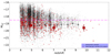 |
Fig. A.1. MUV and redshift distribution of our spectroscopic sample (small red squares). We compared our sample with a photometric one (small black open circles), selected with a magnitude cut of 29.5 in the F277W filter. The big red squares and the big black open circles represents the medians and median absolute deviation of MUV in the same bins of redshift used in this paper (z < 6.5, 6.5 < z < 8.5 and z > 8.5) for our spectroscopic sample and the photometric one, respectively. In both cases, we considered only galaxies brighter than MUV, lim = −18.5 (shown as the dotted pink line). |
To compare the two population distributions, we calculated median values in bins of redshift (z < 6.5, 6.5 < z < 8.5 and z > 8.5 for our spectroscopic sample, as already defined in the paper) and the associated median absolute deviations (big red squares and big black open circles). If we consider only galaxies with MUV < −18.5 (which is the limit discussed in Sect. 3.1), we find a good agreement between the two distributions, meaning that our sample is a good representative of the underlying full population.
All Tables
All Figures
|
Fig. 1. Top-left: Spectroscopic β as a function of the absolute magnitude, MUV, for the entire sample (red points) in the redshift range between z = 4 and z = 14. The other three panels show the relation in redshift bins (z < 6.5, 6.5 < z < 8.5, z > 8.5). The best-fit linear relation for all the individual galaxies is shown with a solid orange line, while the best fit to the median points in bins of MUV (blue crosses) is indicated by a blue solid line. The dotted line shows the MUV = −18.5 limit. In the top-left corner of each panel, we highlight the slope of the best-fit relation. |
| In the text | |
|
Fig. 2. Slope of the β vs. MUV relation in three different redshift bins spanning the range covered by our analysis. |
| In the text | |
|
Fig. 3. Redshift evolution of the spectroscopic β from z = 4 to z = 14. The best-fit linear relation of all the individual galaxies (gray points) is shown with a red solid line, while the best-fit to the medium points in the redshift bins (red circles) is displayed with a red dashed line. Average UV slopes from the literature are also shown for comparison. The blue points are the XBGs studied in Sect. 4. |
| In the text | |
|
Fig. 4. Redshift evolution of the function β − βDW. All galaxies reported in the plot have S/N > 5. Furthermore, the 407 green galaxies shown satisfy the condition MUV < −18.6. The orange points represent the median values of the green points in redshift bins. On the right panel, a histogram of the green points is shown, fit by a Gaussian function with μ = 0.042 ± 0.002 and σ = 0.038 ± 0.001. |
| In the text | |
|
Fig. 5. Spectral stacks of the red galaxy population, as defined in the text, between 1150 and 6700 Å rest-frame. The position of several UV and optical lines is indicated with vertical gray dashed lines. The same panel shows the fit for deriving the optical break. On top of the stack the fit of the UV lines, the [O II] λ3727 Å+[Ne III] λ3868 Å+Hδ lines, the [O III] λ5007 Å+Hβ triplet, and the Hα+[S II] λλ6717 − 6731 lines, as detailed in the text, are shown. The full spectrum is indicated with a blue solid line. The black spectrum is the fitted region, and the red curve represents the best-fit profile. In each panel, fluxes, 1σ uncertainties, and underlying continuum are also indicated for each of the fitted lines highlighted with thin vertical dashed lines. |
| In the text | |
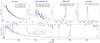 |
Fig. 6. Spectral stacks from Fig. 5 adapted for the XBG subset. |
| In the text | |
|
Fig. 7. Left: Histogram distribution of the escape fractions (estimated indirectly, as explained in the text, and in logarithmic scale) for the subsets of XBGs (blue bars) and red galaxies (red bars), matched in redshift and MUV to the XBGs. Right: Cumulative distribution functions of log10fesc for XBGs and red galaxies (blue dashed and red solid line, respectively). |
| In the text | |
|
Fig. A.1. MUV and redshift distribution of our spectroscopic sample (small red squares). We compared our sample with a photometric one (small black open circles), selected with a magnitude cut of 29.5 in the F277W filter. The big red squares and the big black open circles represents the medians and median absolute deviation of MUV in the same bins of redshift used in this paper (z < 6.5, 6.5 < z < 8.5 and z > 8.5) for our spectroscopic sample and the photometric one, respectively. In both cases, we considered only galaxies brighter than MUV, lim = −18.5 (shown as the dotted pink line). |
| In the text | |
Current usage metrics show cumulative count of Article Views (full-text article views including HTML views, PDF and ePub downloads, according to the available data) and Abstracts Views on Vision4Press platform.
Data correspond to usage on the plateform after 2015. The current usage metrics is available 48-96 hours after online publication and is updated daily on week days.
Initial download of the metrics may take a while.