| Issue |
A&A
Volume 698, June 2025
|
|
|---|---|---|
| Article Number | A75 | |
| Number of page(s) | 13 | |
| Section | Interstellar and circumstellar matter | |
| DOI | https://doi.org/10.1051/0004-6361/202453079 | |
| Published online | 03 June 2025 | |
Modelling carbon chain and complex organic molecules in the DR21(OH) clump
1
Department of Physics and Astronomy, University of Calgary,
Calgary,
Canada
2
Institut de Recherche en Astrophysique et Planétologie, Université de Toulouse, CNRS, UPS, CNES,
Toulouse,
France
3
Department of Astronomy and Astrophysics, Tata Institute of Fundamental Research,
Mumbai
400005,
India
★ Corresponding author: This email address is being protected from spambots. You need JavaScript enabled to view it.
Received:
19
November
2024
Accepted:
14
April
2025
Abstract
Context. Star-forming regions host a large and evolving suite of molecular species. Molecular transition lines, particularly of complex molecules, can reveal the physical and dynamical environment of star formation.
Aims. We aim to study the large-scale structure and environment of high-mass star formation through single-dish observations of CH3CCH, CH3OH, and H2CO.
Methods. We conducted a wide-band spectral survey with the Institut de radioastronomie millimétrique 30 m telescope and the 100 m Green Bank Telescope towards the high-mass star-forming region DR21(OH)/N44. We used a multi-component local thermodynamic equilibrium (LTE) model to determine the large-scale physical environment near DR21(OH) and the surrounding dense clumps. We followed up with a radiative transfer code for CH3OH to look at non-LTE behaviour. We then used a gas-grain chemical model to understand the formation routes of these molecules in their observed environments.
Results. We disentangled multiple components of DR21(OH) in each of the three molecules. We find both a warm and cold component towards both the dusty condensations MM1 and MM2, and a fifth broad, outflow component. We also find warm and cold components towards other dense clumps in our maps: N40, N36, N41, N38, and N48. We find that thermal mechanisms are adequate to produce the observed abundances of H2CO and CH3CCH while non-thermal mechanisms are needed to produce CH3OH. We determine that the production routes of these species are dominated by grain chemistry.
Conclusions. Through a combination of wide-band mapping observations, LTE and non-LTE model analysis, and chemical modelling, the chemical and physical environments of star-forming regions are revealed. This method allows us to disentangle the different velocity and temperature components within our clump-scale beam, a scale that encompasses both the star-forming core and its parent cloud.
Key words: astrochemistry / stars: formation / stars: protostars / ISM: molecules / submillimeter: ISM
© The Authors 2025
 Open Access article, published by EDP Sciences, under the terms of the Creative Commons Attribution License (https://creativecommons.org/licenses/by/4.0), which permits unrestricted use, distribution, and reproduction in any medium, provided the original work is properly cited.
This article is published in open access under the Subscribe to Open model. This email address is being protected from spambots. You need JavaScript enabled to view it. to support open access publication.
1 Introduction
The dynamic evolution of star formation leads to the production of a diverse suite of molecules. Molecular emission thus reveals details about the physical and chemical conditions from which these species arise. In particular, wide-band millimetre and sub-millimetre observations are capable of capturing numerous rotational transition lines which are powerful diagnostics of their environment due to the different excitation conditions each line is sensitive to.
In early-stage protostellar sources in particular, when the accreting protostar is still enshrouded in an envelope, two categories of molecules are distinguished for their diagnostic capabilities: complex organic molecules (COMs; carbon-bearing saturated molecules with ≥6 atoms) and carbon-chain molecules (CCMs; unsaturated hydrocarbons). These species are sensitive to their environment and are valuable tracers alongside more common, simple species such as CO, HCN, or HCO+.
Interstellar COMs are abundant in the hot (T > 100 K) and dense (nH2 > 106 cm−3) cores of star-forming regions (Blake et al. 1987; Caselli et al. 1993; Cazaux et al. 2003; Ceccarelli 2004; see Herbst & van Dishoeck 2009 for a review of these molecules).
On the other hand, CCMs are known to exist in cold (T ≤ 10 K) molecular clouds and starless cores (Avery et al. 1976; Broten et al. 1978; Kroto et al. 1978; Little et al. 1978; Sakai et al. 2010). They are now also known to form in the warm gas enveloping protostellar systems in a process dubbed warm carbon chain chemistry (WCCC; Sakai et al. 2008; Aikawa et al. 2008; Sakai & Yamamoto 2013).
Due to this chemical differentiation, COMs and CCMs can be used to classify protostellar systems. While these species have been used to study star-forming regions, especially hot cores, high-mass star-forming regions (HMSFRs), which are capable of producing stars with M > 8 M⊙, are more difficult to study due to their relative rarity, clustered environments, and quick evolutionary timelines. As the evolutionary processes of HMSFRs are not fully understood, observing their molecular emission is a valuable tool for studying these regions. The first HMSFR found with evidence of WCCC was DR21(OH) (Mookerjea et al. 2012), a nearby and prominent region within Cygnus X.
DR21 (OH) lies 2′ north of the DR21 H II region at a distance of 1.5 kpc (Rygl et al. 2012). Its peak, known as DR21(OH)M or N44, has a total mass of about 103 M⊙ and a density nH2 of 106 cm−3; it has been resolved into two sources, MM1 and MM2 (Woody et al. 1989; Mangum et al. 1991; Motte et al. 2007). MM1 has the stronger continuum emission at millimetre wavelengths (Liechti & Walmsley 1997). Both MM1 and MM2 are thought to be very young, with no visible H II region, and only very weak continuum emission at centimetre wavelengths (Argon et al. 2000). They are thought to be in a pre-ultracompact H II region phase. Dust continuum observations suggest that MM1 is the brighter source (L = 1.7 × 10⁴ L⊙; consistent with a B0V star) and shows evidence of star formation, whereas MM2 (L = 1.2 × 10³ L⊙; early B star), though more massive, is fainter and most likely at an even earlier stage of evolution. These sources have been further differentiated: Zapata et al. (2012) found nine millimetre sources between MM1 (SMA 5–9) and MM2 (SMA 1–4), each with masses in the range 8–24 M⊙; Minh et al. (2012) identified two hot sub-cores in millimetre observations of MM1 corresponding to SMA 6 and 7. The presence of methanol masers (Class I, pumped collisionally) along a bipolar outflow is further evidence that DR21(OH)M is a region of active star formation (Plambeck & Menten 1990; Kogan & Slysh 1998; Kurtz et al. 2004; Araya et al. 2009).
Near DR21(OH)M are several other dense clumps: DR21(OH)S (or N48), DR21(OH)W (N38), DR21(OH)N1 (N41), DR21(OH)N2 (N40), and N36 (Mangum et al. 1991; Chandler et al. 1993; Motte et al. 2007). These sources exist along the DR21 ridge, which consists of filamentary structures that influence collapse (Schneider et al. 2010; Hennemann et al. 2012). N48, N38, and N40 are massive IR-quiet cores noted as possible precursors to high-mass protostars; the lack of IR emission suggests that they are not yet forming a star, but their SiO emission is indicative that an outflow is being powered by a protostellar object (Motte et al. 2007). Mangum et al. (1991) found N48 and N38 to be high-luminosity objects, consistent with B-type stars, but they did not detect any maser emission, which suggests that these sources are in the early stages of star formation. In total, these sources make up a parsec-scale region with a mass of 4900 M⊙ (based on 1.2 mm continuum emission; Schneider et al. 2010).
Interferometric observations have catalogued DR21(OH)M as a rich molecular source that comprises hydrocarbons and COMs (Zapata et al. 2012; Minh et al. 2012; Girart et al. 2013; Orozco-Aguilera et al. 2018). Observations of the larger-scale environment detail the continuum emission and that of simple species such as CO, CS, SiO, N2H+, and HCO+(Richardson et al. 1994; Lai et al. 2003; Motte et al. 2007; Schneider et al. 2010). We aim to link the molecular environment of DR21(OH)M at core scales to the larger clump and filament it resides in. We used single-dish observations to map CH3CCH as a CCM tracer as well as CH3OH and H2CO as COM tracers, and used a local thermodynamic equilibrium (LTE) model to determine the physical parameters of different gaseous components within the DR21 (OH) region. The rest of the paper is structured as follows: Sect. 2 presents the observations and the dataset used, and Sect. 3 the LTE modelling results and analysis. In Sect. 4 we present a chemical evolution model and discuss the findings, and in Sect. 5 provide a brief summary.
2 Observational data
2.1 Observations
We observed DR21 (OH) in multiple frequency ranges with the Institut de radioastronomie millimétrique (IRAM) 30 m telescope and the 100 m Green Bank Telescope (GBT). A detailed summary of these observations is found in Freeman et al. (2023).
The IRAM 30-m observations were completed November 2020 and April 2021 (project codes 021-20 and 122-20, PIs S. Bottinelli and R. Plume). We mapped a 1′ × 1.5′ region in DR 21(OH) in the on-the-fly observational mode with position switching. We observed the frequency ranges 131.2−138.98 GHz and 287.22−295 GHz simultaneously with the Eight MIxer Receiver (EMIR). The offset position was −120′′ horizontally and −240′′ vertically. The map centre is αJ(2000)=20h39m01.00 and δJ(2000)= +42∘22′48′′.0. Data reduction, and the production of maps, was completed with GILDAS/CLASS1. At 291 GHz, the spectral channel width is 781 kHz or 0.80 km s−1, the beam size is 9.3′′, the pixel size is 4.4′′, and the average noise level is 79.7 mK. At 135 GHz, the spectral channel width is 391 kHz or 0.88 km s−1, the beam size is 20.5′′, and the pixel size is 9.7′′. Given the larger beam size, the 135 GHz data will not be discussed in this paper.
The GBT observations were completed in March 2021, in the frequency ranges 84.5−85.75 GHz and 95.55−96.8 GHz using all 16 beams of the Argus focal plane array and the VErsatile GBT Astronomical Spectrometer (VEGAS) spectral line backend (project code 21A-039, PI P. Freeman). We obtained 1′ DAISY on-the-fly maps for both frequency ranges, centred as above, using position-switching for the reference measurements. The spectral sampling with spectrometer mode 2 is 92 kHz in both frequency ranges, or 0.32 km s−1 at 85 GHz and 0.28 km s−1 at 96 GHz. The beam size is 9.2′′ at 96 GHz and 10.0′′ at 85 GHz, both with a pixel size of 2.0′′. The average noise level is 24.0 mK at 85 GHz and 17.7 mK at 96 GHz. The data were reduced and calibrated using GBTIDL2. In Sect. 3, the data are presented in units of TMB. We converted from  using the telescope Beff/Feff values provided by the respective observatories: GBT at 85 GHz, 0.4545; GBT at 96 GHz, 0.3838; IRAM EMIR at 290 GHz, 0.547.
2.2 Species of study
In these datasets we detect numerous lines of CH3CCH, a CCM tracer, and of CH3OH and H2CO, to be used as COM tracers. The lines were identified in CASSIS3 (Vastel et al. 2015) using the Cologne Database for Molecular Spectroscopy4 (CDMS) catalogue (Müller et al. 2005).
Propyne, or methyl acetylene (CH3CCH), is a symmetric rotor with many transitions closely spaced in frequency. Numerous lines are thus captured in a small bandwidth, and are useful for analysis of the physical conditions, especially temperature, in LTE (Irvine et al. 1981; Askne et al. 1984; Kuiper et al. 1984; Bergin et al. 1994). It has long been detected in low- and highmass star-forming regions and is used as a tracer of chemical complexity (Snyder & Buhl 1973; Lovas et al. 1976; Cazaux et al. 2003; Taniguchi et al. 2018; Giannetti et al. 2017; Santos et al. 2022).
Methanol, CH3OH, is the simplest alcohol molecule and an asymmetric top molecule (Ball et al. 1970). It has numerous transitions in the millimetre and sub-millimetre ranges, which are abundant and commonly used as probes of the physical environment. H2CO was the first polyatomic organic molecule detected in space (Snyder et al. 1969), and while not technically a complex species it is chemically associated with larger organic molecules. Both H2CO and CH3OH are formed by the successive hydrogenation of CO on dust grain surfaces, and are precursor molecules to larger COMs (Charnley et al. 1997; Garrod & Widicus Weaver 2013). These two species are detected across interstellar space: in cold clouds, hot cores, outflows, shocks, the Galactic centre, and external galaxies (see Herbst & van Dishoeck 2009, and references therein).
Table 1 lists the transition lines seen in our frequency ranges, with certain conditions based on the sensitivity of our observations. We limited the scope of lines: for CH3CCH an Aij > 1 × 10⁻⁶ s−1 and Eup < 200 K (to account for the a-CH3CCH line that has Eup < 150 K, but has a higher tabulated value when the a- and e-types are combined in CDMS); for H2CO an Aij > 1 × 10⁻⁶ s−1 and Eup < 150 K; for CH3OH an Aij > 2 × 10⁻⁶ s−1 (to remove the 84.5 GHz maser line) and Eup < 150 K. Integrated intensity maps of select lines covering a range of upper energy levels are displayed in Fig. 1.
Class I masers are often found in young star-forming regions, including in DR21(OH) (Ladeyschikov et al. 2019; Slysh et al. 1997; Araya et al. 2009). In particular, the CH3OH line at 84.5 GHz is a known maser in DR21(OH) (Batrla & Menten 1988). These masers, which are collisionally pumped, are unlikely to be well reproduced by LTE. Thus, to be cautious, we did not include this line in our LTE analysis.
Rotational transition lines of selected molecules in the observed frequency ranges, from Freeman et al. (2023).
3 LTE modelling: Results and analysis
An LTE model was used to determine the physical parameters of the observed region – size, line width, column density, excitation temperature, and source velocity. In LTE, we assume the excitation temperature represents the gas temperature. We used a Python-based LTE model based on the CASSIS formalism5 (previously described in Freeman et al. 2023 for a similar analysis of AFGL 2591 and IRAS 20126+4104). The LTE model identifies all molecular transitions for one or more species and simultaneously fits these lines defined by the physical parameters. The resulting fit is the combination of parameters that best reproduces the spectral line profile as determined by a least-squares minimisation (represented as a reduced χ2 value). In the model, we used the CDMS tags6 for each species (Müller et al. 2005). The species types – a- and e-CH3CCH, A- and E-CH3OH, and o- and p-H2CO – were not differentiated, as we did not detect enough lines of each.
In the simplest case, an observed spectral line will arise from one physical gas component modelled by a single Gaussian profile with a systemic velocity (vLSR), line width (Δ vFWHM), and brightness (TA*). However, in the case where the telescope’s beam encompasses multiple physical components, the observed spectra may have to be modelled using multiple Gaussian profiles.
We treated each species, CH3CCH, CH3OH, and H2CO, separately in our analysis. To determine the components of each species, we started with a one-component fit and looped the model over all pixels in the map. When a one-component fit was not adequate, as determined via either a visual inspection of the spectral line profile or the resulting χ2 analysis, we added components as needed. This divided the map into regions described by their own, distinct, physical components. The regions, marked in Fig. 2, correspond to the clumps found in Motte et al. (2007). We gained an idea of what components were necessary based on (a) taking an example spectrum and fitting multiple Gaussians in CASSIS to find velocity and line width information, and (b) knowledge from the literature on what velocity and temperature components we expect to see at this scale. The results for these fits are presented in Table 2. To measure the quality of the fits, we present the reduced χ2 values in Fig. A.1. This reduced value is the χ2 divided by the number of degrees of freedom – the number of data points minus the number of variables – and should be close to 1 for a good fit.
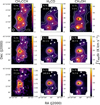 |
Fig. 1 Integrated intensity maps for select transition lines of CH3CCH, H2CO, and CH3OH. The dense clumps as identified in Motte et al. (2007) are shown as stars, with the main clump N44 in black (see also Fig. 2). The quantum states and upper energy level of the transition are listed in the top left of each plot. |
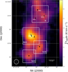 |
Fig. 2 Regions isolated for LTE modelling near and in DR 21(OH), marked in white boxes over an integrated intensity map of the 12 K CH3CCH 50−40 line. From the top, the regions include: N40, N36, and N41 (labelled N); N44; N38; and N48. The dense clumps, as designated by Motte et al. (2007), are marked by stars. |
3.1 N44
All three species required multiple components near DR21 (OH)M, as broad and multi-peaked spectra are seen (Fig. A.2 shows the spectra of the central pixel, marked by the black star in Fig. 1).
We started with two components, N44 1 and N44 2, based on the vlsr values of the dusty condensations MM1 (about −4.1 km s−1) and MM2 (−0.7 km s−1) provided by Mangum et al. (1992), Mookerjea et al. (2012), and Minh et al. (2012). In all three species, we find components with similar characteristics. Table 2 lists the component parameters and Fig. 3 shows the column density maps (Fig. A.9 shows the error).
We find two cooler and extended components in CH3OH 3 and 4 and CH3CCH 1 and 2. We limit the region in Fig. 3 to 18′′, to encompass the MM1 and MM2 regions where the lines are strong enough to fit well. CH3OH 3 (22 K) and CH3CCH 1 (42 K) peak just south-east of MM1 and extend to most of the modelled N44 region. CH3OH 4 (15 K) and CH3CCH 2 (38 K) peak in between MM1 and MM2 and are slightly less extended. They all have the same Δ v = 2.8 km s−1. In the interferometric observations of Minh et al. (2012) and single-dish observations of Weaver et al. (2017) there are CH3OH components of 1820 K. Weaver et al. (2017) also find one component of CH3CCH at 37 K. At these temperatures, our cooler components likely trace the extended envelope around the MM1 and MM2 dusty condensations.
We find two warmer and more concentrated components in CH3OH 1 and 2 and H2CO 1 and 2. CH3OH 1 (82 K) and H2CO 1 (81 K) peak on MM1. CH3OH 2 (75 K) and H2CO 2 (84 K) are the most compact and are concentrated just north of MM2, showing only a few pixels of prominence. These components are broader than the cool components, with a Δ v = 4.0 km s−1. Comparably, in H2CO, Zhao et al. (2024) find a kinetic temperature of 103 K for N44. Their spectral line profile clearly shows two velocity components (visually, similar to ours) but in their model they could not distinguish different components. In CH3OH, Minh et al. (2012) find a 200 K core component and Weaver et al. (2017) find a 93 K component. This suggests that at our spatial scales, on clump scales, we are likely smoothing out the hot gas near the SMA cores, thus the lower temperatures.
For the velocities of each of these components, we find a distinction between those peaking near MM1 or near MM2. Near MM1 the warm component is near −3.6 km s−1 in CH3OH and −4.1 km s−1 in H2CO, while the cold component is around −4.1 to −4.2 km s−1. Near MM2, the warm component is at −0.5 km s−1 while the cold component is at −0.9 km s−1. While our vlsr values (Table 2) do not exactly match previous results, which contain components varying from −5 km s−1 to 1 km s−1 (Mangum et al. 1992; Minh et al. 2012; Girart et al. 2013; Mookerjea et al. 2012), the spatial scales over which we are modelling may provide slightly different average velocities.
A broad feature that is blueshifted relative to the source vlsr of −4.1 km s−1 is seen in both CH3OH 5 and H2CO 3 (Fig. A.3 shows the spectra of a pixel about 6′′ west of MM1 and MM2, where the outflow is most prominent). We fixed this component to a Δ v of 15 km s−1 and a vlsr of −8 km s−1. We are not able to reconcile the temperature of these two species in this component. H2CO is fit well at 80 K, while CH3OH is at 25 K. This could be due to the energy levels of the lines we detect, as CH3OH contains much lower energy lines, or, it could be due to nonthermal behaviour.
We first introduced this broad component based on other, similar features seen the H2CO and CH3OH maps of Zapata et al. (2012) Fig. 2. Their broad lines emanate from SMA 6 and 7 with the blue- to redshifted features going along an E-W gradient. There is a known maser outflow seen in Vallée & Fiege (2006) or Araya et al. (2009), with a redshifted wing of a low-velocity outflow towards the NW. This also corresponds well to the maser observations of Plambeck & Menten (1990) and Kogan & Slysh (1998); the former suggest that the maser emission could be powered by outflows interacting with dense clumps of gas. However, our blueshifted westward component may not correspond to this particular outflow. Instead, it may correspond to the outflow emission in CO(2−1) and SiO presented in Zapata et al. (2012) that differs from their methanol outflow. These are two classic outflow tracers. The CO(2−1) emission features a high-velocity bipolar flow with its blueshifted wing towards the west, and SiO shows a low-velocity flow with the same spatial pattern. This blueshifted feature is also seen in CO and SiO in Lai et al. (2003), Motte et al. (2007), and Schneider et al. (2010). The broad H2CO and CH3OH component we observe, then, is likely tracing the CO outflow and is not associated with the maser outflow.
In the model spectrum (Figs. A.2 and A.3), certain transition lines are underfit in CH3OH. There is known non-thermal emission in this region, identified mainly through the prominent maser emission (Plambeck & Menten 1990; Kogan & Slysh 1998; Kurtz et al. 2004; Araya et al. 2009). Weaver et al. (2017) found two transition lines at 230 and 250 GHz, which are not known as masers, with non-LTE behaviour and suggest they could be powered by similar mechanisms. Our lines at 290 GHz are similarly above the frequency at which any maser lines have been distinguished, but indicate non-LTE behaviour in our models.
To investigate the possible non-LTE behaviour of CH3OH, we used a Markov chain Monte Carlo RADEX (van der Tak et al. 2007) code in CASSIS. Unlike the LTE model, RADEX is too computationally intensive to run over all pixels in the map. We chose to model the central pixel of the map as representative of MM1 and MM2 (Fig. A.2) and a pixel 6′′ (three pixels) west of the central pixel in N44 where the outflow component is seen to be the most prominent (Fig. A.3).
We used the same parameters as in the LTE model for the size, line widths, and velocities. Otherwise, the remaining fitted parameters are in Table 3. We used the VASTEL Database7, which uses the A- and E-CH3OH forms, as there are only collisional coefficients for the separated A- and E- forms. These use p-H2 as the collision species. The isotopic ratio was set at 1.
The results show CH3OH is near LTE with most excitation and kinetic temperatures within 1−10 K of each other. In the centre pixel (Fig. A.2) most lines are just as well represented by the LTE model. In the outflow (Fig. A.3), certain lines are much better represented in the RADEX model. There, the GBT triplet at 96.74 GHz (Eup = 20, 7, 13 K), and the IRAM lines at 290.1, 290.3, and 292.7 GHz (Eup = 49, 75, 71, 64 K). The GBT lines, which are dominated by the colder components in LTE, are likely tracing sub-thermally excited gas. These GBT and IRAM lines show visually the most prominent outflow wings, and could have non-thermal excitation due to the shock conditions.
We tried running the LTE model with adjusted temperatures from these RADEX results. In component 2, a higher temperature does not make a clear difference. In components 3 and 4, a higher temperature from the outflow results produces worse results. Similarly, an adjusted temperature in component 5 produces worse results. However, components 3 and 4 peak near the centre pixel, where the LTE and RADEX temperatures align, and component 5 peaks near the outflow pixel, where similarly the LTE and RADEX temperatures align.
For the other clumps, as they show a similar pattern in the CH3OH models, we discuss the RADEX modelling along with the LTE modelling. The LTE modelling provides an estimate of the gas conditions on a clump scale, while the RADEX modelling provides additional information on the parameters for a single, central pixel.
LTE model results. Values are averaged over a three by three pixel area on the peak Ntot of the clump.
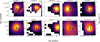 |
Fig. 3 Column density maps, as resulting from an LTE model, for all species (rows) in components (columns) of N44. The cores SMA 7 in MM1 and SMA 3 in MM2 are labelled ‘1’ and ‘2’, respectively, and the clump of N44 is marked by a star (as designated in Zapata et al. 2012 and Motte et al. 2007). CH3OH 5 has been moved to align with H2CO 3, the broad components. Values for all LTE model parameters are listed in Table 2. |
3.2 N48
N48 is a well-studied clump, with Mangum et al. (1991) showing it also as a high luminosity source with a potentially embedded star and Motte et al. (2007) classifying N48 as a massive IR-quiet protostellar source. In our results, a one-component fit worked well for CH3CCH and H2CO for most of the map (Fig. A.4). Figure 4 shows the column density maps for these species, which were found at 34 K and 68 K, respectively (Fig. A.11 shows the error).
In CH3OH, we identify one component at 28 K and another at 8 K (Table 2). They had equal line widths of 3.2 km s−1 and we fixed the velocity of the second component to that of the first component. The region is known to have structure on smaller scales – with the Plateau de Bure Interferometer Bontemps et al. (2010) found five fragments in 1 mm emission and two main fragments in 3 mm emission, while Csengeri et al. (2011a) found two components in H13CN at a vlsr of −2.39 and −4.77 km s−1. Our two components are at −3.83 and −4.03 km s−1, similar, but again likely offset due to the spatial scales and environments we can trace. In addition, Mangum et al. (1991) see an E-W extension in the source. Our second component of CH3OH (Fig. 4) has a westward extension, and towards the edge of the modelled region extends towards the north-west, towards N38.
Similar to N44, there are underfit CH3OH lines in the LTE model. Using RADEX, we fitted two components with very similar Tex, vlsr, and full width at half maximum (FWHM) values. There was a larger Ntot in component 1 and a smaller one for component 2, and, overall, this model better represented both the lower energy GBT lines and the higher energy IRAM lines (Fig. A.4, last column). However, with such similar values we conclude that the gas is in near-LTE.
RADEX model results for CH3OH. The values are for the pixel at the location of the clump noted by Motte et al. (2007).
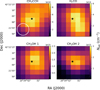 |
Fig. 4 Column density maps for all species in components of the region N48. The clump location is indicated with a star (Motte et al. 2007). |
3.3 N38
N38 is seen as a luminous source with a potentially embedded star and a N–S extension, according to Mangum et al. (1991), with Motte et al. (2007) classifying it as a massive IR-quiet protostellar source. In our data, we identify one component each in CH3CCH and H2CO and two components in CH3OH. Figs. 5, A.10, and A.5 display the column density maps, error maps, and spectra.
Similar to the previous sources, we are seeing warm gas at the scale of the clump. H2CO peaks at 53 K just west of the Motte et al. (2007) clump peak while the CH3CCH component peaks just south of the clump at 29 K. This is similar to other temperature derivations of the region, where Mangum et al. (1992) find two components at 26 and 25 K in NH3 and Zhao et al. (2024) find a H2CO kinetic temperature of 57 K. We are not necessarily smoothing out a hot core here.
In CH3OH, we see one warm, 30 K peak that dominates the fit in the IRAM lines and spatially matching the H2CO peak (Fig. 5). We also find one cold, 8 K, component that dominates the fit in the GBT lines and peaks to the south-east of the warm component. This aligns spatially with the cold CH3OH component that extends from N48 to the north-west (Fig. 4). We infer this cold gas is coming from the extended filament of the DR21 ridge. Similarly, Csengeri et al. (2011b) found this cold extended gas in between N38 and N48 with single-dish observations of N2H+.
Once again, the LTE model under-fits CH3OH lines in both the GBT and IRAM ranges, and we are able to reproduce the lines well in RADEX (Fig. A.5). We find in RADEX one warmer, 25 K, component and one colder, 13 K, component. Overall, the parameters are similar to the LTE model, except with the higher Ntot contained in the warmer component 1 compared to the LTE model where it was in the cold component 2.
3.4 N: N40, N41, and N36
Towards the north region (N), we grouped together N40 (Fig. A.6), N41 (Fig. A.7), and N36 (Fig. A.8), as seen in Fig. 2. The column density maps in Fig. 6 (Fig. A.12 show the error), show that the H2CO is fit well by one component, while CH3CCH requires two components: one 30 K component with a line width of 2.6 km s−1 in between the three clumps identified by Motte et al. (2007), and a 25 K component with a line width of 1.2 km s−1 towards the outer regions of N41 and N36. In CH3OH we identify three components: one warm, 30 K component and two cold, 6 K components, one moderately broad at 3.7 km s−1 and one narrow at 1.2 km s−1 (see also Table 2). The velocities were fixed to that of the first component.
Motte et al. (2007) classify N40 as a massive IR-quiet protostellar source from 1.2 mm continuum emission, yet Bontemps et al. (2010) note it is weak at 3 mm and may be extended, unlike the other dense clumps they study. Compared to our other clumps, we also see weaker emission in this region (Fig. 1). In N48 and N38 the strength of the CH3OH lines with Eup = 49 K, < 21 K are comparable (Figs. A.4 and A.5), while in N40 and N41 the 49 K CH3OH lines are much weaker and the emission is dominated by the cold components.
We fitted each clump separately in RADEX (Figs. A.6, A.7, and A.8). All three clumps were fitted with two warmer components, at ∼30 K and ∼24 K, and one colder component at ∼10 K. As the components are not equally prominent in each clump, we expect to see variation in the RADEX parameters between clumps. In the LTE model, we are capturing the larger-scale trends as we try to find parameters suitable to the whole modelled region. Overall, the RADEX results only varied slightly from the LTE model.
4 Chemical modelling: Results and analysis
The components distinguished by our LTE model show the large-scale environment around many, known core-scale features. DR21(OH), within the larger DR21 ridge, is a young complex with embedded protostars that have not yet disrupted the parent cloud.
In order to determine the possible origin of these molecules in the observed environments, we modelled the species abundances using the NAUTILUS gas-grain code (Ruaud et al. 2016). We did this for all species in all components of DR21(OH), or N44 (we do not use the N44 designation for each component in this section, as all are N44). NAUTILUS uses three phases for chemical evolution – gas, grain surface, and grain mantle and stimulates the abundances over time as a function of different physical conditions – gas density, dust and gas temperature, visual extinction, ultraviolet flux and cosmic ray ionisation. In the code, coupled differential equations describe a network of over 10 000 reactions: 7627 gas-phase reactions and 3799 grain reactions, which involve adsorption onto surfaces, desorption from surfaces, surface reactions, processing within the mantle, and migration between the mantle and the surface. These reactions connect 510 gas-phase species, 225 grain surface species, and 225 grain mantle species.
First, we derived the observed fractional abundances for all components of CH3CCH, H2CO, and CH3OH. We took the ratio of the observed column density for a given component, which we set at the peak value of the LTE model (Sect. 3.1), and the column density of molecular hydrogen, H2. We found the H2 column density at the same position by re-gridding and smoothing the Cao et al. (2022) H2 map in CASA8 onto our grid and beam size. Cao et al. (2022) derived their map using archival data described in Cao et al. (2019): Herschel/PACS 160 μm and James Clerk Maxwell Telescope (JCMT)/SCUBA-2 450 and 850 μm images.
Reports of the H2 to AV conversion value range from  (Rachford et al. 2009; Zhu et al. 2017) to
  (Bohlin et al. 1978; Whittet 1981). In this study, we assumed an ‘average’ value of
  . We used a standard cosmic ray ionisation rate of 1.3 × 10⁻¹⁷ s−1. For the UV field, the NAUTILUS code provided a function of the form S × 108 photons cm−2 s−1 (Ruaud et al. 2016) where S is a scaling factor. We used a scaling factor of 1 to model a general interstellar radiation field. We note that this could be higher in the DR21 environment; however, given the high H2 column densities and resulting values of AV, higher UV field strengths are unlikely to have any effect on the chemistry due to shielding.
We used volume densities, np−H2, similar to the CH3OH RADEX models. We matched the other species components as: CH3OH components 1 and 2 at 1 × 10⁸ to H2CO components 1 and 2; CH3OH component 5 at 5 × 10⁶ to H2CO component 3; CH3OH components 3 and 4 at 2 × 10⁷ to CH3CCH components 1 and 2. This comparison is based on the temperature, line width, and velocity parameters found for each species (Table 2). Such high densities are not unusual for a dense core (Mookerjea et al. 2012; Girart et al. 2013) and are representative of (near) LTE conditions.
Initial ISM abundances in the NAUTILUS model, from Ruaud et al. (2016).
4.1 Model A: Two-stage warmup
In NAUTILUS, we started with a two-stage model (Model A): a cold quiescent cloud followed by a warmup stage powered by embedded protostars. The cold cloud had initial abundances representing the diffuse interstellar medium (ISM; Table 4), a temperature of 10 K, a density of 104 cm−3, a visual extinction of 50 magnitudes, and it evolved for 105 years (Ruaud et al. 2016, as in). Then, in the warmup phase the gas and dust temperature is set to the observed temperature of each pixel found from the LTE model, and the visual extinction is calculated from the average H2 column density (Table 5). These are constant through the warmup stage. There is a discontinuity from the cold cloud stage that is attributed to a rapid change as a result of the formation of the protostar. This stage evolved for another 106 years.
For all three components of H2CO, the warmup stage was adequate to reproduce our observed gas-phase abundances (Fig. 7, top). For components 1 and 2, it takes just over 100 years to produce the observed abundances, while for component 3, the assumed outflow, it takes over 103 years for the abundances to match. The same chemistry applies to all components, on different timescales – at the time the abundances match, the dominant production mechanism changes (Figs. B.1 and B.2). The main production mechanisms at the start are the gas-phase reactions
 (1)
(1)
and
 (2)
(2)
Then, these are replaced by desorption of H2CO off the grain surfaces. For all components, the destruction mechanism follows a similar timeline. H2CO is, at first, solely destroyed by the gasphase reaction
 (3)
(3)
and after 100 or 103 years, depending on the component, the dominant destruction mechanism becomes adsorption onto the grain surface. At this point, the abundance of gas-phase C has sharply decreased.
Overall, the temperatures of ∼80 K are enough to produce the observed abundances. The experimentally determined binding energy of H2CO is reported as 3260 K, which corresponds to a desorption temperature of 110 K (as derived in Penteado et al. 2017). At smaller scales, Zhao et al. (2024) report the H2CO kinetic temperature to be 103 K, so we are likely seeing the hot core smoothed out, and diluting the temperature with the cooler, extended gas. The precursor species of H2CO on grain surfaces is HCO, which has a lower surface binding energy of 1355 K (Penteado et al. 2017), but is highly reactive and therefore not a barrier to forming H2CO (Stantcheva et al. 2002).
As CH3CCH is seen as an envelope molecule, we tried simulating a cloud-edge environment with an AV of 1 (Fig. 7, bottom). In this scenario, the chemical evolution is influenced by the external interstellar radiation field (e.g. Spezzano et al. 2016; Kalvāns 2021). The abundances for both components are reached a few hundred years after the cold cloud stage. At 104 years, there is a sharp decrease in abundance.
The main production route (Fig. B.3), from about 20 years on, is grain surface hydrogenation:
 (4)
(4)
Prior to this, it is the grain surface reaction:
 (5)
(5)
The grain surface production is largely dominant over gas-phase production (as in Hickson et al. 2016; Andron et al. 2018; Calcutt et al. 2019). CH3CCH has a binding energy of 4290 K, requiring a temperature of 144 K for thermal desorption (Penteado et al. 2017). The precursor species, CH2CCH and C2 H3, have binding energies of 3840 and 1760 K, respectively (Penteado et al. 2017), which are both lower than for CH3CCH. Whether or not these species desorb prior to forming CH3CCH, the production of gas-phase CH3CCH is dominated by chemical desorption processes. This is not consistent with CH3CCH being formed in a WCCC scenario. Once the abundance peaks, the main destruction route is photodissociation to H and CH2CCH – assumed to be influenced by the low AV environment.
At about 104 years, there is a sharp change in the CH3CCH formation routes. We determine that, in the low-extinction environment where there is a large H abundance, H atoms are cycling on and off the grain surface. At this abrupt peak, this stops and H is primarily frozen off onto the grains. On the grain surface, H is used up in hydrogenation reactions. Notably, the main reactions during this period are
 (6)
(6)
where CH3CCH stays on the grain surface, and:
 (7)
(7)
Once the grain surface CH2CCH and CCH populations are diminished, the gas-grain cycling of atomic H returns. This also explains the sharp decrease in gas-phase CH3CCH at about 104 years in Fig. 7, as the above reaction does not liberate CH3CCH off the grain surface.
However, DR21(OH) is located within a clustered region, and we do not know if the extent of CH3CCH is truly on the envelope edge. Values of AV up to ∼5 still worked in Model A if the UV field in DR21 is larger than unity. However, modelling CH3CCH with a higher AV corresponding to cloud core conditions (as in H2CO, AV = 50) failed to reproduce the observed abundances at any value of the UV field. In this case, a shock – a sharp spike in temperature and density – was needed to reproduce the CH3CCH abundances. This three-stage shock model, Model B, was also introduced for CH3OH, and is described next.
Parameters for the stages of each NAUTILUS model.
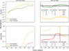 |
Fig. 7 Model A, the two-stage warmup model, for H2CO (top) and CH3CCH (bottom). The 10 K cold cloud stage (left) is followed by a warmup stage where the LTE components are separated based on the temperatures and densities observed. The time axis represents the age of each component independently. The components of each model are in dotted, dashed, or solid lines; red or green lines are the model abundances in the gas phase, yellow the model abundances in the grain phase, and black the observed abundances calculated from the averages in Table 2. |
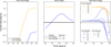 |
Fig. 8 Model B, the three-stage shock model, for CH3OH, simulating a shock. The 10 K cold cloud stage (left) is followed by a sharp increase in density and temperature to simulate a shock (middle) and then a post-shock stage (right), when the gas settles to the LTE conditions observed. The time axis represents the age of each component independently. The LTE components are separated based on their temperatures and densities. The components of each model are in dotted, dashed, or solid lines; blue lines are the model abundances in the gas phase, yellow the model abundances in the grain phase, and black the observed abundances calculated from the averages in Table 2. As C1 and C2 are warmer, we suggest they are still in the shock stage, whereas the cooler C3, C4, and C5 are in a post-shock state. |
4.2 Model B: Three-stage shock
For CH3OH, Model A, with any value of AV or np−H2, did not reproduce the abundances. We then used the approach as in Freeman et al. (2023) and simulated a shock passing through the cloud. Shocks, which can be produced by outflows such as the ones in our source, can liberate grain species into the gas phase causing a sharp increase in gas-phase abundances (Herbst & van Dishoeck 2009; Palau et al. 2017). While we cannot model a shock directly, we simulated shock-induced, non-thermal desorption by implementing a three-stage shock model, Model B: a cold quiescent cloud, a ‘shock’ with a sharp increase in temperature and density, and a post-shock stage where the gas settles to the observed conditions.
The cold cloud is the same as in Model A. In the shock stage, the gas temperature and density evolve as in Palau et al. (2017) for IRAS 20126 (see their Fig. 5, top). This assumes a C-type shock as in Jiménez-Serra et al. (2008) with a shock velocity of 40 km s−1 and a pre-shock density of 104 cm−3. This lasts for 104 years, during which the temperature sharply increased to 2500 K before decreasing, while the density slowly increased from 104 to 8.2 × 104 cm−3, where it stabilised. We fixed the dust temperature to 80 K. Then, in the post-shock phase, we returned the temperature to those observed from the LTE model (as used in the warmup stage above), set the density at 105 cm−2, and allowed the cloud to evolve for a final 106 years (Table 5). For all five components, this reproduced the abundances (Fig. 8).
In component 2, the warm 100 K region, the main, and for the most part only, production route is desorption from the grain surface (Fig. B.4):
 (8)
(8)
We assumed component 1 follows the same route as it has similar physical parameters (Table 2). Due to their higher temperature compared to the other components, we assumed components 1 and 2 are still in a shock stage, as shown in Fig. 8, where their abundances match the model after less than 10 years. The binding energy for CH3OH is 3820 K, corresponding to a desorption temperature of 128 K (Penteado et al. 2017). Similar to H2CO, the precursor species CH3O has a lower binding energy (2655 K), but is a reactive intermediate product (Stantcheva et al. 2002). In Model B and with the lower temperatures found in the LTE model, we see that some non-thermal desorption mechanism after grain surface production is key to producing the gas-phase abundances.
For both the cold and narrow component 4 and the cold and broad component 5, chemical desorption reactions dominate the production of gas-phase CH3OH through the reactions (Figs. B.5 and B.6)
 (9)
(9)
and
 (10)
(10)
This is dominant over 106 years in component 4. For component 5, after 104 years, gas-phase dissociative recombination becomes important:
 (11)
(11)
We assumed these colder components are in the post-shock stage (see Fig. 8). Their model abundances are slightly overproduced until about 105 years, where they sharply decrease. In the cold components, like component 2 above, we see a non-thermal desorption method is necessary. Unlike component 2, there are a number of different reactions that contribute to the formation of CH3OH. There are sharp peaks in some of these routes, namely for Eq. (10). This reaction varies depending on the availability of grain surface H to react. For all components, the main destruction route is adsorption to the grain surface until about 105 years. After that, in all components, there are contributions from gas-phase ion-molecule reactions.
To see if the timescales are physically realistic, we looked at the outflow. For a flow moving at 7 km s−1 (from component N44 5, Table 2), to span 10′′ (Fig. 3; Zapata et al. 2012, Fig. 2), it would need to be 1.6 × 10⁴ years old. This is less than the time it takes for all five components to match model and observed abundances in the post-shock stage.
We find that in higher-density models the same evolution occurs on a faster timescale. We tried to use the RADEX densities in Model B as we had for Model A to reconcile the results of our different analyses. If the RADEX densities were used in the post-shock stage, the abundances would match at a few 103 years for components 3, 4, and 5. However, there would be a sharp density jump from the shock stage to the post-shock stage in this scenario, for which we have no explanation. We tried using the RADEX densities in the shock stage, and the CH3OH was destroyed quickly. However, in addition to the abundances not matching, we have no basis for such high densities in the shock stage as we used a previously parametrised shock. Different type shocks have been explored for example in L1157 (James et al. 2020), but it is out of the scope of this paper. We can only conclude that CH3OH need some form of non-thermal desorption to produce the observed abundances.
We can speculate on possible sources powering non-thermal desorption in DR21(OH). There are numerous outflows seen emanating from MM1 and MM2, including the previously discussed molecular blueshifted outflow and the E-W CH3OH maser outflows, which contain other species such as H2CO and H13CO+(Zapata et al. 2012; Orozco-Aguilera et al. 2018) as well as thermal CH3OH emission. A N–S H2CS outflow is seen from MM1 with rotation temperatures of 40−60 K, where lines of CH3OH are also detected (Minh et al. 2011, 2012). They suggest CH3OH could arise from the same mechanism as H2CS : non-thermal desorption from outflows interacting with the surrounding gas. While we cannot discern the exact sources of the non-thermal desorption in the CH3OH components, the clustered cores of MM1 and MM2 are evidently producing multiple sites of turbulent gas. Further modelling of higher spatial resolution data is needed to determine the structure of DR21(OH) and connect it to the potential molecular formation routes.
5 Summary
We have presented IRAM and GBT observations mapping DR21(OH) at 10′′ resolution. We used CH3CCH, CH3OH and H2CO emission lines to determine the physical parameters of the different gaseous environments in the region, connecting the core scales to the larger clump and filament scales. Our main findings are:
DR21(OH) main, or N44, is found to have ∼80 K and ∼30 K components near both MM1 and MM2, interpreted as the warmer inner core and the cooler envelope. The gaseous components of MM1 and MM2 are differentiated spatially on our maps and in velocity – MM1 is near −3.6 to −4.2 km s−1, while MM2 is near −0.5 to −0.9 km s−1. H2CO and CH3OH also show a broad, blueshifted outflow component that is not associated with the maser outflows of this region but with a molecular outflow seen previously in CO and SiO;
Chemical modelling indicates that H2CO can be produced in the warmup stage through thermal mechanisms, CH3CCH can be produced in the warmup stage in an environment with low AV, and CH3OH needs a non-thermal desorption mechanism to produce the observed abundances. For CH3CCH and CH3OH especially, grain surface production is important for reproducing their gas-phase abundances;
Other dusty condensations in the region show warm, ∼30 K, gas with similar line widths and velocities as those of N44. The cold components seen are likely non-LTE and represent sub-thermally excited gas.
With a sophisticated LTE model we are able to use large-scale single-dish data to disentangle different temperature and velocity components of star-forming clumps and cores. This is useful even for complicated species such as CH3OH, as we are able to apply the model to the whole map along with targeted use of the more computationally expensive RADEX. The LTE model allows us to confidently determine the abundances of each of these species, which is essential for determining the chemical evolution of the region.
Data availability
The supplemental figures in the Appendix can be found at https://zenodo.org/records/15258578.
Acknowledgements
This work is based on observations carried out under project numbers 021-20 and 122-20 with the 30-m telescope. IRAM is supported by INSU/CNRS (France), MPG (Germany) and IGN (Spain). The Green Bank Observatory is a facility of the National Science Foundation operated under cooperative agreement by Associated Universities, Inc. We would like to thank the anonymous referee for their thoughtful and constructive comments. PF would like to thank L. Morgan and D. Frayer at the GBT/NRAO for their help developing observing scripts as well as GBTIDL scripts for ARGUS calibration and reduction, as well as P. Torne and M. Rodriguez at IRAM for their help observing with the IRAM telescope. PF and RP would like to thank K. Qiu and Y. Cao for providing the H2 column density maps. PF and RP acknowledge the support of the Natural Sciences and Engineering Research Council of Canada (NSERC), through the Canada Graduate Scholarships – Doctoral, Michael Smith Foreign Study Supplement, and Discovery Grant programs. As researchers at the University of Calgary, PF and RP acknowledge and pay tribute to the traditional territories of the peoples of Treaty 7, which include the Blackfoot Confederacy (comprised of the Siksika, the Piikani, and the Kainai First Nations), the Tsuut’ ina First Nation, and the Stoney Nakoda (including Chiniki, Bearspaw, and Goodstoney First Nations). The City of Calgary is also home to the Métis Nation of Alberta Districts 5 and 6.
References
- Aikawa, Y., Wakelam, V., Garrod, R. T., & Herbst, E., 2008, ApJ, 674, 984 [NASA ADS] [CrossRef] [Google Scholar]
- Andron, I., Gratier, P., Majumdar, L., et al. 2018, MNRAS, 481, 5651 [NASA ADS] [CrossRef] [Google Scholar]
- Araya, E. D., Kurtz, S., Hofner, P., & Linz, H., 2009, ApJ, 698, 1321 [Google Scholar]
- Argon, A. L., Reid, M. J., & Menten, K. M., 2000, ApJS, 129, 159 [Google Scholar]
- Askne, J., Hoglund, B., Hjalmarson, A., & Irvine, W. M., 1984, A&A, 130, 311 [NASA ADS] [Google Scholar]
- Avery, L. W., Broten, N. W., MacLeod, J. M., Oka, T., & Kroto, H. W., 1976, ApJ, 205, L173 [NASA ADS] [CrossRef] [Google Scholar]
- Ball, J. A., Gottlieb, C. A., Lilley, A. E., & Radford, H. E., 1970, ApJ, 162, L203 [NASA ADS] [CrossRef] [Google Scholar]
- Batrla, W., & Menten, K. M., 1988, ApJ, 329, L117 [NASA ADS] [CrossRef] [Google Scholar]
- Bergin, E. A., Goldsmith, P. F., Snell, R. L., & Ungerechts, H., 1994, ApJ, 431, 674 [NASA ADS] [CrossRef] [Google Scholar]
- Blake, G. A., Sutton, E. C., Masson, C. R., & Phillips, T. G., 1987, ApJ, 315, 621 [Google Scholar]
- Bohlin, R. C., Savage, B. D., & Drake, J. F., 1978, ApJ, 224, 132 [Google Scholar]
- Bontemps, S., Motte, F., Csengeri, T., & Schneider, N., 2010, A&A, 524, A18 [NASA ADS] [CrossRef] [EDP Sciences] [Google Scholar]
- Broten, N. W., Oka, T., Avery, L. W., MacLeod, J. M., & Kroto, H. W., 1978, ApJ, 223, L105 [NASA ADS] [CrossRef] [Google Scholar]
- Calcutt, H., Willis, E. R., Jørgensen, J. K., et al. 2019, A&A, 631, A137 [NASA ADS] [CrossRef] [EDP Sciences] [Google Scholar]
- Cao, Y., Qiu, K., Zhang, Q., et al. 2019, ApJS, 241, 1 [Google Scholar]
- Cao, Y., Qiu, K., Zhang, Q., & Li, G.-X. 2022, ApJ, 927, 106 [NASA ADS] [CrossRef] [Google Scholar]
- Caselli, P., Hasegawa, T. I., & Herbst, E., 1993, ApJ, 408, 548 [Google Scholar]
- Cazaux, S., Tielens, A. G. G. M., Ceccarelli, C., et al. 2003, ApJ, 593, L51 [CrossRef] [Google Scholar]
- Ceccarelli, C., 2004, in Star Formation in the Interstellar Medium: In Honor of David Hollenbach, eds. D. Johnstone, F. C. Adams, D. N. C. Lin, D. A. Neufeeld, & E. C. Ostriker, Astronomical Society of the Pacific Conference Series, 323, 195 [NASA ADS] [Google Scholar]
- Chandler, C. J., Gear, W. K., & Chini, R., 1993, MNRAS, 260, 337 [NASA ADS] [Google Scholar]
- Charnley, S. B., Tielens, A. G. G. M., & Rodgers, S. D., 1997, ApJ, 482, L203 [NASA ADS] [CrossRef] [Google Scholar]
- Csengeri, T., Bontemps, S., Schneider, N., Motte, F., & Dib, S. 2011a, A&A, 527, A135 [NASA ADS] [CrossRef] [EDP Sciences] [Google Scholar]
- Csengeri, T., Bontemps, S., Schneider, N., et al. 2011b, ApJ 740, L5 [NASA ADS] [CrossRef] [Google Scholar]
- Freeman, P., Bottinelli, S., Plume, R., et al. 2023, A&A, 678, A18 [NASA ADS] [CrossRef] [EDP Sciences] [Google Scholar]
- Garrod, R. T., & Widicus Weaver, S. L., 2013, Chem. Rev., 113, 8939 [Google Scholar]
- Giannetti, A., Leurini, S., Wyrowski, F., et al. 2017, A&A, 603, A33 [NASA ADS] [CrossRef] [EDP Sciences] [Google Scholar]
- Girart, J. M., Frau, P., Zhang, Q., et al. 2013, ApJ, 772, 69 [NASA ADS] [CrossRef] [Google Scholar]
- Hennemann, M., Motte, F., Schneider, N., et al. 2012, A&A, 543, L3 [NASA ADS] [CrossRef] [EDP Sciences] [Google Scholar]
- Herbst, E., & van Dishoeck, E. F., 2009, ARA&A, 47, 427 [NASA ADS] [CrossRef] [Google Scholar]
- Hickson, K. M., Wakelam, V., & Loison, J.-C., 2016, Mol. Astrophys., 3, 1 [CrossRef] [Google Scholar]
- Irvine, W. M., Hoglund, B., Friberg, P., Askne, J., & Ellder, J., 1981, ApJ, 248, L113 [NASA ADS] [CrossRef] [Google Scholar]
- James, T. A., Viti, S., Holdship, J., & Jiménez-Serra, I., 2020, A&A, 634, A17 [EDP Sciences] [Google Scholar]
- Jiménez-Serra, I., Caselli, P., Martín-Pintado, J., & Hartquist, T. W., 2008, A&A, 482, 549 [NASA ADS] [CrossRef] [EDP Sciences] [Google Scholar]
- Kalvāns, J., 2021, ApJ, 910, 54 [CrossRef] [Google Scholar]
- Kogan, L., & Slysh, V., 1998, ApJ, 497, 800 [NASA ADS] [CrossRef] [Google Scholar]
- Kroto, H. W., Kirby, C., Walton, D. R. M., et al. 1978, ApJ, 219, L133 [NASA ADS] [CrossRef] [Google Scholar]
- Kuiper, T. B. H., Kuiper, E. N. R., Dickinson, D. F., Turner, B. E., & Zuckerman, B., 1984, ApJ, 276, 211 [NASA ADS] [CrossRef] [Google Scholar]
- Kurtz, S., Hofner, P., & Álvarez, C. V., 2004, ApJS, 155, 149 [Google Scholar]
- Ladeyschikov, D. A., Bayandina, O. S., & Sobolev, A. M., 2019, AJ, 158, 233 [NASA ADS] [CrossRef] [Google Scholar]
- Lai, S.-P., Girart, J. M., & Crutcher, R. M., 2003, ApJ, 598, 392 [NASA ADS] [CrossRef] [Google Scholar]
- Liechti, S., & Walmsley, C. M., 1997, A&A, 321, 625 [NASA ADS] [Google Scholar]
- Little, L. T., MacDonald, G. H., Riley, P. W., & Matheson, D. N., 1978, MNRAS, 183, 45 [Google Scholar]
- Lovas, F. J., Johnson, D. R., Buhl, D., & Snyder, L. E., 1976, ApJ, 209, 770 [NASA ADS] [CrossRef] [Google Scholar]
- Mangum, J. G., Wootten, A., & Mundy, L. G., 1991, ApJ, 378, 576 [Google Scholar]
- Mangum, J. G., Wootten, A., & Mundy, L. G., 1992, ApJ, 388, 467 [NASA ADS] [CrossRef] [Google Scholar]
- Minh, Y. C., Liu, S. Y., Chen, H. R., & Su, Y. N., 2011, ApJ, 737, L25 [NASA ADS] [CrossRef] [Google Scholar]
- Minh, Y. C., Chen, H.-R., Su, Y.-N., & Liu, S.-Y. 2012, JKAS, 45, 157 [Google Scholar]
- Mookerjea, B., Hassel, G. E., Gerin, M., et al. 2012, A&A, 546, A75 [NASA ADS] [CrossRef] [EDP Sciences] [Google Scholar]
- Motte, F., Bontemps, S., Schilke, P., et al. 2007, A&A, 476, 1243 [NASA ADS] [CrossRef] [EDP Sciences] [Google Scholar]
- Müller, H. S., Schlöder, F., Stutzki, J., & Winnewisser, G., 2005, J. Mol. Struct., 742, 215 [Google Scholar]
- Orozco-Aguilera, M. T., Hernández-Gómez, A., & Zapata, L. A., 2018, AJ, 157, 20 [Google Scholar]
- Palau, A., Walsh, C., Sánchez-Monge, Á., et al. 2017, MNRAS, 467, 2723 [NASA ADS] [Google Scholar]
- Penteado, E. M., Walsh, C., & Cuppen, H. M., 2017, ApJ, 844, 71 [Google Scholar]
- Plambeck, R. L., & Menten, K. M., 1990, ApJ, 364, 555 [Google Scholar]
- Rachford, B. L., Snow, T. P., Destree, J. D., et al. 2009, ApJS, 180, 125 [NASA ADS] [CrossRef] [Google Scholar]
- Richardson, K. J., Sandell, G., Cunningham, C. T., & Davies, S. R., 1994, A&A, 286, 555 [NASA ADS] [Google Scholar]
- Ruaud, M., Wakelam, V., & Hersant, F., 2016, MNRAS, 459, 3756 [Google Scholar]
- Rygl, K. L. J., Brunthaler, A., Sanna, A., et al. 2012, A&A, 539, A79 [NASA ADS] [CrossRef] [EDP Sciences] [Google Scholar]
- Sakai, N., & Yamamoto, S., 2013, Chem. Rev., 113, 8981 [Google Scholar]
- Sakai, N., Sakai, T., Hirota, T., & Yamamoto, S., 2008, ApJ, 672, 371 [Google Scholar]
- Sakai, N., Shiino, T., Hirota, T., Sakai, T., & Yamamoto, S., 2010, ApJ, 718, L49 [NASA ADS] [CrossRef] [Google Scholar]
- Santos, J. C., Bronfman, L., Mendoza, E., et al. 2022, ApJ, 925, 3 [NASA ADS] [CrossRef] [Google Scholar]
- Schneider, N., Csengeri, T., Bontemps, S., et al. 2010, A&A, 520, A49 [CrossRef] [EDP Sciences] [Google Scholar]
- Slysh, V. I., Kalenskii, S. V., Val’tts, I. E., & Golubev, V. V., 1997, ApJ, 478, L37 [NASA ADS] [CrossRef] [Google Scholar]
- Snyder, L. E., & Buhl, D., 1973, Nat. Phys., 243, 45 [Google Scholar]
- Snyder, L. E., Buhl, D., Zuckerman, B., & Palmer, P., 1969, PRL, 22, 679 [Google Scholar]
- Spezzano, S., Bizzocchi, L., Caselli, P., Harju, J., & Brünken, S., 2016, A&A, 592, L11 [NASA ADS] [CrossRef] [EDP Sciences] [Google Scholar]
- Stantcheva, T., Shematovich, V. I., & Herbst, E., 2002, A&A, 391, 1069 [NASA ADS] [CrossRef] [EDP Sciences] [Google Scholar]
- Taniguchi, K., Saito, M., Majumdar, L., et al. 2018, ApJ, 866, 150 [NASA ADS] [CrossRef] [Google Scholar]
- Vallée, J. P., & Fiege, J. D., 2006, ApJ, 636, 332 [CrossRef] [Google Scholar]
- van der Tak, F. F. S., Black, J. H., Schöier, F. L., Jansen, D. J., & van Dishoeck, E. F., 2007, A&A, 468, 627 [NASA ADS] [CrossRef] [EDP Sciences] [Google Scholar]
- Vastel, C., Bottinelli, S., Caux, E., Glorian, J. M., & Boiziot, M., 2015, in SF2A2015: Proceedings of the Annual meeting of the French Society of Astronomy and Astrophysics, 313 [Google Scholar]
- Weaver, S. L. W., Laas, J. C., Zou, L., et al. 2017, ApJS, 232, 3 [NASA ADS] [CrossRef] [Google Scholar]
- Whittet, D. C. B., 1981, MNRAS, 196, 469 [NASA ADS] [CrossRef] [Google Scholar]
- Woody, D. P., Scott, S. L., Scoville, N. Z., et al. 1989, ApJ, 337, L41 [Google Scholar]
- Zapata, L. A., Loinard, L., Su, Y. N., et al. 2012, ApJ, 744, 86 [Google Scholar]
- Zhao, X., Tang, X. D., Henkel, C., et al. 2024, A&A, 687, A207 [NASA ADS] [CrossRef] [EDP Sciences] [Google Scholar]
- Zhu, H., Tian, W., Li, A., & Zhang, M., 2017, MNRAS, 471, 3494 [NASA ADS] [CrossRef] [Google Scholar]
All Tables
Rotational transition lines of selected molecules in the observed frequency ranges, from Freeman et al. (2023).
LTE model results. Values are averaged over a three by three pixel area on the peak Ntot of the clump.
RADEX model results for CH3OH. The values are for the pixel at the location of the clump noted by Motte et al. (2007).
All Figures
|
Fig. 1 Integrated intensity maps for select transition lines of CH3CCH, H2CO, and CH3OH. The dense clumps as identified in Motte et al. (2007) are shown as stars, with the main clump N44 in black (see also Fig. 2). The quantum states and upper energy level of the transition are listed in the top left of each plot. |
| In the text | |
|
Fig. 2 Regions isolated for LTE modelling near and in DR 21(OH), marked in white boxes over an integrated intensity map of the 12 K CH3CCH 50−40 line. From the top, the regions include: N40, N36, and N41 (labelled N); N44; N38; and N48. The dense clumps, as designated by Motte et al. (2007), are marked by stars. |
| In the text | |
|
Fig. 3 Column density maps, as resulting from an LTE model, for all species (rows) in components (columns) of N44. The cores SMA 7 in MM1 and SMA 3 in MM2 are labelled ‘1’ and ‘2’, respectively, and the clump of N44 is marked by a star (as designated in Zapata et al. 2012 and Motte et al. 2007). CH3OH 5 has been moved to align with H2CO 3, the broad components. Values for all LTE model parameters are listed in Table 2. |
| In the text | |
|
Fig. 4 Column density maps for all species in components of the region N48. The clump location is indicated with a star (Motte et al. 2007). |
| In the text | |
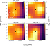 |
Fig. 5 Same as Fig. 4 but for the clump N38. |
| In the text | |
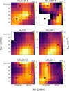 |
Fig. 6 Same as Fig. 4 but for the N region, containing the clumps N40, N41, and N36. |
| In the text | |
|
Fig. 7 Model A, the two-stage warmup model, for H2CO (top) and CH3CCH (bottom). The 10 K cold cloud stage (left) is followed by a warmup stage where the LTE components are separated based on the temperatures and densities observed. The time axis represents the age of each component independently. The components of each model are in dotted, dashed, or solid lines; red or green lines are the model abundances in the gas phase, yellow the model abundances in the grain phase, and black the observed abundances calculated from the averages in Table 2. |
| In the text | |
|
Fig. 8 Model B, the three-stage shock model, for CH3OH, simulating a shock. The 10 K cold cloud stage (left) is followed by a sharp increase in density and temperature to simulate a shock (middle) and then a post-shock stage (right), when the gas settles to the LTE conditions observed. The time axis represents the age of each component independently. The LTE components are separated based on their temperatures and densities. The components of each model are in dotted, dashed, or solid lines; blue lines are the model abundances in the gas phase, yellow the model abundances in the grain phase, and black the observed abundances calculated from the averages in Table 2. As C1 and C2 are warmer, we suggest they are still in the shock stage, whereas the cooler C3, C4, and C5 are in a post-shock state. |
| In the text | |
Current usage metrics show cumulative count of Article Views (full-text article views including HTML views, PDF and ePub downloads, according to the available data) and Abstracts Views on Vision4Press platform.
Data correspond to usage on the plateform after 2015. The current usage metrics is available 48-96 hours after online publication and is updated daily on week days.
Initial download of the metrics may take a while.