| Issue |
A&A
Volume 677, September 2023
|
|
|---|---|---|
| Article Number | A127 | |
| Number of page(s) | 15 | |
| Section | Interstellar and circumstellar matter | |
| DOI | https://doi.org/10.1051/0004-6361/202245213 | |
| Published online | 19 September 2023 | |
Protostellar Interferometric Line Survey of the Cygnus-X region (PILS-Cygnus)
The role of the external environment in setting the chemistry of protostars★
1
Niels Bohr Institute, University of Copenhagen,
Øster Voldgade 5–7,
1350
Copenhagen K., Denmark
e-mail: This email address is being protected from spambots. You need JavaScript enabled to view it.
2
Institute of Astronomy, Faculty of Physics, Astronomy and Informatics, Nicolaus Copernicus University,
Grudziadzka 5,
87–100
Torun, Poland
3
Departments of Astronomy and Chemistry, University of Virginia,
Charlottesville, VA
22904, USA
Received:
14
October
2022
Accepted:
25
June
2023
Abstract
Context. Molecular lines are commonly detected towards protostellar sources. However, to get a better understanding of the chemistry of these sources we need unbiased molecular surveys over a wide frequency range for as many sources as possible to shed light on the origin of this chemistry, particularly any influence from the external environment.
Aims. We present results from the PILS-Cygnus survey of ten intermediate- to high-mass protostellar sources in the nearby Cygnus-X complex, through high angular resolution interferometric observations over a wide frequency range.
Methods. Using the Submillimeter Array (SMA), a spectral line survey of ten sources was performed in the frequency range 329–361 GHz, with an angular resolution of ~1″.5, or ~2000 AU at a source distance of 1.3 kpc from the Sun. Spectral modelling was performed to identify molecular emission and determine column densities and excitation temperatures for each source. Emission maps were made to study the morphology of emission. Finally, emission properties were compared across the sample.
Results. We detect CH3OH towards nine of the ten sources, with CH3OCH3 and CH3OCHO towards three sources. We further detect CH3CN towards four sources. Towards five sources the chemistry is spatially differentiated, meaning that different species peak at different positions and are offset from the peak continuum emission. Low levels of deuteration are detected towards four sources in HDO emission, whereas deuterated complex organic molecule emission is detected towards one source (CH2DOH towards N63). The chemical properties of each source do not correlate with their position in the Cygnus-X complex, nor do the distance or direction to the nearest OB associations. However, the five sources located in the DR21 filament do appear to show less line emission compared to the five sources outside the filament.
Conclusions. This work shows how important wide frequency coverage observations are combined with high angular resolution observations for studying the protostellar environment. Furthermore, based on the ten sources observed here, the external environment appears to only play a minor role in setting the chemical environment on these small scales (<2000 AU).
Key words: astrochemistry / stars: formation / stars: protostars / ISM: molecules / submillimeter: ISM
Appendices are only available in electronic form at Zenedo.org, https://zenodo.org/deposit/8200687
© The Authors 2023
 Open Access article, published by EDP Sciences, under the terms of the Creative Commons Attribution License (https://creativecommons.org/licenses/by/4.0), which permits unrestricted use, distribution, and reproduction in any medium, provided the original work is properly cited.
This article is published in open access under the Subscribe to Open model. This email address is being protected from spambots. You need JavaScript enabled to view it. to support open access publication.
1 Introduction
The molecular emission observed in and near star-forming regions is an important tool with which the physical conditions and evolution of protostars can be inferred. The molecules that cause the emission range from the simplest and most abundant molecules that trace the large-scale structure of the envelopes surrounding the newly formed stars, to the complex organic molecules (COMs; molecules with at least six atoms and one or more carbon atoms; Herbst & van Dishoeck 2009) that are observed closer to the newly formed star, in the warm inner regions of the envelope (‘hot cores’; e.g. Kurtz et al. 2000; Cesaroni et al. 2010; Jørgensen et al. 2016). Different molecules therefore trace different regions in and near newly formed stars (Tychoniec et al. 2021) and observing as many different molecules, both simple and complex, and as many of their transitions as possible is necessary to get a better understanding of the conditions and evolution of protostars.
Simple di- and tri-atomic molecules typically form directly in the gas phase (Herbst & van Dishoeck 2009). The historical picture of the origin of COMs has been that they primarily form on dust grains at cold temperatures, and that they are then released into the gas phase at T ~ 100 K, where they can then be observed directly at sub-millimetre wavelengths in hot cores. However, it has been proposed that COMs can also be sputtered off the icy dust-mantles by shocks from jets and outflows (e.g. Avery & Chiao 1996; Jørgensen et al. 2004a; Arce et al. 2008; Sugimura et al. 2011; Lefloch et al. 2017), shocks from material accreted from the envelope onto the disc (e.g. Podio et al. 2015; Artur de la Villarmois et al. 2018; Csengeri et al. 2018, 2019), from explosive events near forming stars (e.g. Orion KL; Zapata et al. 2011; Orozco-Aguilera et al. 2017), and from UV irradiation of the outflow cavity walls (e.g. Drozdovskaya et al. 2015). Some of these mechanisms have been invoked to interpret why COM emission is sometimes observed to be offset from the main continuum peak, where Τ > 100 K. The dominant process in releasing COMs frozen out on dust grains into the gas phase is therefore often unclear (e.g. Belloche et al. 2020; van der Walt et al. 2021). This understanding is necessary to properly interpret the chemistry, both of COMs and the simpler molecules.
Furthermore, the observed chemistry may not only depend on the local conditions, but the history of the large-scale or external environment may play a role as well. The proximity to bright UV-radiation sources could influence the chemistry as it heats up the environment surrounding the newly formed stars, for example studies of photon-dominated regions (PDRs), near OB stars (Goicoechea et al. 2006; van der Wiel et al. 2009; Taniguchi et al. 2021). Moreover, most stars, particularly higher-mass stars, form in dense hubs where filaments intersect (e.g. Motte et al. 2018), and it is unclear if the close proximity between forming stars in such a dense environment has any effect on the chemistry. Therefore, whether it is the local conditions or the external environment that sets the chemical complexity of newly formed stars is still an open question.
To use the full potential of chemistry and to address these questions, we need to observe emission from as many molecules and their transitions as possible, which requires broad frequency coverage. This has historically been expensive observationally, which resulted in surveys that had to choose narrow frequency bands covering only a select few molecules (e.g. Jørgensen et al. 2007; Öberg et al. 2014; Stephens et al. 2019; Belloche et al. 2020) or full line surveys of a limited number of sources (e.g. Jørgensen et al. 2016; Codella et al. 2017). This situation has changed in recent years with the introduction at the Submillimeter Array (SMA) of the SWARM1 correlator, which is capable of 48 GHz frequency coverage in one sweep at the time of writing (32 GHz at the time data for this work were acquired).
It is important to observe a large number of sources in a single cloud, covering as broad a frequency range as possible. These sources should be observed at high angular resolution so that the spatial origin of molecular emission can be localised and any ambiguities in the physical origin of emission can be removed as best as possible (e.g. Jørgensen et al. 2016): hot core, outflow, envelope, etc. The reason for choosing a single cloud is to, as best as possible, avoid distance uncertainties, while at the same time also ensuring that the sources observed share common initial conditions.
To demonstrate and exemplify what can be done with observations over such a broad frequency range, data of the single source CygX-N30 (N30) were presented in the first-results paper of the Protosteller Interferometric Line Survey of the Cygnus-X region (PILS-Cygnus; van der Walt et al. 2021). The PILS-Cygnus survey is a molecular line and continuum survey of ten sources located in the Cygnus-X star-forming region. It utilised the SWARM correlator on the SMA to take inventory of the chemical variability throughout the Cygnus-X region. The first results from the survey are that the origin of COM emission detected towards this source are from a combination of thermal heating from newly formed stars (the canonical hot core scenario) and accretion of material onto a disc-like structure. The authors further identified chemical differentiation along a linear gradient and between O-bearing species that have peak emission close to one continuum source, while N-and S-bearing species have emission peaks closer to the second source. The authors report low levels of deuteration with only HDO detected towards this source and an upper limit of D/H < 0.1% derived for CH2DOH, which they attribute to warm temperatures of formation, >30 K, with inefficient deuterium fractionation.
Various results utilising parts of the entire sample have already been published. When looking towards the entire sample, two results stand out. First, the properties of the protostellar envelopes (e.g. mass, density and temperature structure) appear to be similar to both low- and high-mass protostars in general, when scaled with luminosity (Pitts et al. 2022). Second, the outflows from these sources also appear similar to low-and high-mass sources, again when scaled with the luminosity (Skretas & Kristensen 2022). These two results suggest that the PILS-Cygnus sources are not special when it comes to envelope structure as well as accretion and ejection processes. However, the question remains whether the chemistry is or has been affected by the clustered environment or the proximity to the nearby bright OB association. This question can only be addressed by analysing line emission from the full data set, which is presented here.
We present here the full data set and analysis of the PILS-Cygnus programme for the first time, where ten sources were observed at a uniform frequency coverage, spatial resolution and sensitivity with the SMA. The focus of this paper is on the spectral line properties of the dataset, and thus the chemical properties of the sources. Apart from addressing the above-mentioned science questions, this paper also serves as the data-release paper for this survey. The paper is organised as follows: Sect. 2 describes the observational setup and data reduction procedure, followed by Sect. 3 in which the results of the data analysis are presented. In Sect. 4, a discussion of the results are given, with a conclusion and summary in Sect. 5.
2 Observations
2.1 Sample selection
The PILS-Cygnus sample consists of ten intermediate- and high-mass sources (see Table 1) located in the nearby Cygnus-X complex (~1.3–1.5 kpc; Table 1). These sources were first selected from the catalogue of Kryukova et al. (2014), who tabulated the bolometric luminosities of ~1800 protostars in the Cygnus-X complex. These luminosities were based on Spitzer IRAC and MIPS observations of the complex, and from there, the bolomet-ric luminosity was inferred based on the methodology outlined in Kryukova et al. (2012). These were then compared to the catalogue of Motte et al. (2007), who observed a large part of the Cygnus-X complex at a wavelength of 1.2 mm with the IRAM-30m telescope. From these two catalogues, we identified the most luminous and massive sources.
The next step in the selection process was to check for signs of current and active star formation. This was done using Herschel-HIFI observations of the H2O 202−111 transition at 988 GHz (San José-García 2015). This particular transition is an excellent outflow and shock tracer (e.g. van Dishoeck et al. 2021), associated with embedded star formation. Most of these sources were also observed in SiO 2−1 emission (Motte et al. 2007), and were found to be bright in this transition. This corroborates that these sources are embedded sources driving outflows.
Finally, these sources were already observed with the SMA at 230 GHz in a survey conducted by PI: K. Qiu (proposal ID: 2016A-S021), and were found to show at least H2CO emission at 218 GHz. Based on these selection criteria, ten sources were identified. Their properties are listed in Table 1.
PILS-Cygnus source coordinates and distances.
Observing log (from van der Walt et al. 2021).
2.2 Data acquisition
The ten sources were observed with the SMA on Mauna Kea, Hawaii, from June to November, 2017 (PI: Kristensen, project ID 2017A-S028). The observations were performed both in the compact (COM) and extended (EXT) configurations of the array, with baselines ranging from 16 to 226 m. Both the compact and the extended configuration observations were carried out over five tracks each. The observing strategy was chosen such that each source was observed for close to an equal amount of time each track (for uniform sensitivity across the sample) while filling out as large a part of the uv plane as possible (for uniform resolution across the sample). This was achieved by cycling through all ten sources, where the order of the sources was randomised for each track. Furthermore, each source was observed for 6 min (on) and two sources were observed together before the gain calibrator was observed. The scan time was set to 10 s, in order to minimise time lost for slewing between sources and calibrators. Apart from the science targets and the gain calibrator, bandpass and flux calibration observations were also carried out for each track. The detailed observing log is provided in Table 2, which also contains weather information for each track.
The telescope receivers were tuned to a frequency range of 329–361 GHz in order for observations to be directly comparable to the ALMA PILS survey which has a frequency range of 329–363 GHz (Jørgensen et al. 2016). Thanks to the upgraded receivers and the SWARM correlator, this frequency range could be covered in a single setting by utilising both the 345- and 400-GHz receivers, where each receiver observed 8 GHz in the lower and the upper sidebands. The 345-GHz receivers covered the frequency range from 329.2–337.2 GHz range in the lower sideband, and 345.2–353.2 GHz in the upper sideband. The 400GHz receivers covered the ranges of 337.2–345.2GHz and 353.2–361.2GHz in the lower and upper sidebands. Each 8-GHz band is divided into four 2-GHz chunks. The channel size is 140 kHz across the entire frequency range (0.12 km s−1 at 345 GHz). In order to facilitate data reduction and to improve the noise level, data were rebinned by a factor of four prior to calibration, that is a channel size of 0.48 km s−1 at 345 GHz.
2.3 Calibration
Data calibration was performed in CASA 4.7 (Common Astronomy Software Applications; McMullin et al. 2007). This consisted of first flagging the noisy edge channels in each 2-GHz chunk. Unfortunately, this flagging sometimes leaves small (<0.1 GHz) gaps between spectral chunks as is evident for example around 331.2 GHz and 335.2 GHz (Fig. 1). The next step was flagging any channels with anomalous intensity spikes.
For the actual calibration, data from each receiver and each sideband were calibrated separately. The observations of the bandpass calibrator were first self-calibrated using a solution interval of 30 s to improve signal-to-noise and to correct for atmospheric effects over the 90 min observing time of this calibrator. The complex gains were calibrated against observations of mwc349a, which was observed for 2 min every 12 min. Finally, the flux was calibrated against observations of either Titan, Neptune, Callisto, or Uranus, depending on the time of observations (Table 2). After all calibrations were applied, the data for each source were concatenated into one measurement set prior to self calibration and imaging.
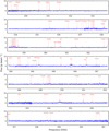 |
Fig. 1 Spectrum towards N63, at the continuum peak. The brightest lines are marked and labelled. |
2.4 Self calibration and imaging
The sources observed here are all relatively strong continuum sources (peak intensities range from 0.25 to 1.66 Jy beam−1; Table 3). Thus, self calibration was attempted iteratively on each source in order to further lower the noise levels. This was achieved by first identifying the line-free channels by eye in order to isolate the continuum emission. Next, phase-only gain solutions were attempted first in solution intervals of 240 s, and from there going progressively down to intervals of 60s. If a gain solution failed, the previous step was kept as the optimal solution. The self calibration typically improved the noise level by a factor of three, from ∼ 1.5 × 10⁻² to ∼5.0 × 10⁻³ Jy beam−1 for the continuum data. The self-calibration solution obtained from the continuum data was then applied to the entire cube. The continuum emission was subtracted from each chunk separately.
The next step was to image the complex visibilities. This was done by defining a circular clean mask centred on each source, (or a central point between continuum cores), and including all continuum cores. The Briggs ‘robust’ parameter was set to 2, corresponding to a natural weighting of the visibilities. This optimises for sensitivity at the cost of angular resolution. The resulting beam size was typically ∼1″.5 (~2000 AU at a source distance of 1.3 kpc) and rms noise levels of around 0.3 Jy beam−1 in each 0.48 km s−1 channel (see van der Walt et al. 2021, for further details). The resulting noise levels and beams are reported in Table 3.
The maximum recoverable scale (MRS) of the observations is calculated using equation MRS = 1.22 × λ/D, where λ is the wavelength of the observations and D the shortest distance between two antennae (shortest baseline) of the interferometer. With λ = 870 µm (345 GHz) and D = 16 m, an MRS of ∼14″, or ∼20 000 AU at a distance of 1.3 kpc is obtained. This scale almost corresponds to the sizes of the envelopes (Pitts et al. 2022). Similarly, the field of view (FoV) is ∼36″ ∼50 000 AU. There will therefore be some resolving-out, but this has not prevented a quantitative analysis before (e.g. Jørgensen et al. 2007; Lee et al. 2015; Stephens et al. 2018).
PILS-Cygnus continuum source properties.
3 Results
3.1 Continuum emission
The PILS-Cygnus source sample is listed in Table 1. N30 was analysed in detail in van der Walt et al. (2021), with 345 GHz (∼870 µm) continuum emission maps for the remaining nine sources shown in Fig. 2; these maps were first presented in Pitts et al. (2022). We note that N54 is shown together with N53, as they fall within the same field of view.
Five of the ten sources are located in the dense DR21 ridge N53, N54, N51, N38 and N48 (d = 1.5 kpc; see also Fig. 3), where several filaments intersect (see e.g. Motte et al. 2007; Reipurth & Schneider 2008; Pitts et al. 2022). N30, N12 and N63 are located to the north, west and south of DR21, respectively (d = 1.3–1.4 kpc). The two remaining sources, S26 and S8, are located in the southern Cygnus-X molecular cloud, with S26 likely not being directly associated with Cygnus-X (d = 3.3 kpc for S26, and 1.4 kpc for S8).
The first panel in Fig. 2 shows S26, which is a single source at the ~1″.5 resolution of the PILS-Cygnus observations. There is some extended emission to the north-east of the emission peak, as well as some extended emission ∼5″ to the northwest, independent of the emission peak. The two other northern sources, N12 and N63 are shown in the second panel and first panel of the second row, respectively. N12 shows two cores at ∼1″. 5 resolution, with some extended emission to the northwest, while N63 is singular, but with extended emission to the south-east.
Of the DR21 sources, N53 has two components at the resolution of the PILS-Cygnus observations, with spiralling extended emission connecting the two cores. N54 is shown in the same panel as N53, with a separation of ∼10″ between the two sources. N51 is shown in the first panel of the third row, with N38 in the second panel. Both sources show large structure in extended emission, to the northwest of N51, and south of N38, with two faint cores north and northwest of N38. The first panel of the bottom row shows N48, with this source consisting of three elongated and connected cores, with large structure in extended emission surrounding these cores. The second panel of the bottom row shows S8, which consists of two cores, with four fainter cores to the south.
The molecular outflows may impact the observed emission, either through excitation (some molecules will more readily be excited in the dense and warm gas in outflows) or chemistry (sputtering and gas-phase reactions may lead to abundances of some molecules increasing dramatically). The sources all show outflow activity as traced by CO 3–2 emission (Skretas & Kristensen 2022). The directions and extent of the outflows are shown in the continuum maps with red and blue arrows, for easy comparison with the observed molecular emission described below. Furthermore, a number of sources show SiO 8–7 emission, another shock and outflow tracer. The SiO emission tends to be more compact, and less extended than the CO emission (≲a few arcsec, Skretas & Kristensen 2022).
Furthermore, UV radiation from the nearby OB associations may affect the chemistry observed towards these sources. For this reason, the direction of the nearest OB associations (in the plane of the sky) are also marked on the continuum maps. For the northern sources, the OB association the closest by is OB2. The typical projected distance to the sources is ~45 pc, for an average distance of 1.4 kpc.
Finally, the dust may act to shield the molecular emission from the protostars, if the dust is optically thick. To evaluate if the dust itself is optically thick to molecular emission, we follow the recipe outlined in, for example van der Walt et al. (2021), whereby we assume a dust temperature of 30 K and a gas-to-dust mass ratio of 100. We calculate the total mass of gas and dust using the following standard relation:
 (1)
(1)
where Sv is the peak intensity of the source, d the distance, and Bν(T) the Planck function at specific frequency and temperature. We used a dust opacity κν = 0.0175 cm2 per gram of gas for a gas-to-dust ratio of 100 (at frequency ν = 345 GHz; Ossenkopf & Henning 1994). We calculate and list the resulting mass of gas and dust for each source in Table 3 for Τ = 30 K. An average dust temperature may be low, particularly for sources such as N30 and S26 where the 100-K radius is similar to the beam (Table 3). If a larger temperature is used, the mass decreases. For the specific example of a temperature of 100 K, the total mass would be lower by a factor of 4.
The optical depth can then be calculated as (e.g. Schöier et al. 2002):
 (2)
(2)
where µ = 2.8 is the mean molecular weight used, which also accounts for Helium (Kauffmann et al. 2008), mH the mass of the Hydrogen atom, and  the H2 column density (see also van der Walt et al. 2021). The dust opacities (Table 3) are found to be <0.5 for all but two sources: S26 and N63. For these sources, the dust opacities are 1.02 and 0.58, respectively. Specifically for S26, the source breaks into three continuum sources when observed at higher angular resolution, but the molecular emission appears to be extended beyond these continuum peaks (Suri et al. 2021). This suggests that although the continuum emission is moderately optically thick, it does not shield the bulk of the molecular emission. For the case of N63, the source appears to be very compact and most of the mass is contained within a radius of ~2500 AU (Duarte-Cabral et al. 2013). Thus, it may very well be that if the source was observed at higher angular resolution, the dust opacity would increase. However, we do not have the data to validate this hypothesis, and we conclude that the dust may be slightly optically thick towards N63. Moreover, if the dust temperature is larger than 30 K, and the masses thus are lower, the dust opacities will also be lower and should therefore be considered as upper limits here. For the other sources, dust opacity will not play a role on the scales observed here.
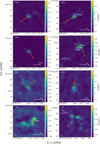 |
Fig. 2 Continuum images for the PILS-Cygnus source sample. We note that N53 and N54 are shown in the same image. The crosses mark the brightest core and the position at which the spectrum for each source was extracted, while the plusses mark the central position between the red-and blue-shifted CO emission lobes. |
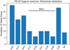 |
Fig. 3 Number of molecules and their isotopologues detected in each source, grouped by region and with the DR21 sources labelled. |
3.2 Molecular line emission
The molecular detection statistics for the source sample are shown in Table 4, with the number of molecules and their isotopologues detected towards each source shown in Fig. 3. N30 and S26 have 30 and 28 molecular detections, respectively. Towards N63, 22 molecular species are detected, with 19 detected towards N12. For the DR21 sources ten molecular species are detected towards N53, N51 and N38, and six are detected towards both N54 and N48. Nine molecular species are detected towards S8.
Line identification was performed following the process described in van der Walt et al. (2021), which follows the points laid out by Snyder et al. (2005) and using the spectral modelling package CASSIS2 (Vastel et al. 2015) to construct a synthetic spectrum covering the frequency range of the PILS-Cygnus observations (329–361 GHz) using the molecular spectroscopy data from the CDMS3 (Müller et al. 2001, 2005; Endres et al. 2016) and JPL4 (Pickett et al. 1998) databases. The synthetic spectra were constructed by first adding previously identified molecules and comparing with the observed spectra to find and identify all lines with intensity above 3σ, where σ is the noise level of the observed spectrum.
Spectra and molecular maps are shown for the source N63 in Figs. 1 and 4, respectively, with the molecular transitions used to produce the molecular maps listed in Table 5. Where more than one transition for a given molecule were detected, the lines were stacked following the methodology outlined in van der Walt et al. (2021). Figures and tables for the source sample are presented in Appendix A.
Observed line plots of the CASSIS synthetic spectral lines over-plotted on the observed lines for each source are shown in Appendix C, with the full line lists of observed lines above 3 σ for each source in Appendix D. Appendices are available online at Zenedo.org.
3.3 Emission morphology
The emission of strong lines of each detected species was mapped and is shown in Figs. A.9–A.16. We generally identify four different types of emission morphology: (i) emission that appears unresolved and peaks on the continuum source; (ii) emission that appears unresolved but offset from the continuum source; (iii) resolved (extended) emission that peaks on the continuum source; and finally (iv) resolved emission that peaks offset from the source. Emission from the detected species is classified according to this scheme and based on a by-eye inspection of each map, with the classification shown in Table 4.
It is difficult to see a pattern in the emission morphology. The only constant is that the emission from the most simple carbon-bearing molecules (CO, HCO+, HCN, and CS and their isotopologues) appears to be extended. Emission from COMs, on the other hand, appears to be both compact and extended, when detected, as for example seen towards N63 (Fig. 4).
van der Walt et al. (2021) noted that the molecular emission towards N30 was offset from the continuum source. Particularly, they found that this offset was independent of excitation, that is it was independent of the upper-level energy of the observed transition and the critical density of the transition. The same is seen for the other sources observed here: for the molecules where several bright transitions are detected, these all peak in the same place independent of excitation. This suggests that any difference in spatial extent of emission is caused by chemistry and not excitation.
Detection statistics for the PILS-Cygnus sources.
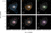 |
Fig. 4 Molecules observed towards N63. The contour levels for both the continuum (grey dashed lines) and molecular emission (coloured) are 3, 6, 12, 24 and 48σ. The pluses are the molecular emission peak positions derived from 2D Gaussian fits (Table 5), and these are colour-coded according to molecule. |
3.4 Column densities
Column densities and excitation temperatures are derived for the observed molecules towards each source. Following the procedure described in van der Walt et al. (2021), we constructed a synthetic spectrum with CASSIS, using only line emission and assuming local thermodynamic equilibrium (LTE). The best-fit spectral model for each molecule was found by computing the reduced χ2 minimum using the inbuilt regular grid function in CASSIS and covering a large parameter space. The free parameters used in the fit were source velocity (vsource), the full width half maximum (FWHM), the column density (N), and excitation temperature (Tex). The FWHM and vource were estimated by fitting a Gaussian profile to a few unblended lines, which were then used in a parameter space of 4 km s−1 around the line, in steps of 0.5 km s−1 (approximately the channel width). Initially, a large parameter space was used for N with Nmin = 1014 cm−2 and Nmax = 1019 cm−2 and ten logarithmically spaced steps in this range, while for Tex a minimum of 90 K and a maximum of 300 K was used, also with ten steps in between these values. The parameter ranges were then reduced by running a few iterations, while keeping the steps larger than the uncertainties for each parameter. Throughout the modelling process the source sizes were assumed to be ∼1″.5, comparable to the beam size of the PILS-Cygnus observations. The derived values for N63 are shown in Table 6, with the source sample column densities presented in Appendix B, together with the abundances relative to CH3OH shown in Fig. B.1.
The uncertainties on N and Tex were estimated as follows: first N (or Tex) is fixed and then Tex (or N) is adjusted until the result of the change on the fit can be seen (method described by Calcutt et al. 2018). This is shown in parenthesis after the values for N and Tex in Tables B.1–B.8.
In cases where molecular lines are optically thick, isotopo-logues of the molecule were used and multiplied by the local ISM ratios: 12C/13C ∼68 (Milam et al. 2005), 32S/34S ∼22 and 16O/18O ∼560 (Wilson & Rood 1994). For CH3CN the higher vibrational transition v8 = 1 was used, since no isotopologues of CH3CN were detected. Finally, for sources where no isotopo-logues of CH3OH or SO were detected we give lower limits for these molecules, derived by fixing Tex to typical values and fitting the synthetic spectrum to the observed lines. The lower limit reflects that the emission from these molecules is likely optically thick.
The resulting column densities are represented as relative abundances in Figs. 5−7 for three representative species. These species were chosen as a shock/outflow tracer (SO), a hot-core tracer (CH3CN), and the most commonly observed COM (CH3OH) (e.g. Tychoniec et al. 2021). From Fig. 5 we see that the relative abundances of CH3CN-to-CH3OH do not exhibit a noticeable trend, whereas relative abundances of SO-to-CH3OH (Fig. 6) seem to generally increase with luminosity, while CH3CN-to-SO (Fig. 7) abundances seem to decrease with luminosity. However, with only four data-points, this result needs to be confirmed, which ideally would include more observations of sources from the same cloud.
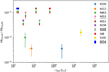 |
Fig. 5
|

4 Discussion
4.1 Cold chemistry
The outer regions of the source envelope and the molecular outflows are traced by simple molecules. CO is a good tracer for the source outflows on a large scale, while its isotopologues, 13CO, C18O and C17O are less abundant and trace the source disc and envelope (e.g. Jørgensen et al. 2002). Other simple molecules are SO, CS, CN, HCN and HCO+ and they are dense gas tracers (Jørgensen et al. 2004b), tracing the source outflows, cavity walls, disc and envelope (see also Tychoniec et al. 2021, for a review on which molecules traces which part of the physical environment of protostellar sources). At large scales, these simple molecules are detected towards all sources in the sample and the environment surrounding the source envelopes does not seem to play a role in setting their abundances.
Figures 8–10 show the intensity ratios of the CO, 13CO and C18O lines to the peak continuum emission for each source. The continuum emission scales with the dust mass, for a given temperature, and thus the total mass for a given gas/dust ratio. When averaged over the area, in this case a beam, it becomes directly proportional to the total (H2) column density. Similarly, under the assumption of optically thin emission, the line emission is directly proportional to the column density of the upper energy level. Adding the assumption of LTE, this can be scaled to the total column density of the molecule for a given excitation temperature. For molecules and transitions with low critical density compared to the density of the surroundings, which is the case for CO and its isotopologues, the level populations are likely to be in LTE. Thus, to a first order, this ratio reflects the CO abundance in the gas.
For the figures showing 13CO and C18O, we have multiplied the intensities with the typical ISM ratios for 12C/13C and 16O/18O (68 and 560, respectively, Wilson 1999) to turn them into proxies for the 12CO abundance. These ratios are shown with respect to the bolometric luminosity for each source. From the figures it can be seen that the CO and 13CO lines appear to be optically thick as we would expect, since the three figures should show similar ratios if this was not the case. Therefore Fig. 10 can be taken as a more accurate representation of the CO abundance. Figure 10 demonstrates that the CO abundance seems to be relatively constant with respect to bolometric luminosity, with values within a factor of two, with a mean (excluding N63) of 3.0 × 10³ and standard deviation 1.2 × 10³, whereas source luminosities vary between 102 and ~2× 10⁵. The only exception is N63 with a low CO gas abundance (a factor of 7 lower than the mean). This source has a high peak continuum emission compared to the other sources (1.66 Jy beam−1 compared to ~0.4 Jy beam−1 for the other sources), while it has a low luminosity (~3 × 10²). This suggests that N63 is a colder source, but with a more massive core at the small scales that we observe.
One caveat is that an interferometer such as the SMA, will spatially filter emission from large scales and not detect this emission. For the observations presented here, the maximum recoverable scale is ~14″ or 2×10⁴ AU at the distance of Cygnus. This scale corresponds to the typical envelope size of these sources (Pitts et al. 2022), and so is not expected to be a dominant factor. Furthermore, we are here primarily concerned with the dense inner envelope, which does appear in both dust continuum and CO isotopologue emission. In this respect, we follow previous studies (e.g. Jørgensen et al. 2007; Lee et al. 2015; Stephens et al. 2018).
Overall, however, it is clear that the abundance of the simplest molecules observed in this survey do not vary significantly between the different sources. This suggests that the very simple chemistry is independent of the environment and the location with respect to both the OB2 association and the DR21 filament.
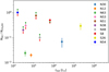 |
Fig. 6
|

Column densities, excitation temperatures, FWHM and vpeak derived at the continuum peak position of N63.
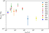 |
Fig. 7
|

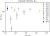 |
Fig. 8 CO to dust ratio vs bolometric luminosity. |
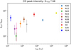 |
Fig. 9 CO to dust ratio (derived from 13CO) vs bolometric luminosity. |
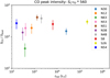 |
Fig. 10 CO (derived from C18O) to dust ratio vs bolometric luminosity. |
4.2 Hot core chemistry
The warm inner regions (temperatures ≳ 100 K) of protostars are observed at high resolution, with COMs tracing these regions (hot cores). This is because in these warm regions the molecular ices residing on the dust grains are thermally desorbed into the gas phase (e.g. Herbst & van Dishoeck 2009). As a consequence, hot core regions are often traced by molecules that formed directly on the grains and then stay on the grains, such as methanol, CH3OH, until they thermally sublimate.
CH3OH is observed towards or close to all the sources in this work. CH3OH is a common molecule observed towards protostars, but is also observed in outflows, as molecules frozen out on dust grains are sputtered off the grains into the gas phase (e.g. Suutarinen et al. 2014), as well as the surface regions of protostellar discs as material falls onto the disc and the dust is heated up to release the molecules frozen out (e.g. Csengeri et al. 2019). For the source sample in this survey it seems to be a combination of these processes that is observed (see also van der Walt et al. 2021). 13CH3OH and CH3CN are detected towards only four sources, N30, N12, S26 and N63, and CH3OCH3 and CH3OCHO are detected towards N30, S26 and N63. The lack of COM detections towards the other sources could be because the observations are sensitivity limited towards these sources. To check this hypothesis, we calculate the relative molecular abundances N(CH3OCHO)/N(CH3OH) towards N30, S26 and N63 where we detect CH3OCHO and compare with N12 where this molecule is not detected. For N30, S26 and N63, a value of ~0.02 is obtained, which, when turned into an emission spectrum, is consistent with the noise level for N12, suggesting that the observations are indeed sensitivity limited. This result is further corroborated by the 100 K radii for the sources listed in Table 3. The 100 K radius for all sources, except N30 and S26, falls well within the beam size of the PILS-Cygnus observations, and any hot core emission is likely severely beam diluted.
As illustrated in the case of N30, a ‘hot core’ is not necessarily a hot core. Towards N30 the COM emission is found to be extended and offset from the location of the continuum positions, suggesting that the emission originates from a region where thermal desorption is not the dominant desorption mechanism. Instead, it seems more plausible that the emission originates in a rotating disc-like structure (van der Walt et al. 2021). This type of hot-core emission that is not caused by thermal desorption of molecules is seen towards more and more sources (e.g. Avery & Chiao 1996; Jørgensen et al. 2004b; Arce et al. 2008; Sugimura et al. 2011; Podio et al. 2015; Drozdovskaya et al. 2015; Lefloch et al. 2017; Orozco-Aguilera et al. 2017; Artur de la Villarmois et al. 2018; Csengeri et al. 2018, 2019). Of the sources observed here, S26 seems to be a classical hot core at the scales we observe, but at higher angular resolution it is fragmented (Jiménez-Serra et al. 2012; Suri et al. 2021), which suggests that a more complicated morphology for the COM emission would be observed with higher angular resolution observations. N12 reveals two continuum cores at the resolution of the PILS-Cygnus observations, with COM emission peaking towards the MM2 core. However, from the emission map of CH3OH in Fig. A.10 it can be seen that there is another CH3OH peak to the north-west of the continuum cores, and along the CO outflow axis, suggesting this emission peak is due to sputtering caused by the outflow. This is not seen in the emission from other COMs. N63 shows only a single core at the angular resolution of the PILS-Cygnus observations, but with significant extended emission along the CO outflow direction seen in CH3OH and to a lesser extent SO (Fig. 4). Again, this suggests that at least some emission is outflow-related.
The extent of the COM emission, when detected, does not appear to correlate with the direction to the OB2 association. This result is based on very few sources (N12, N30, and N63), and so is not enough to draw strong conclusions. However, it appears that on the small scales observed here, the COM emission is not strongly affected by the external UV radiation. On larger, envelope scales, the external environment may play a larger role.
Of the sources observed here, four harbour known compact H II regions: S26, N30, S8, and N51 (Lynds 1965; Haschick et al. 1981; Torrelles et al. 1997; Grasdalen et al. 1983). Two of these also show COM emission (S26 and N30). In the evolutionary scheme proposed by Motte et al. (2018), the hot cores are the largest right before the sources develop H II regions. This suggests that these two sources, S26 and N30, are relatively evolved sources, and that protostellar evolution likely plays an important role in setting the complex chemistry. Similarly, S8 and N51 might have H II regions large enough that the hot cores are diminishing in size and not detectable to us, making them even more evolved. In this evolutionary scheme, the two other sources with COM emission, N12 and N63, would be at a stage prior to developing detectable H II regions, and the remaining sources would be at earlier evolutionary stages where the hot cores are not developed yet. We emphasise that in the absence of clear evolutionary tracers, this scenario is hypothetical.
The chemistry observed towards the four “hot cores” also does not seem to be affected by the external environment. When comparing the CH3OH column density to the CH3CN column density for the four sources (Fig. 5), the ratio is within a factor of five (with a mean of =8.5 × 10⁻³ and standard deviation =5.4 × 10⁻³). This again suggests, albeit based on a very small number of sources, that the external environment plays a small role in setting the chemistry.
The value of the column-density ratio N(CH3CN)/ N(CH3OH) ranges from 4 × 10⁻³ to 1.7 × 10⁻² (Fig. 5). The lower values are similar to the results of the PILS survey of IRAS16293–2422B (4.0 × 10⁻³; Jørgensen et al. 2016) and lower than that of Sgr B2(N2) (5.5 × 10⁻²; Belloche et al. 2016); the upper limits are consistent with both values and not particularly sensitive. Garrod et al. (2022) suggest that this difference is caused by the length of the warm-up phase, where a slower warm-up phase leads to a higher column-density ratio, and vice versa. In turn, that would suggest that the warm-up phases for these protostars are more closely related to that of IRAS16293, as opposed to Sgr B2(N2).
Interestingly, the formation paths of CH3OH and CH3CN may be different. It is generally accepted that CH3OH forms from hydrogenation of CO frozen out on icy dust grains. CH3CN, on the other hand, likely forms in the gas phase in hot cores (Garrod et al. 2022) as a second-generation molecule (Herbst & van Dishoeck 2009). Thus, to a first order, there is no a priori expectation that the two species should correlate in column density. Furthermore, since CH3CN forms in dense, warm gas, the expectation is that emission is compact and peaks on the continuum position. This is indeed the case for S26. For N30, emission is extended and peaks off-source (van der Walt et al. 2021), whereas for N12 emission is extended and also peaks off-source. In this case, higher-angular resolution observations would be required to precisely pinpoint the origin of both CH3OH and CH3CN.
To further shed light on the origin of CH3OH and CH3CN, their column densities are compared to that of SO. SO is often used as an outflow tracer (e.g. Tabone et al. 2017; Artur de la Villarmois et al. 2018; van Gelder et al. 2021), and generally traces warm gas. We do not find any signs of outflow activity in the line profiles of SO, but it is possible that this molecule traces accretion shocks onto a disc (Artur de la Villarmois et al. 2018), in which case the line profile would not show strong line wings or asymmetries. The column density ratio N(SO)/N(CH3OH) may show a weak increase with luminosity, but with only four data-points it is not possible to draw any strong conclusions regarding trends with luminosity. Towards these sources, accretion shocks may be stronger (impacting higher-density material at higher velocities), in which case the SO abundance is expected to increase by orders of magnitude (van Gelder et al. 2021). Furthermore, the models do not predict an enhanced CH3OH abundance, and so it is expected that the ratio of N(SO)/ N(CH3OH) increases with increasing strength of the accretion shock. To test this scenario further, deeper observations at higher angular resolution are needed, and these should be able to constrain the SO2 column density; the models make further predictions regarding the SO/SO2 column density ratio, that will be used for constraining the model. Furthermore, more data-points will clearly be needed.
4.3 Deuteration
We detect low levels of deuteration towards N30, N12, N63 and S26, with N12 and N63 having slightly higher levels than N30 and S26. No deuterated molecules are detected towards the remaining sources of the sample. HDO is detected towards N30, S26, N12 and N63, while CH2DOH is detected towards N63, and is very tentatively present towards N12, however only a ∼2σ peak can be found in this work. The D/H ratios are derived for N(CH2DOH)/N(CH3OH), after correcting for the three symmetries of the CH2DOH molecule (see e.g. Jørgensen et al. 2018; Manigand et al. 2019), towards N63 of ∼1%, with upper limits for N30 and S26 of ∼0.1% and ∼0.3%, respectively, and with an upper limit for N12 of ∼1%. The higher D/H ratio derived for N63 is expected, since this source seems to be a cold source, as discussed in Sec. 4.1 above (see also discussion in Duarte-Cabral et al. 2013). The colder the source is, the more efficient the deuteration chemistry should be (e.g. Ceccarelli et al. 2007; Caselli et al. 2019), which leads to an increase in the deuteration fraction in molecules such as CH3OH. An alternative explanation would be that it is a low-mass source, with a longer cold phase, such that even if the deuteration chemistry runs less efficiently, it has longer time to work, leading to the same result. However, given the high continuum emission peak (1.66 Jy beam−1; Table 3), it suggests that this is a cold, dense and massive source (we also note in Table 3 that N63 has a mass of >10 M⊙). With a higher level of CO freeze out than the other sources, it suggests this source formed at a cooler temperature (<30K), where deuterium reactions are more efficient (Taquet et al. 2014; Bøgelund et al. 2018). More observations are necessary to confirm this result.
N30 and S26 compare well with other high-mass sources, (for example Orion KL has values around 0.2–0.8% while Sgr B2 (N2) has a D/H ratio of 0.12% for CH2DOH; Neill et al. 2013; Belloche et al. 2016). N12 and N63 have a D/H ratio slightly higher than high-mass sources, but still a factor of two or three lower than low-mass sources such as IRAS 16293–2422 B (with D/H ratios of 2–3%; Jørgensen et al. 2018). Thus, the deuteration fraction seems to be very sensitive to changes in the local environment, as expected (Manigand et al. 2019; Jensen et al. 2021).
4.4 External environment
As discussed in Sect. 3.1 above, UV radiation from bright stars can affect the observed chemistry of newly formed stars. A strong background radiation field may heat up the environment making the formation of molecules on dust grains inefficient, since the higher temperatures will prevent the precursor molecules (e.g. CO) from freezing out onto the dust grains, and thus not participate in the further formation of COMs. Higher formation temperatures also result in lower deuteration, since deuterium reactions are inefficient at temperatures >30 K (see e.g. Taquet et al. 2014; Bøgelund et al. 2018).
Of the ten sources, eight are located at distances between 30–50 pc to the CygX-OB2 association. Five of these sources (N53, N54, N51, N38 and N48) are located in the DR21 ridge, and these sources show similar chemistry at the sensitivity of our observations, that is, we detect few COMs towards these sources. The three sources that surround DR21 (N30, N12 and N63) all have a higher amount of COM detections, with N63 and N12 also having a higher D/H ratio than the other sources. N12 and N63 are both closer to CygX-OB2 than the DR21 sources. The remaining two sources are S26, which is located at ∼3.3 kpc, too far from CygX-OB2 for it to have any effect, and S8 with a high uncertainty in its distance (>80 pc from CygX-OB2).
The lack of COM detection in the DR21 ridge (and COM detections towards N30, N12 and N63) seems to suggest that the external environment does not play a noticeable role in the formation of COMs in this region and that the local environments surrounding the protostars play a bigger role. On the other hand, as discussed above, our observations are probably sensitivity limited (Sect. 4.2), implying that follow-up observations are required to confirm this speculation. The sensitivity limit was estimated using N(CH3OH) as a reference frame.
The five sources in the DR21 ridge represent something of a conundrum. The sources have the lowest masses in the sample, inferred from the 870 µm fluxes, and the natural conclusion would be that this is consistent with low masses of the hot cores, and thus low column densities of COMs. On the other hand, the sources do not have the lowest luminosities. This means that the radii of the hot-core regions should be relatively large, and more mass should be included in the hot-core region, which should lead to higher COM column densities and detections. In this case, it appears as if the lower mass is the dominating factor since no COM emission is detected towards the sources, consistent with lower CH3OH column densities towards these sources (Sect. 4.2). The relatively high luminosity compared to the mass, can likely be attributed to on-going accretion from the DR21 ridge onto these sources (Pitts et al. 2022). This in turn suggests that the environment does play a role, in the sense that it matters whether sources form in dense molecular ridges (‘hubs’) or not in terms of our ability to detect COM emission. However, whether this is reflected in the chemistry or not is an open question.
Observations of low-mass protostellar sources appear to suggest that the difference in location, specifically inside or outside a filament or ridge, plays a role in setting the chemistry. The ‘Astrochemical Surveys At IRAM’ (ASAI; Lefloch et al. 2018) programme find that sources located in filaments appear to have a hot-core chemistry, that is the organic chemistry is dominated by C-O-bearing molecules. On the other hand, sources located outside dense filaments tend to show a chemistry dominated by C-C-bearing molecules, that is the so-called warm carbon-chain chemistry (WCCC). This result is based on observations of between four and five sources in each category as observed with a single-dish telescope. Interferometric observations reveal that on small scales, WCCC sources may be dominated by a hot-core chemistry (e.g. Oya et al. 2019), making the picture less clear. Thus, to fully address how the location, inside our outside a filament, affects the chemistry, deeper observations spanning a range of spatial scales is required for a large sample.
4.5 Morphology
From the observations presented here and in van der Walt et al. (2021) it can be seen that the origin of COMs detected in and near star-forming regions is a combination of thermal (the classical hot core scenario) and non-thermal (sputtering caused by outflows and accretion of inflowing material onto a disc structure) processes. The emission morphology of the PILS-Cygnus sources seem to point to hot cores at small scales, with COMs also detected in the surrounding envelope and outflows. We know that different molecules trace different regions of the protostar (e.g. Herbst & van Dishoeck 2009; Tychoniec et al. 2021), which make studies like PILS-Cygnus so valuable, where a large frequency range are covered at high resolution, making it possible to observe a large amount of COM transitions and in an unbiased way. This results in a more complete picture of the morphology of star-forming regions.
5 Summary and conclusions
This paper presents the source sample and results of the PILS-Cygnus survey. Ten intermediate- and high-mass sources were observed with the SMA, all located in the nearby Cygnus-X star-forming region. The observations were done at ∼1″.5 resolution (∼2000 AU), and span the entire frequency range of 329–361 GHz. The main results of the survey can be summarised as follows:
Continuum and line emission is detected towards all sources; the line emission is from small species, such as CO, H2CO, CS, and HCO+. The abundance of CO appears constant over all species, with only one exception, indicating that the chemistry of this simple molecule does not vary over the cloud;
Emission from the simplest complex organic molecule, methanol, CH3OH, is detected towards nine sources, and is found to trace the hot core, the outflow, other shock activity, or a combination of these. This in turn implies that some ‘hot cores’ are not only caused by thermal desorption but are, at least partly, due to shocks;
Emission from more complex species, for example CH3OCH3 and CH3OCHO, is detected towards 3 sources, and typically originates in the hot core. CH3CN is detected towards one additional source. Column densities have been inferred for all sources and species, and the lack of detection of more complex organic species is set by the sensitivity;
Deuterated methanol, CH2DOH, is firmly detected towards one source. The deuteration fraction for this source is high, ∼1%, suggesting that this source either is cold now (T < 30 K) or has been so for an extended period in the past, whereas the other nine sources have not;
There are no apparent differences between the sources in terms of chemistry as a function of distance to the OB2 association, nor location within the DR21 filament. This suggests, although based on a small number of sources, that the external environment only plays a minor role in shaping the chemistry and its associated evolution of these sources. Instead, local factors such as the thermal history and outflows, appear more important for the observed chemistry.
With these observations, characterisation of molecular emission from intermediate- and high-mass protostellar sources in Cygnus-X is started. The observations demonstrate the usefulness and necessity for observing a large frequency range in order to properly understand the chemistry of such complex objects. Finally, the initial results presented here indicate that the external environment only plays a minor role in setting the chemistry on smaller scales (∼2000 AU), but clearly more observations are needed to verify this statement.
Acknowledgements
We acknowledge and thank the staff of the SMA for their assistance and continued support. The authors wish to recognise and acknowledge the very significant cultural role and reverence that the summit of Mauna Kea has always had within the indigenous Hawaiian community. We are most fortunate to have had the opportunity to conduct observations from this mountain. The research of SJvdW and LEK is supported by a research grant (19127) from VILLUM FONDEN. The research of HC is supported by an OPUS research grant (2021/41/B/ST9/03958) from the Narodowe Centrum Nauki.
References
- Arce, H. G., Santiago-García, J., Jørgensen, J. K., Tafalla, M., & Bachiller, R. 2008, ApJ, 681, L21 [NASA ADS] [CrossRef] [Google Scholar]
- Artur de la Villarmois, E., Kristensen, L. E., Jørgensen, J. K., et al. 2018, A&A, 614, A26 [NASA ADS] [CrossRef] [EDP Sciences] [Google Scholar]
- Avery, L. W., & Chiao, M. 1996, ApJ, 463, 642 [NASA ADS] [CrossRef] [Google Scholar]
- Belloche, A., Müller, H. S. P., Garrod, R. T., & Menten, K. M. 2016, A&A, 587, A91 [NASA ADS] [CrossRef] [EDP Sciences] [Google Scholar]
- Belloche, A., Maury, A. J., Maret, S., et al. 2020, A&A, 635, A198 [NASA ADS] [CrossRef] [EDP Sciences] [Google Scholar]
- Bisschop, S. E., Jørgensen, J. K., van Dishoeck, E. F., & de Wachter, E. B. M. 2007, A&A, 465, 913 [NASA ADS] [CrossRef] [EDP Sciences] [Google Scholar]
- Bøgelund, E. G., McGuire, B. A., Ligterink, N. F. W., et al. 2018, A&A, 615, A88 [Google Scholar]
- Calcutt, H., Jørgensen, J. K., Müller, H. S. P., et al. 2018, A&A, 616, A90 [NASA ADS] [CrossRef] [EDP Sciences] [Google Scholar]
- Caselli, P., Sipilä, O., & Harju, J. 2019, Philos. Trans. Roy. Soc. Lond. A, 377, 20180401 [NASA ADS] [Google Scholar]
- Ceccarelli, C., Caselli, P., Herbst, E., Tielens, A. G. G. M., & Caux, E. 2007, in Protostars and Planets V, eds. B. Reipurth, D. Jewitt, & K. Keil, 47 [Google Scholar]
- Cesaroni, R., Hofner, P., Araya, E., & Kurtz, S. 2010, A&A, 509, A50 [NASA ADS] [CrossRef] [EDP Sciences] [Google Scholar]
- Codella, C., Ceccarelli, C., Caselli, P., et al. 2017, A&A, 605, L3 [NASA ADS] [CrossRef] [EDP Sciences] [Google Scholar]
- Csengeri, T., Bontemps, S., Wyrowski, F., et al. 2018, A&A, 617, A89 [NASA ADS] [CrossRef] [EDP Sciences] [Google Scholar]
- Csengeri, T., Belloche, A., Bontemps, S., et al. 2019, A&A, 632, A57 [NASA ADS] [CrossRef] [EDP Sciences] [Google Scholar]
- Drozdovskaya, M. N., Walsh, C., Visser, R., Harsono, D., & van Dishoeck, E. F. 2015, MNRAS, 451, 3836 [NASA ADS] [CrossRef] [Google Scholar]
- Duarte-Cabral, A., Bontemps, S., Motte, F., et al. 2013, A&A, 558, A125 [NASA ADS] [CrossRef] [EDP Sciences] [Google Scholar]
- Endres, C. P., Schlemmer, S., Schilke, P., Stutzki, J., & Müller, H. S. P. 2016, J.Mol. Spectrosc., 327, 95 [NASA ADS] [CrossRef] [Google Scholar]
- Garrod, R. T., Jin, M., Matis, K. A., et al. 2022, ApJS, 259, 1 [NASA ADS] [CrossRef] [Google Scholar]
- Goicoechea, J. R., Pety, J., Gerin, M., et al. 2006, A&A, 456, 565 [NASA ADS] [CrossRef] [EDP Sciences] [Google Scholar]
- Grasdalen, G. L., Gehrz, R. D., Hackwell, J. A., Castelaz, M., & Gullixson, C. 1983, ApJS, 53, 413 [NASA ADS] [CrossRef] [Google Scholar]
- Haschick, A. D., Reid, M. J., Burke, B. F., Moran, J. M., & Miller, G. 1981, ApJ, 244, 76 [NASA ADS] [CrossRef] [Google Scholar]
- Herbst, E., & van Dishoeck, E. F. 2009, ARA&A, 47, 427 [NASA ADS] [CrossRef] [Google Scholar]
- Jensen, S. S., Jørgensen, J. K., Kristensen, L. E., et al. 2021, A&A, 650, A172 [EDP Sciences] [Google Scholar]
- Jiménez-Serra, I., Zhang, Q., Viti, S., Martín-Pintado, J., & de Wit, W. J. 2012, ApJ, 753, 34 [Google Scholar]
- Jørgensen, J. K., Schöier, F. L., & van Dishoeck, E. F. 2002, A&A, 389, 908 [CrossRef] [EDP Sciences] [Google Scholar]
- Jørgensen, J. K., Hogerheijde, M. R., Blake, G. A., et al. 2004a, A&A, 415, 1021 [NASA ADS] [CrossRef] [EDP Sciences] [Google Scholar]
- Jørgensen, J. K., Schöier, F. L., & van Dishoeck, E. F. 2004b, A&A, 416, 603 [Google Scholar]
- Jørgensen, J. K., Bourke, T. L., Myers, P. C., et al. 2007, ApJ, 659, 479 [Google Scholar]
- Jørgensen, J. K., van der Wiel, M. H. D., Coutens, A., et al. 2016, A&A, 595, A117 [Google Scholar]
- Jørgensen, J. K., Müller, H. S. P., Calcutt, H., et al. 2018, A&A, 620, A170 [Google Scholar]
- Kauffmann, J., Bertoldi, F., Bourke, T. L., Evans, N. J. I., & Lee, C. W. 2008, A&A, 487, 993 [NASA ADS] [CrossRef] [EDP Sciences] [Google Scholar]
- Kryukova, E., Megeath, S. T., Gutermuth, R. A., et al. 2012, AJ, 144, 31 [Google Scholar]
- Kryukova, E., Megeath, S. T., Hora, J. L., et al. 2014, AJ, 148, 11 [Google Scholar]
- Kurtz, S., Cesaroni, R., Churchwell, E., Hofner, P., & Walmsley, C. M. 2000, in Protostars and Planets IV, eds. V. Mannings, A. P. Boss, & S. S. Russell, 299 [Google Scholar]
- Lee, K. I., Dunham, M. M., Myers, P. C., et al. 2015, ApJ, 814, 114 [CrossRef] [Google Scholar]
- Lefloch, B., Ceccarelli, C., Codella, C., et al. 2017, MNRAS, 469, L73 [Google Scholar]
- Lefloch, B., Bachiller, R., Ceccarelli, C., et al. 2018, MNRAS, 477, 4792 [Google Scholar]
- Lynds, B. T. 1965, ApJS, 12, 163 [NASA ADS] [CrossRef] [Google Scholar]
- Manigand, S., Calcutt, H., Jørgensen, J. K., et al. 2019, A&A, 623, A69 [NASA ADS] [CrossRef] [EDP Sciences] [Google Scholar]
- McMullin, J. P., Waters, B., Schiebel, D., Young, W., & Golap, K. 2007, ASP Conf. Ser. 376, 127 [Google Scholar]
- Milam, S. N., Savage, C., Brewster, M. A., Ziurys, L. M., & Wyckoff, S. 2005, ApJ, 634, 1126 [Google Scholar]
- Motte, F., Bontemps, S., Schilke, P., et al. 2007, A&A, 476, 1243 [NASA ADS] [CrossRef] [EDP Sciences] [Google Scholar]
- Motte, F., Bontemps, S., & Louvet, F. 2018, ARA&A, 56, 41 [NASA ADS] [CrossRef] [Google Scholar]
- Müller, H. S. P., Thorwirth, S., Roth, D. A., & Winnewisser, G. 2001, A&A, 370, L49 [Google Scholar]
- Müller, H. S. P., Schlöder, F., Stutzki, J., & Winnewisser, G. 2005, J. Mol. Struct., 742, 215 [Google Scholar]
- Neill, J. L., Crockett, N. R., Bergin, E. A., Pearson, J. C., & Xu, L.-H. 2013, ApJ, 777, 85 [CrossRef] [Google Scholar]
- Öberg, K. I., Fayolle, E. C., Reiter, J. B., & Cyganowski, C. 2014, FaradayDiscuss., 168, 81 [Google Scholar]
- Orozco-Aguilera, M. T., Zapata, L. A., Hirota, T., Qin, S.-L., & Masqué, J. M. 2017, ApJ, 847, 66 [NASA ADS] [CrossRef] [Google Scholar]
- Ossenkopf, V., & Henning, T. 1994, A&A, 291, 943 [NASA ADS] [Google Scholar]
- Oya, Y., López-Sepulcre, A., Sakai, N., et al. 2019, ApJ, 881, 112 [Google Scholar]
- Pickett, H. M., Poynter, R. L., Cohen, E. A., et al. 1998, J. Quant. Spec. Radiat.Transf., 60, 883 [NASA ADS] [CrossRef] [Google Scholar]
- Pitts, R. L., Kristensen, L. E., Jørgensen, J. K., & van der Walt, S. J. 2022, A&A, 657, A70 [NASA ADS] [CrossRef] [EDP Sciences] [Google Scholar]
- Podio, L., Codella, C., Gueth, F., et al. 2015, A&A, 581, A85 [NASA ADS] [CrossRef] [EDP Sciences] [Google Scholar]
- Reipurth, B., & Schneider, N. 2008, Star Formation and Young Clusters in Cygnus, 4, ed. B. Reipurth, 36 [NASA ADS] [Google Scholar]
- Rygl, K. L. J., Brunthaler, A., Sanna, A., et al. 2012, A&A, 539, A79 [NASA ADS] [CrossRef] [EDP Sciences] [Google Scholar]
- San José-García, I. 2015, PhD thesis, Leiden University, The Netherlands [Google Scholar]
- Schöier, F. L., Jørgensen, J. K., van Dishoeck, E. F., & Blake, G. A. 2002, A&A, 390, 1001 [NASA ADS] [CrossRef] [EDP Sciences] [Google Scholar]
- Skretas, I. M., & Kristensen, L. E. 2022, A&A, 660, A39 [NASA ADS] [CrossRef] [EDP Sciences] [Google Scholar]
- Snyder, L. E., Lovas, F. J., Hollis, J. M., et al. 2005, ApJ, 619, 914 [CrossRef] [Google Scholar]
- Stephens, I. W., Dunham, M. M., Myers, P. C., et al. 2018, ApJS, 237, 22 [NASA ADS] [CrossRef] [Google Scholar]
- Stephens, I. W., Bourke, T. L., Dunham, M. M., et al. 2019, ApJS, 245, 21 [CrossRef] [Google Scholar]
- Sugimura, M., Yamaguchi, T., Sakai, T., et al. 2011, PASJ, 63, 459 [NASA ADS] [Google Scholar]
- Suri, S., Beuther, H., Gieser, C., et al. 2021, A&A, 655, A84 [NASA ADS] [CrossRef] [EDP Sciences] [Google Scholar]
- Suutarinen, A. N., Kristensen, L. E., Mottram, J. C., Fraser, H. J., & van Dishoeck, E. F. 2014, MNRAS, 440, 1844 [Google Scholar]
- Tabone, B., Cabrit, S., Bianchi, E., et al. 2017, A&A, 607, A6 [NASA ADS] [CrossRef] [EDP Sciences] [Google Scholar]
- Taniguchi, K., Majumdar, L., Plunkett, A., et al. 2021, ApJ, 922, 152 [NASA ADS] [CrossRef] [Google Scholar]
- Taquet, V., Charnley, S. B., & Sipilä, O. 2014, ApJ, 791, 1 [NASA ADS] [CrossRef] [Google Scholar]
- Torrelles, J. M., Gómez, J. F., Rodríguez, L. F., et al. 1997, ApJ, 489, 744 [Google Scholar]
- Tychoniec, Ł., van Dishoeck, E. F., van’t Hoff, M. L. R., et al. 2021, A&A, 655, A65 [NASA ADS] [CrossRef] [EDP Sciences] [Google Scholar]
- van der Walt, S. J., Kristensen, L. E., Jørgensen, J. K., et al. 2021, A&A, 655, A86 [NASA ADS] [CrossRef] [EDP Sciences] [Google Scholar]
- van der Wiel, M. H. D., van der Tak, F. F. S., Ossenkopf, V., et al. 2009, A&A, 498, 161 [NASA ADS] [CrossRef] [EDP Sciences] [Google Scholar]
- van Dishoeck, E. F., Kristensen, L. E., Mottram, J. C., et al. 2021, A&A, 648, A24 [NASA ADS] [CrossRef] [EDP Sciences] [Google Scholar]
- van Gelder, M. L., Tabone, B., van Dishoeck, E. F., & Godard, B. 2021, A&A, 653, A159 [CrossRef] [EDP Sciences] [Google Scholar]
- Vastel, C., Bottinelli, S., Caux, E., Glorian, J. M., & Boiziot, M. 2015, in SF2A-2015: Proceedings of the Annual meeting of the French Society of Astronomyand Astrophysics, 313 [Google Scholar]
- Wilson, T. L. 1999, Rep. Prog. Phys., 62, 143 [Google Scholar]
- Wilson, T. L., & Rood, R. 1994, ARA&A, 32, 191 [Google Scholar]
- Zapata, L. A., Schmid-Burgk, J., & Menten, K. M. 2011, A&A, 529, A24 [NASA ADS] [CrossRef] [EDP Sciences] [Google Scholar]
SMA Wideband Astronomical ROACH2 (second generation Reconfigurable Open Architecture Computing Hardware) Machine.
Centre d’Analyse Scientifique de Spectres Instrumentaux et Synthétiques; http://cassis.irap.omp.eu
Cologne Database for Molecular Spectroscopy; https://cdms.astro.uni-koeln.de/
NASA Jet Propulsion Laboratory; http://spec.jpl.nasa.gov/
All Tables
Column densities, excitation temperatures, FWHM and vpeak derived at the continuum peak position of N63.
All Figures
|
Fig. 1 Spectrum towards N63, at the continuum peak. The brightest lines are marked and labelled. |
| In the text | |
|
Fig. 2 Continuum images for the PILS-Cygnus source sample. We note that N53 and N54 are shown in the same image. The crosses mark the brightest core and the position at which the spectrum for each source was extracted, while the plusses mark the central position between the red-and blue-shifted CO emission lobes. |
| In the text | |
|
Fig. 3 Number of molecules and their isotopologues detected in each source, grouped by region and with the DR21 sources labelled. |
| In the text | |
|
Fig. 4 Molecules observed towards N63. The contour levels for both the continuum (grey dashed lines) and molecular emission (coloured) are 3, 6, 12, 24 and 48σ. The pluses are the molecular emission peak positions derived from 2D Gaussian fits (Table 5), and these are colour-coded according to molecule. |
| In the text | |
|
Fig. 5
|
| In the text | |
|
Fig. 6
|
| In the text | |
|
Fig. 7
|
| In the text | |
|
Fig. 8 CO to dust ratio vs bolometric luminosity. |
| In the text | |
|
Fig. 9 CO to dust ratio (derived from 13CO) vs bolometric luminosity. |
| In the text | |
|
Fig. 10 CO (derived from C18O) to dust ratio vs bolometric luminosity. |
| In the text | |
Current usage metrics show cumulative count of Article Views (full-text article views including HTML views, PDF and ePub downloads, according to the available data) and Abstracts Views on Vision4Press platform.
Data correspond to usage on the plateform after 2015. The current usage metrics is available 48-96 hours after online publication and is updated daily on week days.
Initial download of the metrics may take a while.