| Issue |
A&A
Volume 698, June 2025
|
|
|---|---|---|
| Article Number | A309 | |
| Number of page(s) | 22 | |
| Section | Stellar structure and evolution | |
| DOI | https://doi.org/10.1051/0004-6361/202452724 | |
| Published online | 25 June 2025 | |
High-spatial-resolution simulations of Be star disks in binary systems
I. Structure and kinematics of coplanar disks
1
Max-Planck-Institut für Astrophysik, Karl-Schwarzschild-Str. 1, 85748 Garching b. München, Germany
2
Instituto de Astronomia, Geofísica e Ciências Atmosféricas, Universidade de São Paulo, Rua do Matão 1226, Cidade Universitária, 05508-900 São Paulo, SP, Brazil
3
European Organisation for Astronomical Research in the Southern Hemisphere (ESO), Karl-Schwarzschild-Str. 2, 85748 Garching b. München, Germany
4
Ritter Observatory, MS113, Department of Physics and Astronomy, University of Toledo, Toledo, OH 43606-3390, USA
5
Center for Development Policy Studies, Hokkai-Gakuen University, Toyohiraku, Sapporo, Hokkaido 062-8605, Japan
6
Department of Physics and Astronomy, Western University, London, ON N6A 3K7, Canada
⋆ Corresponding author: This email address is being protected from spambots. You need JavaScript enabled to view it.
, This email address is being protected from spambots. You need JavaScript enabled to view it.
Received:
23
October
2024
Accepted:
8
April
2025
Abstract
Context. In recent decades, binarity among O and B stars has been shown to be key in our understanding of their birth, evolution, and death. For the particular case of Be stars, binarity might be the cause for their spinup, which comprises a piece to the puzzling mechanism behind their mass outbursts, leading to the formation of their viscous decretion disks. Detecting companions in systems with Be stars can be challenging, making it difficult to obtain observational constraints on the binary fraction of Be stars.
Aims. We explore the effects of a binary companion in a system with a Be star, from the moment when the disk first begins to form until it reaches quasi steady-state. The tidal forces considerably affect the Be disk, leading to the formation of distinct regions in the system. These effects bring on observational consequences that can be used to infer the presence of a otherwise undetectable companion.
Methods. We used smoothed particle hydrodynamics (SPH) simulations of coplanar, circular binary systems with fixed Be parameters (star mass of 12.9 M⊙, equatorial radius of 5.5 R⊙, and effective temperature of 26 000 K). We also varied the orbital periods (30, 50 and 84 days), disk viscosities (α = 0.1, 0.5, and 1), and mass ratios (q = 0.16, 0.33, and 0.5). A high spatial resolution was achieved by adopting particle splitting in the SPH code, along with a more realistic description of the secondary star and the disk viscosity.
Results. With the upgraded code, we were able to probe a region approximately four times larger than previously possible. Our models show that the disk can be divided into five regions of interest: an inner Be disk, spiral dominated disk, and bridge, as well as the previously unseen circumsecondary and circumbinary regions. These features were revealed thanks to the increased resolution of the simulation. In this work, we describe the configuration and kinematics of each region and provide a summary of their expected observational signals. In all simulations, mass transfer takes place from the Be disk into the Roche lobe of the companion via the bridge. In other words, the disk is not sharply truncated at a given radius; rather, it suffers a strong decrease in density in a region spanning several stellar radii. This truncation region is azimuthally variable, elongated along the Roche potentials of the binary system. Material that enters the Roche lobe of the companion is partially captured by it, effectively forming a rotationally supported, disk-like structure. Part of the material is accreted by the companion in all simulations, but the expected X-ray emission of this accretion is faint. Material that does not get accreted then escapes the Roche lobe of the companion and forms a circumbinary, one-armed spiral around the system. This is the first work to describe the region beyond the truncation region of the Be disk and its observational consequences in detail.
Conclusions. All five regions are present for all models explored in this work. The effects of orbital period, viscosity, and mass ratio on the structure of Be binary systems are significant and have an anticipated impact the observables. Based on our models, we argue that observational features of previously unclear origin, such as the intermittent shell features and emission features of HR 2142 and HD 55606, originate in areas beyond the truncation region. This new understanding of the behavior of disks in Be binaries will enable not only an improved interpretation of the existing data, but also aid in the planning of future observations.
Key words: methods: numerical / binaries: general / stars: emission-line / Be
© The Authors 2025
 Open Access article, published by EDP Sciences, under the terms of the Creative Commons Attribution License (https://creativecommons.org/licenses/by/4.0), which permits unrestricted use, distribution, and reproduction in any medium, provided the original work is properly cited.
This article is published in open access under the Subscribe to Open model.
Open Access funding provided by Max Planck Society.
1. Introduction
From protostars to black holes, disk structures are common in astrophysical systems. In the disks of mass transfer binary systems, young stellar objects, and active galactic nuclei (AGNs), viscosity is the main property that leads to the fluid forming a disk in response to various forces, including gravity, gas pressure, and radiative pressure. These types of viscosity-driven disks are commonly referred to as α-disks, from the formulation of Shakura & Sunyaev (1973). Most α-disks are accretion disks, built from outside-in (such as the disks of young stars, mass transfer binaries, and AGNs). An exception to this are the decretion disks of classical Be stars, that are built inside-out from material ejected from the central star. A hypothesis is that a combination of non-radial pulsations (NRPs) and the ubiquitous fast rotation of Be stars is responsible for the mass ejection events that form the disk (see Owocki 2006, for an overview of this and other proposed scenarios for the formation of Be disks). These disks, whose presence leads to linear polarization, infrared (IR) excess, and Balmer lines in emission (Rivinius et al. 2013), are intermittent: these disks are maintained while mass is being ejected from the central star, which happens episodically and unpredictably for most Be stars, but they dissipate when the mass ejection ceases. Their buildup and dissipation phases happen in human timescales (months to years), making Be stars engaging targets for exploring disk physics (e.g., Baade et al. 2023, an overview of the very active Be star γ Cas).
Rapid rotation is necessary for a B star to become a Be star. Some studies indicate that the threshold decreases with spectral type, down to as low as 0.4 of critical rotation for early-type (more massive) Be stars (Cranmer 2005; Huang et al. 2010). Such correlation is, however, tentative, as both the rotational velocity and the spectral type (based on effective temperature and log(g) estimates) are difficult to measure in Be stars (Meilland et al. 2012). The question of how Be stars acquire such high rotational speeds is still a matter of debate in the literature. There are three proposed pathways: i) they are simply born as fast rotators and remain so throughout the main sequence (MS – Bodenheimer 1971); ii) they increase their surface rotation rate during the MS evolution as the stellar core contracts and angular momentum is redistributed within the star (Ekström et al. 2008; Georgy et al. 2013); and iii) they are formed in MS+MS binaries, gaining angular momentum through mass transfer (Pols et al. 1991). It is likely that all three factors play a significant role in creating the population of fast rotating B stars that can go on to become Be stars. Nevertheless, the notion that Be stars are survivors of mass transfer binary systems has strengthened considerably in recent years (de Mink et al. 2013; Boubert & Evans 2018; Hastings et al. 2021; Dallas et al. 2022; Dodd et al. 2024). If this scenario is true for at least a portion of Be stars, then they should be found in systems with evolved objects such as white dwarfs (WD), neutron stars (NS), black holes (BH), and stripped stars such as O and B subdwarfs (sdO/sdB) (Rivinius et al. 2025).
It is not rare to find Be stars with companions. As massive stars, they are common in binary systems (Sana et al. 2012), and most high mass X-ray binaries (∼60% – Liu et al. 2006) fall into the subclass of the Be/X-Ray binaries (BeXRB), where the primary is a Be star. X-ray emission occurs as matter from the decretion disk is accreted by the secondary. There are 81 confirmed BeXRBs in the Galaxy, with 48 of them are known to host a NS companion (Shao & Li 2014; Reig 2011; Liu et al. 2006).
After mass transfer, the remaining exposed core of the donor is generally not observable in the visible, which is dominated by the brighter Be star. In the case of subdwarfs, however, their high temperatures lead to enhanced emission in the far ultraviolet (FUV). The spectral disentangling of FUV spectra of Be stars enabled the detection of such systems, for example: ϕ Per (Gies et al. 1998), FY CMa (Peters et al. 2008), 59 Cyg (Peters et al. 2013), HR 2142 (Peters et al. 2016), and 60 Cyg (Wang et al. 2017), as well as the candidates reported by Wang et al. (2018, 2021). Interferometry has also become an effective tool for detecting these companions and characterizing their orbits. The recent work of Klement et al. (2022) was the first to detect an sdB companion, in the κ Dra system, while the lack of detection of sdO/B companions in γ Cas analogs1 by Klement et al. (2024) points to them being Be+WD systems.
The companion of a Be star can affect the Be decretion disk if the orbital separation is small enough to allow for significant gravitational and tidal interactions. Hot companions can irradiate the disk, increasing its temperature locally and altering the strength of recombination lines formed in the disk, such as Balmer lines (HR 2142 – Peters et al. 2016, HD 55606 – Chojnowski et al. 2018). Moreover, tidal interactions with the companion have the potential to markedly alter the form and dynamics of the Be disk (e.g., Chojnowski et al. 2018). In their works, Okazaki et al. (2002) and Panoglou et al. (2016) used a 3D smoothed particle hydrodynamics code (SPH – Benz et al. 1990) to study Be binary systems in coplanar orbits. Cyr et al. (2017) and Suffak et al. (2022) did the same for misaligned systems. Their results show that the most significant consequences of the secondary and disk interaction are the emergence of two-armed density waves (composed of two modes, thus m = 2, Okazaki 1991) led by the secondary, the accumulation of matter in the inner disk caused by the tidal torque hindering the outward transport of angular momentum, and the truncation of the disk. The disruption of the disk is even more complex for misaligned systems: the tilted disk can be warped, tearing in more extreme cases, and subject to Kozai-Lidov oscillations (Suffak et al. 2022).
The two-armed density waves have clear observational counterparts for several binary Be systems. In general, Be stars have double-peaked Balmer lines in emission due to the Doppler effect of disk rotation (when the system’s orientation is not exactly pole-on). As the waves travel through the disk, the density is temporarily increased in one of its sides alternately. Thus, the relative strengths of the red (R) and violet (V) sides of the emission lines formed in the disk (especially Hα) vary cyclically. A very clear example of this is seen in the binary Be star π Aqr, as shown by Zharikov et al. (2013), where the violet to red (V/R) variations in Hα have the same period as the orbit of the companion (∼84 days).
Disk tearing is the more extreme of the consequences of binary interaction with Be disks in misaligned systems and will also have observable consequences. The recent work of Marr et al. (2022) explains the complex spectroscopic and polarimetric behavior of the Be star Pleione (HD 23862, 28 Tau) in the context of disk tearing. They suggested that Pleione’s disk is first tilted then torn into an outer and an inner disk by the torque exerted by its companion. The inner disk returns to the orbital plane, while the outer disk precesses and finally dissipates after a period of 15 years. The whole disk tearing process is repeated every 34 years, explaining the shifts to shell emission lines and polarization angle seen in the data. This scenario has gained further qualitative support by the recent work of Suffak et al. (2024) who presents HDUST (Carciofi & Bjorkman 2006) radiative transfer calculations based on the models of Suffak et al. (2022), demonstrating that disk tearing indeed produces variability consistent to what is observed in Pleione.
Disk truncation is also directly correlated to an observational effect. The concept has been used by Klement et al. (2017, 2019) to explain a prevalence of a steepening in the slope of the spectral energy distribution (SED) towards radio wavelengths (dubbed SED turndown by Waters et al. 1991, who first noticed this behavior) in their sample of Be stars. A truncated disk, having a smaller emitting area, has a level of emission that is lower than expected at larger wavelengths when compared to disks of isolated Be stars (Vieira et al. 2015). However, Klement et al. (2019) noted that the radio SED slopes for some of their sample are inconsistent with a true disk truncation, namely, this posits a scenario where there is effectively no significant trace of a disk beyond the orbit of the secondary does not befit the data. This indicates that a circumbinary disk is present in these systems and that its density is non-negligible. This circumbinary structure was completely absent in the SPH simulations calculated by Okazaki et al. (2002), Panoglou et al. (2016), and all other works using this same SPH code, but its formation was included in the simulations of Martin et al. (2024).
In this work, we present new SPH simulations calculated with an upgraded version of the SPH code of Okazaki et al. (2002). For the first time, we have been able to follow the entire evolution of the disk of a Be star in a coplanar, circular binary. Our goal is to offer a full description of the behavior of Be disks in these conditions, thereby bridging the theory and observations. In Sect. 2, we present an overview of the current paradigm for Be disks, the improved SPH code, and the modifications we implemented. In Sect. 3, we describe our simulations, presenting a complete overview of the full structure of the perturbed disk, including the area around and beyond the secondary. Each region has its own dedicated subsection, where we also discuss their observational consequences and how they can be used to infer the presence of an otherwise hidden companion. An important note is that our simulations are purely hydrodynamical and isothermal. Including radiative transfer is the next step, but it is beyond the scope of the present work. Thus, the observational expectations described here are based on the dynamics and density structure of the perturbed disk only. The temporal evolution of the disk is discussed in Sect. 4 and our conclusions are given in Sect. 5.
2. Modeling tools
2.1. Short overview of the VDD model
The currently most favored model for the disks of Be stars is the viscous decretion disk (VDD) model (Lee et al. 1991, further developed by Bjorkman 1997; Okazaki 2001, and Bjorkman & Carciofi 2005), which has been tested extensively in the past decades. The VDD model is a modification of the standard α-disk formulation of Shakura & Sunyaev (1973), where viscosity, ν, is parameterized in terms of a dimensionless parameter of 0 < α ≲ 1, where ν = αcsH (Shakura & Sunyaev 1973, where H is the scale height of the disk and cs is the sound speed in the disk). The higher the value of α, the higher the viscosity of the disk and, therefore, the faster the disk evolution. The α-disk formulation is commonly applied, with some variations, to the accretion disks in black hole accretion (the context on which it was originally developed), mass transfer binaries, disks of young stellar objects, protoplanetary disks, and even AGN disks (e.g., King et al. 2007; Zhu et al. 2009; Armitage 2011; Speri et al. 2023). However, the disks of Be stars are decretion disks, where the source of the mass and angular momentum injected into the disk is the central star (e.g., Rímulo et al. 2018).
The mass loss of Be stars is usually episodic and in most cases unpredictable. A Be star can spend decades with a steady mass ejection rate feeding its disk (β CMi being a prime example, e.g., Klement et al. 2015) only for it to suddenly stop; as there is no longer a source of mass and angular momentum being fed into it, the disk dissipates in time scales ranging from weeks to years (Rímulo et al. 2018).
After the mass is ejected, it is the viscous torque, ν, that allows the disk to grow. If mass is ejected from the Be star at a constant rate and symmetrically from its equator, the resulting disk will have non-zero net motion in the azimuthal and radial directions, reaching a quasi-Keplerian velocity field (Krtička et al. 2011), but can be considered to be in hydrostatic equilibrium in the vertical direction. Following Bjorkman & Carciofi (2005), the surface density structure of the viscous disk can be written as
![Mathematical equation: $$ \begin{aligned} \Sigma (r) = \frac{\dot{M}_{\mathrm{inj}} v_{\rm orb} R_{\star }^{1/2}}{3 \pi \alpha \, c_{\rm s}^2 \,r^{3/2}} \left[\left(\frac{R_0}{r}\right)^{1/2} - 1 \right], \end{aligned} $$](/articles/aa/full_html/2025/06/aa52724-24/aa52724-24-eq1.gif) (1)
(1)
where Ṁinj is the mass injection rate into the disk, R⋆ is the stellar equatorial radius, vorb is the Keplerian orbital velocity at the equator, R0 is an integration constant, and the sound speed in the disk is cs = (kT/mHμ)1/2 (T is the disk temperature, k is the Boltzmann constant, mH is the hydrogen mass, and μ is the mean molecular weight of the gas).
Since the VDD is in hydrostatic equilibrium, if we assume isothermality, its scale height, H, is controlled only by the gas pressure and the gravitational force of the star. Therefore
 (2)
(2)
where H0 = csR⋆/vorb. Thus, the disk flares as it grows and distances itself from the central star, as observations indicate (Quirrenbach et al. 1997; Wood et al. 1997; Hanuschik et al. 1996; Carciofi & Bjorkman 2008). Equation (1) holds under the thin disc approximation, which is only valid near the star. As the disk flares and H ≪ r is no longer applicable, the thin disk approximation becomes invalid (Kurfürst et al. 2018).
With these assumptions we can express the surface and volume density of a steady-state VDD simply as
 (3)
(3)
 (4)
(4)
where the radial density exponents m and n are equal to 2 and 3.5, respectively, as for an isothermal disk, m and n are related via n = m + 1.5 (Bjorkman & Carciofi 2005). However, this is often only a rough representation of real Be disks.
Most Be stars undergo complex phases of disk build-up and dissipation, resulting in inherently complex disks. These mass loss rate variations can be gleaned from long-term photometric monitoring of Be stars (e.g., Keller et al. 2002). Much effort has been put in modeling these more active Be stars. For instance, Haubois et al. (2012, 2014) studied the dynamical evolution the disk in various feeding scenarios, using the 1D, time-dependent hydrodynamic code SINGLEBE (Okazaki et al. 2007). They find that the ρ ∝ r−3.5 solution is only achieved when the disk feeding rate Ṁinj is kept (nearly) constant for a sufficiently long time. In their models, values of n < 3.5 are only reached when the disk is in dissipation, while n > 3.5 are attributed to disks in build-up stage. However, in their mid-infrared survey of 80 Be stars, Vieira et al. (2017) found several Be stars with n < 3.5, even though some of these stars have had a spectroscopically stable disk for decades. This contradiction to theory demands an explanation and appears to result from a combination of factors whose respective significance has yet to be thoroughly investigated. One relevant factor, frequently left aside in models, is that the gas is non-isothermal. Carciofi & Bjorkman (2008), for instance, found that near the star, the electron temperature at the mid plane falls quickly with distance, causing the density slope to be substantially lower than the predicted n = 3.5. In most cases, the density slope of a real Be disk will not be well described by a single value of n due to a combination of the aforementioned factors. This simplification is nonetheless useful to characterize these disks and their evolution and widely used in the Be star literature.
Another effect that can impact n is related to the presence of a binary companion and this was only discovered when SPH models of Be binary systems became available. An SPH code (Lucy 1977) uses an ensemble of thousands of particles to simulate the behavior of a fluid. It solves the hydrodynamic motion equations for each particle as discrete points and then sums over the ensemble using a kernel function interpolator to obtain smoothed approximations of the physical quantities of the fluid. Okazaki et al. (2002) adapted the SPH code of Benz et al. (1990) and Bate et al. (1995) to simulate single and binary Be stars. Their initial results were of great relevance: the simulations confirmed that the presence of a companion leads to disk truncation (as previously proposed by Okazaki & Negueruela 2001) and determined that the disks of binary Be stars are denser than those of isolated Be stars, as the torque exerted by the companion prevents matter and angular momentum from spreading outwards, an effect that is more pronounced for lower viscosity. This effect, later dubbed an “accumulation effect” by Panoglou et al. (2016), causes the density slope to be smaller than the predicted n = 3.5 value for isothermal disks.
Panoglou et al. (2016) studied the disk dynamics of coplanar Be binaries using the same SPH code while harnessing advancements in computational power since 2002. Their results further confirm the disk truncation and the accumulation effect caused by the tidal interaction of the companion with the Be disk. They also found that two-armed density waves are excited in the disk by this tidal interaction, which also deforms the disk; while they are axissymmetric for the isolated case, they become elongated under the influence of the companion. Panoglou et al. (2016) ran several identical simulations, but with different values of α, orbital period (Porb), and mass ratio (q), so that their individual effects could be probed. They find that the tidal effects of the secondary are enhanced when q is larger, or Porb smaller, as both increase the gravitational and tidal influence of the secondary on the Be disk: the disk becomes smaller, denser, and more oblate. Higher values of the viscosity parameter and of Porb lead to less-deformed, bigger disks. The subsequent works of Cyr et al. (2017) and Suffak et al. (2022) explored the effects of different orbital configurations in Be binaries, finding that the companion can also tilt and even tear the Be disk.
All the previously mentioned works use the same SPH code (Okazaki et al. 2002). In a SPH code, the resolution of a region depends on the number of particles in that region. As all gas particles have the same mass, less dense regions tend to have a lower resolution. Therefore, the models in previous works achieved good resolution in the inner disk, but had few particles in the outer regions, as the density profile of a Be disk falls off with radius (see Sect. 2). The resolution of the models in these works was adequate for their propose, which was meant to describe the effects of the companion on the structure and kinematics of the Be disk. To further save computing power, these works also simplify the region around the companion by making the accreting particle representing the companion as large as its Roche lobe (RL). All particles that entered that region were, therefore, immediately removed from the simulation. This, combined with the inherently low resolution of the outer disk, results in a Be binary where only the region within the Roche lobe of the Be star is resolved, providing no insight into the conditions around and beyond the companion. To address these issues, we modified the code of Okazaki et al. (2002), as described in the next section.
2.2. Improved SPH code
Three critical modifications designed to resolve the issues highlighted in the preceding section, were applied to the SPH code of Okazaki et al. (2002). Below, we provide only the code details relevant for this work. For more comprehensive details, we refer to Okazaki et al. (2002) and references therein.
The code simulates Be binary systems by creating a central point mass sink particle to represent the Be star and then artificially inserting a given number of gas particles in a low orbit around the equator of the sink particle at every four time steps of the simulation. The injection zone is a ring around the stellar equator at 1.04 R⋆. This creates a constant mass ejection that feeds the disk for the whole simulation (the dissipation of the disk will be studied in a future publication). Another point mass sink particle is used to represent the binary companion. Sink particles are massive points in the simulation that act as a gravitational potential well. Gas particles that fall into these sink particles are accreted, removed from the simulation. The main parameters of the code are the mass and equatorial radius of the two stars (M1, M2, Req, and R2), the mass injection rate, Ṁinj, the orbital period of the system, P, the Be star effective temperature, Teff, and the viscosity parameter, α. The code uses a variable smoothing length (h) to calculate smoothed quantities around each region, so that the number of neighbor particles is kept approximately at 40. Lower number of particles lead to higher statistical errors in the calculations of smoothed quantities (Bate et al. 1995). It has a tree structure to calculate the number of neighbors, and a cubic-spline kernel is integrated with a second-order Runge–Kutta–Fehlberg integrator. The integration is done for each particle at each time step. The code includes SPH artificial viscosity, variable in space and time to keep the Shakura & Sunyaev (1973)α fixed for all our simulations.
2.2.1. Secondary’s sink
Previous works with this SPH code have focused on the Be disk, not on the companion. These authors chose to designate the secondary’s sink radius to match its RL size rather than its stellar radius. The larger sink radius means that all particles that fell into the RL of the companion, a region that would be unresolved in either case due to the small number of particles in the region, were accreted. Thus, the connection between the companion and the Be disk, and inside of the RL of the companion were not explored by these simulations.
Following Eggleton (1983), the RL size is given by
 (5)
(5)
where q is the mass fraction M2/M1 and the separation between the stars is normalized to 1. This is the most used RL approximation, but when 0.1 ≲ q ≲ 0.8, one can further approximate it to simply (Frank et al. 2002)
 (6)
(6)
Consequently, the size of sink of the secondary is given by
 (7)
(7)
where 0 < f ≤ 1. The sink sphere is centered on the position of the secondary. Previous works, which used this same SPH code, always used f = 1. This parameter is therefore variable in our simulations so that the sink size matches exactly the size of the secondary. This change has substantial consequences for the simulations, as explored throughout this paper.
2.2.2. Particle splitting
In a SPH code, the resolution of a certain region depends on the number of particles present. As all particles have typically the same mass, less dense regions have a lower resolution. Decreasing the particle mass while maintaining the mass injection rate will increase the number of particles in the simulation, and thus its overall resolution. However, for a disk with a density structure like Be disks, where ρ usually decreases fast away from the star, decreasing the mass of each particle is unreasonable: while increasing the resolution in the outer parts would be helpful in this regard, the number of particles in the inner disk would also increase, leading to an over-resolved inner disk and a waste of computational power.
An option that has been used in other SPH works for systems with a large density span is particle splitting. This method allows for particles to split into “child” particles that have a fraction of the parent particle mass. The splitting only happens when a particle falls into certain criteria, thus increasing resolution in regions determined by the user. Our implementation follows the work of Kitsionas & Whitworth (2002).
The adopted criteria for splitting a particle are:
-
If the particle is inside the Roche lobe of the companion, it splits.
-
It may still split if it is outside the RL, if all following are true:
-
the particle must be at least 10 R⋆ away from the Be star, to avoid splits in the already well resolved inner disk;
-
the particle must have less than 70 neighbor particles, so that the split only happens in low resolution regions;
-
the mass of the parent particle cannot be smaller than 4 × 10⁻⁴ times the initial particle mass (assigned to all particles at the start of the simulation). This avoids any oversplitting among particles in low resolution areas.
-
the smoothing length squared must be larger than 10% the distance of the particle to the center of mass. This ensures splitting among the particles with an h value comparable to that of the disk scale height.
-
These criteria were chosen so that splitting only happens in the outer disk, most often close to the secondary, while increasing the resolution in the less dense regions of the system, but keeping the running time of the simulation reasonable. If a particle fits all requisites, it will split into 13 child particles. The children each have 1/13th of the mass of the parent, with their smoothing lengths being h × n−1/3, where 1 < n < 13. Given the constraint on the minimal particle mass set in the conditions above, a particle can only split four times consecutively. Their new positions are at each of the 12 vertices plus the center of an icosahedron with sides 1.5 times the smoothing length of the parent particle, centered on the parent’s original position. The velocities and all other properties are retained, copied from the parent to the children.
2.2.3. Viscosity prescription
Artificial SPH viscosity is the source of the viscous force in the code that allows for the Be disk to grow, following
 (8)
(8)
Here, i and j denote two particles, αSPH and βSPH are the linear and non-linear artificial viscosity parameters, respectively. The density is ρij = (ρi + ρj)/2, the velocity is vij = vi − vj, and μij = hijvij ⋅ rij/(rij2 + (0.01h2)2), where rij is the radial distance between the two particles, and the mean smoothing length is hij = (hi + hj)/2 (Monaghan & Gingold 1983).
This artificial viscosity relates to the more widely used Shakura & Sunyaev (1973) viscosity, α, as
 (9)
(9)
where H is the local scale height. In other words, to keep α constant in time and space, αSPH is variable in the simulation according to the scale height and smoothing length, and βSPH = 0. As our simulations are of binaries, both stellar components must be considered in the calculation of the scale height, otherwise α will nonphysically increase close to the companion. This difference in viscosity becomes relevant now that we have adjusted the size of the sink of the secondary to explore the circumsecondary region. Thus, we have modified the implementation of α as follows.
The vertical force due to gravity acting on the gas, considering the two stars, is
 (10)
(10)
where s is the distance from the particle to the secondary projected on the orbital plane, and M1 and M2 are the masses of each star. Following Bjorkman & Carciofi (2005), the equation describing the hydrostatic equilibrium in the vertical direction can be written as (see their Eqs. (1)–(11)):
 (11)
(11)
assuming axis symmetry and circular orbits for the particles. For an isothermal fluid, where P = ρcs2, Eq. (11) is integrated vertically to give
![Mathematical equation: $$ \begin{aligned} \ln \left(\frac{\rho }{\rho _0}\right) = \frac{G}{2 c_{\rm s}^2} \left[ \frac{M_1}{r} \left( \frac{1}{\sqrt{1 + z^2/r^2}} - 1 \right) + \frac{M_2}{s} \left( \frac{1}{\sqrt{1 + z^2/s^2}} - 1 \right) \right] , \end{aligned} $$](/articles/aa/full_html/2025/06/aa52724-24/aa52724-24-eq12.gif) (12)
(12)
where ρ0 is the volume density in the equatorial plane. With r, s ≫ z, Eq. (12) becomes
 (13)
(13)
where
 (14)
(14)
Rewriting Eq. (13) gives
 (15)
(15)
and thus, from Eq. (4), it follows that the scale height is given by H2 = cs2/k. Defining
 (16)
(16)
we finally have
 (17)
(17)
In the simulations presented here, the code’s artificial viscosity now employs a more accurate estimate of the scale height to maintain a constant Shakura-Sunyaev α throughout the entire simulation, including near the companion. This is the first time a constant α has been properly enforced in simulations of Be binaries.
2.3. Preliminary tests
The revised code, incorporating the three modifications mentioned above, namely, the updated radius of the secondary’s sink, particle splitting, and Shakura-Sunyaev (SS) viscosity parameter α calculated with the corrected H, was tested to ensure that no extraneous effects were introduced in the simulations and to understand the extent to which the simulations changed with the new implementations. We calculated a reference model that uses none of the modifications, namely, the size of the sink of the secondary is the size of its RL, particle splitting is turned off, and the viscosity follows Eq. (9), but not considering the gravitational effect of the secondary on the scale height of the disk. This is model 1-off, below. For this model, the Be star and the secondary are as follows: M1 = 4.89 M⊙, Req = 6.2 R⊙, Teff = 13 490 K and M2 = 0.97 M⊙, R2 = 10−6 R⊙. The orbital period is Porb = 70 days and the disk viscosity parameter was chosen as α = 0.4. In our simulations, the two stars are sink particles, only serving as gravitational wells for the gas particles that compose the disk. Therefore, the radius of these particles does not directly correspond to the physical radius of the star, rather serving as a boundary inside of which gas particles are accreted. The companion in this case could be interpreted as a compact object or as a stripped star, based on its mass and approximate size, both of which are likely outcomes of previous mass transfer.
Three additional models were computed using different combinations of parameters, as summarized in Table 1. Model 1-on keeps the same size of the secondary sink but incorporates particle splitting and corrected SS α. Model 0.05-off adopts a more realistic size of the secondary sink, making it equal to the physical size of the secondary, but does so without particle splitting and corrected SS α. Finally, model 0.05-on represents the full model with all upgrades active.
Variable parameters for the SPH simulations in Set 1.
In the upper panel of Fig. 1 we compare the azimuthally averaged surface density of all models after 40 completed orbits. Since the effects of particle splitting, corrected SS α, and the secondary’s sink are only relevant closer the companion, which is located at 20.8 Req (dashed line in the figure), the density of the inner disk (≲10 Req) in all models is identical. This shows that the modifications have not altered the inner disk and thus our new simulations are comparable to the ones presented in previous works.
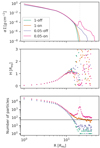 |
Fig. 1. Comparison of averaged surface density and disk height between the models detailed in Table 1. First panel shows the density normalized by the viscosity parameter; second panel shows the scale height H, and the last panel the number of particles in a given radial extent. The dashed vertical line represents the position of the secondary, which is the same for all simulations. The horizontal line in the bottom panel marks 50 particles. |
As the particles get closer to the secondary, differences start to show. Particles are accreted (or “killed”) as soon as they reach a sink particle. In models 0.05-off and 0.05-on, where the sink radius of the secondary is the same as the physical size of the star, particles are allowed to move closer to the companion without being removed from the simulation. Thus, there is a less sharp cutoff in the density. A similar, but much less pronounced, effect is seen for model 1-on, where the resolution of the region close to the secondary is increased by particle spitting.
There is a density increase around the location of the secondary in models 0.05-on and 0.05-off, as particles can exist in close proximity to the secondary star. In model 0.05-off, however, the total number of particles in the simulation (as seen in the bottom panel of Fig. 1) prevents this region from being adequately resolved. The use of particle splitting in model 0.05-on circumvent this issue, allowing for a better resolution, showing a much larger accumulation of matter in this region. On the other hand, in model 1-on, there are a sufficient number of particles at large radii, but the substantial size of the secondary’s sink effectively prevents matter from being captured in its gravitational well. Consequently, only model 0.05-on, which incorporates all modifications to the code, enables the resolution of the structure around the secondary. This is a significant finding that will be thoroughly explored in this paper.
The middle panel of Fig. 1 shows the disk scale height, H. It was calculated by fitting a Gaussian to the volume density ρ(r, z) along the vertical direction for 1 Req slices along r. As expected, the models all behave identically in the inner disk, again assuring that model not unduly disrupted by the modifications. Model 0.05-on has the highest resolution of all models, given the particle splitting, which allowed its height to be measured with greater confidence up to 30 Req, a region which did not exist, for all intents and purposes, in the previous works in Be literature with this SPH code. As shown in the bottom panel of Fig. 1, models without particle splitting have fewer than 50 particles in the radial bands after about 12 Req, making the disk structure unresolved and the scale height and density determination completely unreliable.
In conclusion, our tests confirm that the new features integrated into the code do not hinder us from obtaining results consistent with those of the old code for areas where no differences between them were anticipated. Additionally, we demonstrate that we are now capable of investigating previously obscured structures of the system, including the area around the companion and beyond. Table 2 offers an overview of our upgrades to the code used in this work.
Overview of the upgrades to the SPH code.
3. Models
Using the updated SPH code, we ran a series of simulations with a focus on the previously unresolved regions of the system. As most Be stars in binaries are early-type Be stars, we based this set of models on the well-known Be binary system π Aqr (B1III-IVe). This system was also believed to host more massive companion than usual for Be binaries, consequently leading to stronger effects on the disk dynamics, which is our object of study. We use the values determined by Bjorkman et al. (2002) for the parameters of the Be star and keep the radius of the secondary fixed at 1 R⊙. The fixed parameters in our simulations are shown in Table 3.
Fixed parameters of the SPH simulations.
Our full set of simulations is comprised of 11 models, where the modifications to the code (Sect. 2.2) are always on, and only the orbital period, the mass of the secondary (i.e., the mass ratio q)2, and the viscosity parameter α are allowed to vary (as described in Table 4). For example, model 30-0.1-0.16 has a period of 30 days and α = 0.1 and M2 = 2.06 M⊙ (the mass ratio q = 0.16). Models 30-0.5-0.16 and 30-1.0-0.16 have the same period and M2, but with α = 0.5 and 1.0, respectively. The models designated by 50 and 84 are similar to the three just described, but with different orbital periods. We note that π Aqr’s orbital period is 84.1 days. Finally, models 30-1.0-0.33 and 30-1.0-0.50 are the same as model 30-1.0-0.16, but with a different secondary mass (4.30 M⊙ for q = 0.33 and 6.45 M⊙ for q = 0.5). The companion masses were chosen to represent the higher mass end of stripped stars and He stars, the likely results of a previous mass transfer phase with the Be star, and including MS stars as well. Using more massive companions also maximizes its gravitational effects on the Be disk, aiding our characterization of the dynamics of these systems.
Free parameters for the complete set of SPH simulations.
In the simulations presented here the mass injection rate (Ṁij) is kept fixed at the value of 10−8 M⊙ yr−1, which has been shown to produce disk densities in the typical range of Be star disks (Panoglou et al. 2016; Vieira et al. 2017). Although this choice is physically motivated, it is should be noted that the mass of the gas particles is in truth an arbitrary value, since the disk is not self-gravitating. Therefore, the masses scale with the number of particles and on their status as children of split particles. Most of the particles fall back into the central star due to the natural loss of angular momentum caused by interactions with the matter already in orbit and only about 0.1% of the particles manage to maintain orbit and thus are responsible for building the disk up.
The disk is isothermal in our simulations, with an electron temperature fixed at 60% of the effective temperature of the Be star (Carciofi & Bjorkman 2006). As shown in Sect. 2, the density of a Be disk in the steady-state VDD formulation falls off with radius as ρ ∝ r−3.5 for a thin, isothermal disk. However, the temperature structure of real Be disks is decidedly not isothermal. Carciofi & Bjorkman (2006, 2008), and more recently Suffak et al. (2023) used the 3D nonlocal thermodynamic equilibrium (NLTE) Monte Carlo radiation transfer code HDUST to simulate the temperature structure of a VDD with a fixed density structure and a single star as the radiation source. They find that the temperature at the mid plane is high close to the Be star, but drops for larger radii, before coming up again and reaching a plateau (see, e.g., Fig. 3 of Carciofi & Bjorkman 2008). This property of the disk affects its structure: the decrease in temperature in the mid plane leads to a decrease in the scale height H (Eq. (2), see also Carciofi & Bjorkman 2008), which in turn increases the density in this region and decreases in the density of the upper layers.
It is therefore quite clear that non-isothermal effects influence the disk structure of Be stars and their observables. For the discussion presented here we assume isothermality for simplification. Developing a non-isothermal version of the SPH code is feasible, such as by integrating SPH with HDUST, but it constitutes a substantial undertaking that falls beyond the scope of this paper.
3.1. Overview of the system
The most significant aspect of our modifications to the code is that the resolution in the outer disk is much improved when compared to previous works (Sect. 2.3). Structures that were previously absent can now be seen clearly in the simulations, as shown in Fig. 2. In previous works with this SPH code, only the region inside 20 Req in Fig. 2 was explored, while our simulations cover a region 4 times larger. Thus, we define five distinct regions of interest and analyze them separately, as sketched in Fig. 3: the inner Be disk, the spiral dominated disk, the bridge, the circumsecondary region, and the circumbinary region.
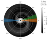 |
Fig. 2. Surface density map of simulation 0.05-on. The overall density structure is qualitatively similar for all simulations calculated for this work, as sketched in Fig. 3. The black circle denotes the Be star, and the black star, the companion. The white circles and numbers mark the radial distance in Req. The three colored bands correspond to the main regions of interest: the wedge that contains the secondary (yellow), the wedge opposite to the secondary (blue), and a wedge that includes the bridge (green). |
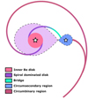 |
Fig. 3. Sketch view of the main regions of the binary Be system. The five main regions are the inner Be disk (pink), the spiral dominated disk (purple), the bridge (teal), the circumsecondary region (blue) and the circumbinary region (mauve). The main characteristics of each region are detailed in the text. |
The inner Be disk is the region least perturbed by the secondary and typically spans a handful of stellar radii in extent. The spiral dominated disk comprises the region from the edge of the inner Be disk to the region that previous studies refer to as the “truncation radius”. In actuality, our simulations show that calling it a truncation is misleading, since it refers in fact to a dynamically complex region that stretches for several stellar radii; Suffak et al. (2022) uses the more appropriate term transition radius. The denser, leading arm extends into the RL of the companion, dumping matter from the Be disk into it. We call this the bridge, as it connects the Be disk to the secondary. Matter accumulates around the secondary forming what we name circumsecondary region. Some of the particles that form this region will be accreted, but part will have enough energy to exit the RL behind the companion. These escaping particles meet up with the other spiral arm, forming one big spiral that envelops the entire system, which we call circumbinary region. Neither the circumsecondary or circumbinary regions were present in any of the previous works that used this SPH code. Each of these regions is explored in the following sections.
Since our simulations have a steady mass injection, once the disk is fully formed and the accretion onto the secondary also stabilizes, the whole system reaches a regime of quasi steady state (Panoglou et al. 2016). This means that between subsequent time steps there is no change in the physical quantities other than that created by the SPH noise and, of course, the rotation of the system. Thus, if the rotation of these steady-state time steps is frozen, namely, if we fix the two stars along the x − y axis of the co-rotating system, the particles present in each of these time steps can be combined into one single “stacked” time step. Since our main focus is on the structures formed after the steady state is reached, this method allows us to artificially increase the resolution of the whole simulation.
As Fig. 2 shows, the system is not axissymmetric, changing considerably in shape and density along different azimuthal directions. In order to quantify and characterize the different regions of the system, we choose to explore its physical quantities (e.g., velocity, density, etc.) along wedge-shaped regions of interest fixed at certain azimuthal angles. Within a given wedge, we compute the quantities at different radial distances and heights (i.e., distance above the equatorial plane). The average quantities are defined as the mass-weighted mean value in a cell, which allows us to account for the different masses of the particles and ignore empty cells in the grid. For the purposes of this work, certain azimuthal directions (given by the angle ϕ in Fig. 2) have more distinct features and are more interesting to be highlighted. These are the direction of the secondary, by definition ϕ = 0 (in yellow), the direction opposite to the secondary, ϕ = 180° (in blue) and the direction containing the bridge between the Be disk and the companion, ϕ = 20° (in green). Figure 2 highlights these three wedges of interest.
3.2. Inner Be disk
In the SPH simulation, mass is lost by the star through the equator at an equal rate in all azimuthal directions. Therefore, one expects that the disk should maintain an axisymmetric configuration near the star and display the signs of the secondary’s action only at greater distances. This is exactly what is observed in Fig. 4, that compares the radial velocities within the first 12 stellar radii of the disk (as per the zoomed in view in this figure compared with Fig. 2). The figure contrasts models 30-0.1-0.16 and 30-1.0-0.16 and confirms that within roughly 3 stellar radii, model 30-0.1-0.16 has a nearly circular configuration. This is also observed in the surface density and azimuthal velocity. We call this region the inner Be disk (pink region in Fig. 3).
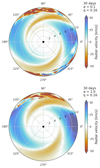 |
Fig. 4. Radial velocity maps for models 30-0.1-0.16 and 30-1.0-0.16. The black dot in the center represents the central Be star. The double spiral structure formed by the elongation of the orbits of the particles is visible in both maps. The over-density occurs in the apastron of the orbits of the particles, where the particles slow down. |
To make a quantitative assessment of the size of the inner disk, we define that the transition to the spiral dominated disk (see the purple region in Fig. 3 and Sect. 3.3) happens when the azimuthal density variation caused by the presence of the companion exceeds 5%. Since the density waves are caused by the changes in the orbits of the disk particles due to tidal interaction with the companion, this shift can be seen in the radial velocity maps of the disk. Figure 4 shows that the spiral waves are noticeable already at about 4 Req for the lower α simulation, while they only become relevant at around 6 Req for higher α.
The inner disk sizes for all models are listed in Table 4, and clearly depend on the period and viscosity more significantly than on the mass ratio, although its effect is not completely negligible. Given the orbital period and the stellar masses, the separation of the two stars is
![Mathematical equation: $$ \begin{aligned} a = \left[\frac{G (M_{1} + M_{2}) P^2}{4 \pi ^2}\right]^{1/3}. \end{aligned} $$](/articles/aa/full_html/2025/06/aa52724-24/aa52724-24-eq18.gif) (18)
(18)
It follows that for larger periods, where the binary separation (a) is larger, the larger the size of the inner disk. This can be seen comparing models with different periods, such as, for instance, 30-1.0-0.16, 50-1.0-0.16 and 84-1.0-0.16. Increasing the viscosity also leads to a larger inner disk, as a more viscous disk grows faster and is more resilient against the tidal torque exerted by the companion. Quantitatively, we can say that for α = 0.1, the size of the inner disk approximately is 20% of the binary separation a; for α = 0.5, it is closer to 28%, and for α = 1.0, around 30%. The effect of the mass ratio is seen when we consider that a also depends on the mass of the two stars: the size of the inner disk is the same between models 30-1.0-0.33 and 30-1.0-050, as the gravitational effects of the companion are also stronger, balancing out the larger binary separation.
In the inner disk, the dominant forces acting on a gas particle are the gravity of the Be star and the viscous force. Even so, the effects of the companion in this region are not completely negligible. The tidal torque removes part of the angular momentum (AM) of the gas, leading to an accumulation of matter (this is the aforementioned accumulation effect of Panoglou et al. 2016). The net result is a decrease in the surface density radial exponent from the canonical steady-state VDD value of m = 2 (Eq. 3). The extent of this change in m is very model dependent, as seen in Table 4, where we estimated the value of m for each model by fitting a power-law to the azimuthal mean of the surface density of the inner disk. The role of each parameter in shaping m is explored below.
Figure 5 compares the surface density, radial velocity, azimuthal velocity, eccentricity of the particles’ orbits, and scale height for several of our models. The accumulation effect is clear when we compare models 30-0.1-0.16 and 30-1.0-0.16, in the top-left panel of Fig. 5. Model 30-1.0-0.16 follows a density drop-off (Eq. (3)) with m ≃ 2.0, as expected from an isolated Be star. Model 30-0.1-0.16, on the other hand, has a much denser inner disk, in addition to being radially smaller (3.7 ± 0.2 Req, m = 0.89). For the same α and q, the larger the inner disk, the smaller the accumulation of matter, thus larger the value for m. Larger mass ratios, such as for models 30-1.0-0.33 and 30-1.0-0.50 lead to larger a, but comparatively smaller m (compared to model 30-1.0-0.16). The disk viscosity also has a significant impact on the accumulation effect. The models indicate that increasing α consistently raises m (i.e., reduces the accumulation effect), which also agrees with previous determinations of m by Cyr et al. (2017). This is simply a consequence of the balance between the viscous torque and the tidal torque of the secondary in this region: the more viscous disks are less subject to the tidal effects of the companion.
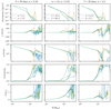 |
Fig. 5. Surface density, radial velocity, azimuthal velocity, eccentricity of the particles’ orbits, and scale height varying with radius for models 30-1.0-0.16 and 30-0.1-0.16 in the leftmost panels, 30-1.0-0.16 and 84-1.0-0.16 for the middle panels, and 30-1.0-0.33 and 30-1.0-0.50 for the rightmost panels. The colors of the lines indicate the wedges along which the quantities are calculated, following Fig. 2: yellow is the wedge pointing to the secondary, blue is the wedge in the opposite direction, and green includes part of the stronger spiral arm. The dotted gray lines show the position of the secondary for the models compared in each column. |
Nevertheless, the inner Be disk is a stable region when compared to the rest of the system. The radial and azimuthal velocities (vr and vϕ) of the particles follow the expected for a quasi-Keplerian motion: vr increases only slowly and monotonically while vϕ follows a power-law with r−0.5, and the eccentricities of the orbits of the particles are also very low for all models. The scale height of the disk also remains remarkably consistent in this region, only deviating in the regime of the spiral dominated disk.
Confirming Be stars as binaries is not straightforward. The standard method for binary detection is spectroscopy, where the radial velocity shifts of the spectral lines can trace orbital motion. In most (all?) cases, Be stars are not found in systems with Main Sequence companions, but rather with evolved stars (Bodensteiner et al. 2020 found no early-type Be+MS binaries in their sample of 287 Galactic Be stars). Thus, as the Be star is the more massive and luminous component of the system, the combined spectra is heavily dominated by the rotationally broadened Be star lines and emission lines from the Be disk, making radial velocity measurements in the visible a challenge. Therefore we look for signs of Be disk disruption in observational data that can point towards hidden close objects. Here we explore which observational characteristics of the inner Be disk may indicate binarity.
The inner Be disk, excluding the Be star itself, is the densest region of the system. It may dominate emission in the short wavelength continuum (from the visible up to the near-infrared), and frequently does so for longer wavelengths. The disk is also responsible for most of the polarized flux (Carciofi 2011). As described in the previous section, the main effect of the companion in this region is the accumulation effect, which causes the slope of the density in the inner disk to be shallower from the standard VDD steady-state prediction (m < 2). Thus, compared to a disk of an isolated Be star, we expect a general increase in V-band emission and polarization fraction, as well as in the emission of lines that form close to the star, such as the He and Fe lines, for systems seen at small and intermediate inclinations. These effects should not be visible in edge-on systems.
To quantify the effects of this change of m on the spectral energy distribution (SED) of a Be system, one can use the pseudo-photosphere model of Vieira et al. (2015). The authors find that the spectral slope of the SED in the infrared regime depends strongly on m, more so than on the base density of the disk. When comparing their models to data in Vieira et al. (2017), the authors find that their results could indicate m < 2 for several targets that were not confirmed binaries. This is a trend in recent works of spectral fitting of Be stars3: Klement et al. (2015) and Rubio et al. (2023) found m = 1.63 and m = 1.33 ± 0.04, respectively, for β CMi, a proposed Be binary4; Klement et al. (2019) find the same for their sample of Be stars consisting in known binaries and (assumed) single Be’s (see their table 7); de Almeida et al. (2020) finds m = 1.5 for o Aqr; and Marr et al. (2021) finds m = 1.1 for 66 Oph.
The changes in the spectral slope of the SED of Be stars might be signs of binarity, but might also be due to other factors, such as thermal effects not considered in the derivation of the steady-state VDD approximation, radially variable viscosity, and duty cycle of the Be activity (Vieira et al. 2017). However, the other regions of a Be binary system also have expected observational effects that could in combination point to binarity more unambiguously. This is explored in the following subsections.
3.3. Spiral-dominated disk
In a quasi-Keplerian disk, as an isolated Be disk should be in theory, the radial velocity should be low, much lower than the sound speed (Bjorkman & Carciofi 2005), increasing slowly with radius, but showing no azimuthal dependence. Our simulations of binary Be stars, along with previous works, indicate that in these systems the orbits of the individual particles can be highly perturbed by the secondary’s potential. A direct consequence of these changes in the velocity field of the particles is the excitation of two-armed density waves, as seen in Fig. 4.
In this m = 2 mode, the motion of the particles can be well described by epicycles along their orbit around the Be star, with an epicentric frequency that is twice the orbital frequency, similarly to the motions of stars the disks of galaxies (Binney & Tremaine 2008, Chapter 3). Thus, there are two apastrons and two periastrons in the orbits of the particles. Thus, the eccentricity measured in Fig. 5 (forth row) is instantaneous average of the eccentricity in the wedge. The spiral structure, a consequence of this orbital motion, consists of one arm that leads the companion and another, less dense arm that trails 180° behind. The consequences for vr and vϕ are shown in the second and third rows of Fig. 5, and are present in all models, with the extreme values for both vr and vϕ happening between the two apastrons and periastrons of the orbit. In the azimuthal direction that includes the stronger density arm (green wedge defined in Fig. 2), the general behavior of the surface density is of a decrease (much faster than the inner disk), followed by a bump (the arm itself), and finally a more dramatic falloff. The first decrease has counterparts in the direction of the secondary (yellow wedge) and its opposite direction (blue wedge), and could also be seen in the works of Okazaki et al. (2002) and Panoglou et al. (2016). However, given the resolution of their simulations, the second decrease was sharper and more definitive: it represented a true truncation of the disk. With our updated simulations, we see that what was called the truncation radius is really a region spanning several stellar radii where the density of the disk decreases, but at azimuthally variable rates. Along the green wedge, the density increases again when the stronger density arm (that will become the bridge – see Sect. 3.4) crosses it; in the yellow band, the increase happens in the position of the secondary (marked by the dotted vertical lines in the plot); and in the blue band, the increase is much fainter (for some models, such as 30-1.0-0.33 and 30-1.0-0.50, imperceptible in the plot), due to the weaker, trailing spiral arm, expanding away from the system. In this region, the disk scale height also begins to deviate from the simple power-law expected from a Be disk, as also seen in Cyr et al. (2017) in their simulations of misaligned Be binaries.
Figure 6, where each line corresponds to the mean value (averaged over radial bins) of the surface density, vr and vϕ for discrete wedges of 0.125 radians each, offers a more complete view of the dependence of the density and velocity fields on radius and azimuthal angle. The outwardly expanding spiral arms are clearly seen in both density and radial velocity.
 |
Fig. 6. Mean surface density, radial and azimuthal velocities for discrete wedges in ϕ of 0.125 radians each (from ϕ = −π to π, where ϕ = 0 is the direction that includes both the Be star and the secondary). The model parameters are indicated at the top of each column. The top and bottom plots compare models with low and high α, respectively. Dashed lines in the middle panel represent resonance radii close to the nodes (see text for details). |
The effects of binarity on the radial velocity field are especially noticeable, as velocities rise much above the few km s−1 expected in quasi-Keplerian decretion disks. They surpass the sound speed in the disk and increase even further going towards the companion and into the bridge (Sect. 3.4). The reason for this difference is that the radial velocity in isolated Be disks depends only on the viscous transport of matter through the disk. Observations and models agree that Be disks are not wind-driven, but grow through viscous torque and are rotationally supported; therefore, the radial velocity field does not change much with radius for an isolated star. When a companion is added, however, its tidal interaction with the Be disk deviates the orbits of the particles, from the circular and coplanar orbits of an isolated Be disk to elliptical, non-coplanar orbits (see, e.g., the fourth panel of Fig. 5). Thus, the significant variations we see in vr in Figs. 5 and 6 are not due to changes in the rate and velocity of matter ejected from the Be star into the disk, but rather to orbital disturbances caused by the companion.
As with the inner disk, the size and behavior of the spiral dominated disk scales with the period of the system. The tightness and “strength” of the spirals (the range of their deviation in density, as expressed in Eq. (3), and the velocity from the standard Be disk solution) are, on the other hand, more sensitive to the viscosity. The emergence of the spiral arms can be seen in the surface density and vr plots in Fig. 6, particularly for the low α models. The radial velocity exhibits a nodular pattern with points of near-zero velocity aligning with various resonance radii of the orbit. For model 30-0.1-0.16, the resonance radii closer to the visible nodes are 6:1, 9:1, 12:1, and 16:1. For model 50-0.1-0.16, they are 6:1, 10:1, 14:1, and for model 84-0.1-0.16, 7:1 and 11:1. No definite and clear pattern were detected, neither a correlation with the model parameters. For our high α models (bottom panels of Fig. 6), only one node is clearly identifiable. The closest resonance radii are 7:1, 8:1 and 9:1 for models 30-1.0-0.16, 50-1.0-0.16, and 84-1.0-0.16, respectively.
Figure 7 offers another view of the spiral arms. Each line represents the surface density as a function of ϕ, at different fixed radial distances from the Be star (indicated by the color map). The tightening and strength of the spirals and the overall size of the region are seen more clearly. Models with larger α have much more spread out and weaker arms, as the density variation is lower. The density variation between the leading and trailing arm is also lower. For the same α and different periods, such as for models 30-0.1-0.16 and 84-0.1-0.16, lower periods show tighter and denser spirals.
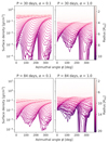 |
Fig. 7. Surface density as a function of ϕ, at different fixed radial distances from the Be star (shown by the colormap), for models 30-0.1-0.16 and 30-1.0-0.16 (top), and 84-0.1-0.16 and 84-1.0-0.16 (bottom). |
To describe the shape of the density waves, we analyzed the surface density curves of Fig. 7, fitting the azimuthal position of the two peaks with an exponential function
 (19)
(19)
where A and B are free parameters related to the orbital phase and density of the region, and γ is a parameter that measures how tightly wound the spirals are (Cyr et al. 2020). The winding parameter γ for each model (and for each spiral arm) are presented in Table 4. We find that γ consistently decreases with viscosity, as the overall increase in radial velocity in the disk leads to less eccentric particle orbits, and (more weakly) with the period of the system. Increasing mass ratio also leads to tighter spirals. For all models, the spiral arm that leads the secondary is marginally less wound than the trailing arm. This can be also seen examining Fig. 7. Our results agree with Cyr et al. (2020) for their coplanar models (see their Tables 2 and 3).
The clearest observational counterpart of two armed density waves are the violet/red (V/R) variations in double peaked emission lines, in particular Hα. These variations are caused by the cyclic increase and decrease in density in either side of the disk as the system rotates and the density waves move from side to side. While the m = 2 mode itself is not asymmetric, the two arms are unequal in strength and winding. Furthermore, the optical depth attenuation of the arms depend on the orbit, due to disk flaring; i.e, the arm currently further from the observer will be more affected. For Be binaries such as π Aqr (Zharikov et al. 2013), γ Cas, 60 Cyg and HD 55606 (Chojnowski et al. 2018), they phase very closely to the period of the system, but that is not always the case. Recently, several examples of orbital phase-locked V/R variability have been found and measured by Miroshnichenko et al. (2023). Furthermore, they found that the amplitude of maximum V/R value decreases with increasing orbital period (see their Fig. 18). A quantitative estimate from our models show that there is anti-correlation between the binary separation and the amplitude of the density variation in the spiral dominated disk, which likely translates observationaly as the V/R amplitude-period relation detected by Miroshnichenko et al. (2023).
One-armed density waves are also excited in Be disks with no relation to their binarity (Okazaki 1991), leading to V/R variations with much larger amplitudes and generally much longer periods (typically longer than a few years as the period is set by the precession the of the one-armed wave around the star, e.g., ζ Tau, Carciofi et al. 2009). The m = 1 waves, therefore, give rise to phenomena similar to those of the m = 2 waves, but can be easily differentiated by their longer periods and larger amplitudes.
How tight and how strong the spiral arms are will influence its effects on the observables, which also depend on the inclination angle of the system. Larger V/R variations will happen when there is stronger left-right asymmetry in the disk with respect to the observer. More spread out waves will produce larger V/R variations, while this asymmetry will clearly be smaller (washed-out) for more tightly wound spirals, as they decrease the density and velocity contrast in the emitting area of the disk.
Panoglou et al. (2018) studied the expected behavior of Hα line profiles by calculating radiative transfer simulations for systems of coplanar, circular Be binaries, based on the SPH simulations presented in Panoglou et al. (2016). Their models agree with our expectations for the general behavior of the V/R variations caused by the density waves, but we note that their radiative transfer calculations are based only on the density structure of the perturbed Be disk given by their SPH simulations: their models do not consider the velocity field of the particles, and include only what we refer to as the inner Be disk and the spiral dominated disk, fully truncated by the companion. Thus, any observational effects of the bridge, circumsecondary region, and circumbinary outflow, and the relevant effects of the velocity profiles of the particles, are not considered in their Hα calculations.
Effects in the polarization are also expected to arise from the disk perturbations. Variation in the position angle (PA) of ζ Tau with phase due to m = 1 density waves is well established (Schaefer et al. 2010). Similar effects have been predicted to exist in the case of m = 2 waves of Be binaries by (Panoglou et al. 2019). However, the observational detection of this phenomenon remains to be achieved.
An effect that should also be seen in binary Be stars is variations in the position of the central reversal in double peaked lines, in particular for shell lines. Shell line profiles are characterized by unusually deep central reversals, caused by absorption of stellar light by the disk, and appear in Be stars observed at high inclination angles (closer to edge-on). In symmetric disks, with small radial velocities the shell profile is symmetric, narrow and centered at the systemic velocity of the star. For disks with asymmetries such as the ones discussed here, the projected velocity along the line of sight can be rather large, as shown in Fig. 8 for model 84-0.5-0.16 and observes at two different positions (ϕ = 18° – right, and 350° – left), indicated as the dashed lines. The regions corresponding to different projected velocities are marked in different colors. The light emitted by the star travels through regions with quite different radial velocities before reaching the observer, in stark contrast to a symmetric disk model. Therefore, it is expected that the shell absorption will not necessary be centered at the systemic velocity, and will likely be broader due to the larger range of radial velocities. This effect was observed in the Be+sdO binary HD 55606, which goes through orbital phase dependent intermittent shell phases. Chojnowski et al. (2018) shows that the wings of the Hβ, Hγ and Hϵ lines of this system do not shift with phase, while the shell feature does (see their Fig. 7). This central reversal variation has been little explored in the literature and offers great diagnostic potential in characterizing the properties of binary Be stars.
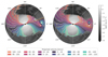 |
Fig. 8. Projected velocities along the line of sight of an observer at ϕ = 18° (left) and ϕ = 350° (right), for model 84-0.5-0.16. The background black and white map show the surface density of the system. The various colored bands map out the projected velocities, while the dashed orange lines indicate the direction of the observer. The black circle denotes the Be star, and the black star, the companion. |
3.4. Bridge
Along with the accumulation effect and the spiral arms, the truncation of the Be disk is a known effect of binarity. As the disk grows, the resonant torque of the companion takes its angular momentum, effectively impeding its further growth. In the SPH simulations of Okazaki et al. (2002) and Panoglou et al. (2016), this truncation happens at around the 4:1 to 5:1 resonance radii and is rather sharp, given their larger size of the secondary’s sink (already discussed in Sect. 2.3). Our updated simulations show a different perspective: the disk is not totally truncated, but is elongated along the Roche potentials of the binary system. The disk scale height in this truncation region, shown in the bottom panels of Fig. 5, behaves very differently depending on the azimuthal angle: the decrease is sharp for the ϕ = 0 wedge (that contains the secondary) but is not present in the opposite direction (ϕ = 180° wedge), except for a subtle decrease in models 30-1.0-0.33 and 30-1.0-0.50. Note, however, that, given the low resolution of the system towards ϕ = 180°, it is difficult to fully characterize the scale height in this direction.
Our models show that matter flows from the Be disk via two exit points, one towards the companion and another opposite to it. These exit points are located around the L1 and L3 Lagrangian points (see Fig. 9), but, given the rotation of the system, they are leading L1 and L3 in the direction of rotation. The surface density maps of Fig. 9 for models 30-1.0-0.16, 30-1.0-0.33 and 30-1.0-0.50 show that the mass ratio of the system not only affects the overall size of the Be disk, but also the efficiency of mass leakage through L3. The same effect can be seen in the bottom right panel of Fig. 5, where the scale height of the disk decreases more or less equally in all directions for models 30-1.0-0.33 and 30-1.0-0.50, suggesting a more evenly truncated disk than seen for model 30-1.0-0.16.
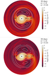 |
Fig. 9. Density maps for models 30-1.0-0.16 and 30-1.0-0.33, showing the Roche equipotential contours and the Lagrangian points. The black circle marks the Be star, and the black star, the companion. |
The transfer of matter from the Be disk into the Roche lobe of the companion happens through the bridge, an extension of the leading spiral arm that connects the two (light green region in Fig. 3). Most of the mass that leaves the disk of the Be star does so through the bridge, which is by far the densest region at this radius (for instance, in model 30-1.0-0.16 the bridge is seen as the density peak at about 12 Req, green line in the top right panel of Fig. 5). It is also the region with higher values of radial velocity compared to the rest of the Be disk, as the material is accelerated towards the companion and then enters its RL close to the L1 point. Its counterpart, the trailing arm opposite to the companion, is the second point of mass loss for the Be disk, near L3. This arm grows outwards undisturbed, eventually merging with the stream that forms the circumbinary region (Sect. 3.5).
Figure 10 shows a zoomed-in 2D map of the bridge for model 30-1.0-0.16, with the color indicating the radial velocity of the gas (in the reference frame of the primary). Since the radial velocity of the secondary is zero (due to its circular orbit), the plot illustrates the significant velocity differences between the secondary and the surrounding gas as material accelerates along the bridge towards the companion. The positions of the two density arms are marked by the xs in the plot. Superimposed on the image are contour lines indicating the azimuthal velocity. These lines reveal that the Be disk is now far from Keplerian, even exhibiting negative azimuthal velocities, indicating retrograde motion.
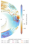 |
Fig. 10. Map of radial (in full colors) and azimuthal (contours) velocity for simulation 30-1.0-0.16. The gray xs mark the regions of highest density for that given radii, tracking the two spiral arms. The black half circle marks the Be star, and the black star denotes the companion. |
Observationally, the steep density fall-off of the truncation region is seen as a steepening of the slope of the spectral energy distribution (SED) in long wavelengths, around the centimeter/millimeter regions. This effect is referred to as the SED turndown (Waters et al. 1991; Klement et al. 2017). SED turndowns have been detected in several Be stars in Klement et al. (2019), both in confirmed binaries (e.g., γ Cas) and in (at the time) presumed isolated stars (e.g., β CMi). As previously discussed, confirming binarity in Be stars is a complex task due to the brightness ratio between the Be and its usually evolved companion, and to the effects of stellar rotation and of the disk on their spectral lines. The detection of the SED turndown, while an indicator of disk truncation, does not automatically mean a companion is present, as other causes for truncation have not been discarded (see, for instance, the results of Curé et al. 2022 for the transonic disk solution, and Kee et al. 2016 for radiative ablation of the disk). Our models show that in reality it is more complex: the extent of the truncation region varies with azimuth due to the disk’s elongation. Additionally, the bridge acts as a funnel through which most of the disk mass flows, complicating matters by extending a small part of the disk to larger radii.
Peters et al. (2016) provides a prime example to understand the impact of the bridge on the observations. They assumed a “circumbinary disk” model to explain the shell absorption features in Si II and III and S III lines of HR 2142, a known Be+sdO binary. Their model is close to what is shown by our simulations: a disk truncated by the companion, but where material travels through the L1 point towards the companion in streams (similar to what we call the bridge in this work). The opacity of the stream would be responsible for the shell absorption as the stream passes in front of the Be star. Peters et al. (2016) also predicted the leak of material through L3, and the formation of a circumbinary disk, in agreement with our models.
In Peters et al. (2016)’s observations of HR 2142, the shell features occur in two phases. In the what they called the primary phase (when the observer is at around ϕ = 18°), the absorption features span a velocity range of +10 to +160 km s−1; in the secondary phase (observer around ϕ = 349°), velocity ranges from −40 to +20 km s−1. To investigate whether these phases are compatible with what we expect from the bridge in our simulations, we show in Fig. 8 the projected velocities for observers at ϕ = 350.0 and ϕ = 18.0 (with the bridge in front of the Be star) for model 84-0.5-0.16. As the figures show, there is indeed material in the bridge and circumsecondary region (see Sect. 3.5) with radial velocities roughly matching the ranges seen by Peters et al. (2016). Other disturbances on line profiles due to the bridge can also appear. Whether this contribution is in emission or absorption depends on the inclination angle of the observer: absorption features are expected for near edge-on orientation and vice-versa. Here the nature of the companion becomes important, as this region is close enough to be irradiated by it. If the companion is a hot subdwarf, as is the case for many Be stars, including HR 2142, it is possible that the bridge will be further heated up by the secondary, changing the emission/absorption line strengths. Traveling features (in absorption or emission) can, therefore, be caused by the bridge, and might be indicators of binarity.
3.5. Circumsecondary region
Via the bridge, material from the Be disk enters the RL of the secondary. Given the boundary conditions previously set in the SPH code of Okazaki et al. (2002), no structure of any kind could be seen around the secondary in their Be binary simulations. Hayasaki & Okazaki (2004) bypassed this issue by running a simulation focused only on the accretion stream (the bridge). The boundary conditions for this simulation were chosen based on the parameters of the particles that were accreted by the companion (i.e., entered its RL) in one of the simulations of Okazaki et al. (2002) (based on a coplanar BeXRB system with e = 0.34). Their results show that a Keplerian disk is formed around the companion for all their simulations, which explored different equations of state and viscosity parameters. Martin et al. (2014), using SPH simulations with the code PHANTOM (Price et al. 2018), also shows that an accretion disk is formed. These works investigated tilted and eccentric systems for which there is an extended period of time where no new matter and AM enters the RL of the companion. During this time, the matter already inside the RL, dumped there in the previous encounter with the Be disk, can reorganize itself and form a disk from which the companion accretes. We note that these works keep the artificial SPH viscosity (αSPH) fixed and do not considered the effect of the secondary on the scale height of the disk, which lead to increasing Shakura-Sunyaev α in the vicinity of the companion (with the exception of Hayasaki & Okazaki (2004): as it considered only the region of the gravitational sphere of the secondary, where the particle distances are measured from the secondary, so no artificial increase in α has occurred). Our simulations use a prescription for the viscosity of Be disks in binary systems where the SS α does not vary in time or with radius (see Sect. 2.2.3).
In our simulations, from the moment the Be disk reaches a quasi steady-state configuration (see Sect. 4), there is a constant injection of mass and AM into the RL of the companion. The velocity and density of this particle stream, as discussed in Sect. 3.4, are parameter dependent, and so is the circumsecondary region. The yellow lines in Fig. 5 show the properties of the material in the yellow wedge of Fig. 2, a region that contains the secondary and the majority of its RL. There is a tremendous increase in density in this area, even rivaling the mean density of the spiral dominated regions of the Be disk. The same is also shown in the cross section contour plots of the volume density (considering a height z = −10 to 10 Req) of the circumsecondary region for all models are in Fig. 11 (black lines). The orbital period has the strongest effect on the density of the circumsecondary region: lower periods lead to denser structures. The effect of α is more clearly seen in the velocity profile, where lower viscosity models have a larger rotational velocity, exceeding 20 times the radial velocity, in the whole circumsecondary region. This is likely due to the fact that in large α models the material comes from the bridge with higher radial velocities and has higher viscous torque. For higher mass ratios (bottom rows of Fig. 5), the concentration of matter is larger and so is its rotational velocity, as a more massive companion has a stronger gravitational pull.
We consider the circumsecondary structure (where particles are gravitationally bound to the secondary) to be disk-like (i.e., dominated by rotation, shown in the blue region in Fig. 11) when its orbital velocity is larger than its inflow and outflow radial velocities, in the frame of reference of the secondary. Figure 11 shows the ratio of the azimuthal and radial velocity fields for all models. The deformation of the structure in the higher α models, and their densities are lower when compared to models with α = 0.1. For models with higher mass ratios, the rotational component of the velocity is very significant, even more so than for low viscosity models. Even so, all models show a large portion of their circumsecondary regions to be dominated by rotational velocity, and show circular symmetry in the density. We conclude that the structure can be considered disk-like in all our simulations, keeping in mind that its size and density are highly dependent on the system’s orbit. We note again that our simulations are purely hydrodynamical and isothermal, lacking radiative transfer. Consequently, the actual structure of the circumsecondary region, particularly very close to the companion, cannot be fully determined at this time. Additionally, it may be important to consider the winds of stripped stars in this context.
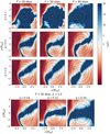 |
Fig. 11. Map of the ratio of vϕ to vr in the reference frame of the secondary, indicated by a black star in the center. Cross section contour plots (at z = 0) of the volume density (log(ρ), in g cm−3, integrated from z = −10 to 10 Req) of the circumsecondary region are shown in black. The Be star is to the left, not shown. |
Particles are continuously accreted by the companion throughout the simulation, as shown in Fig. 12. The dependence of the accretion rate by the companion (Ṁacc) with the evolution of the simulation is due to two main factors: the time necessary for the disk to grow and reach the orbit of the companion, and the size of the structure formed around the companion as matter accumulates inside its RL. The amount of days of constant mass injection needed for Ṁacc to grow above 1.3 × 10⁻¹¹ M⊙/year (an arbitrary definition based on the inflection points of Ṁacc in Fig. 12) scales with period, α, and mass ratio, and can be viewed as a rough estimate of how many binary orbits it takes for the Be disk to build-up completely in each model. These estimates are given in Table 4. As expected, the Be disk build-up time decreases with increasing α (Eq. (21)), but are not consistent across different periods and mass ratios, which might indicate it is due to SPH uncertainty rather than being a physical property. We also emphasize that these estimates are for the growth of Be disks subject to constant mass injection from the Be star, and depend on the mass injection rate, Ṁij. As discussed in Section 3, Ṁij in our simulations is fixed to 10−8 M⊙ yr−1, which also fixes the particle mass in each simulation.
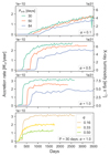 |
Fig. 12. Accretion rates and X-ray luminosities for our models. In the first three panels, different colors indicate period, and q and α remain fixed. In the fourth panel, colors indicate q, and period and α are fixed. |
The most commonly used physical descriptions of mass accretion are the Bondi–Hoyle–Lyttleton (BHL, see Edgar 2004, for a review) flow accretion and Roche lobe overflow (RLOF). BHL considers accretion onto a star from a supersonic, infinite, homogeneous gas cloud, and is mostly used for accretion of winds. RLOF is used in the context of binaries, where one star inflates and fills its Roche lobe, initiating mass transfer. In RLOF, mass flows through the Lagrangian point L1 onto the RL of the companion, and is then accreted. The case of Be binaries exhibits clear similarities to both BHL and RLOF accretion scenarios. As in BHL, matter from the Be disk flows towards the secondary with high radial velocities; and as in RLOF, the disk expands enough to reach the RL limits. As seen above, mass transfer does not happen exactly through the L1 point as a regular RLOF, but ahead of it, due to the non-zero rotational component of the disk at the disk/companion interface, and due to tidal friction between the Be disk and the tide-raising secondary.
The BHL accretion rate is given by
 (20)
(20)
where the impact parameter b is defined as b = 2GM2/vrel2, and ρ and vrel are the relative density and velocity of the flow. In the case of winds, where the BHL prescription is commonly used, these quantities are defined in a region where they are not yet affected by the gravitational pull of the accretor. However, these quantities are not as straightforward to define in the case of a accretion from a Be disk. Even in the case of an isolated Be star, the decretion disk has radially and vertically dependent density and velocity profiles. For a disk perturbed by a companion, these profiles become even more complex (as described in previous sections). Therefore, there is virtually no location in the disk where the presence of the companion is not affecting the flow of the material.
The BHL prescription does not account for the viscous forces acting on the system, and the non-uniform structure of the disk make it difficult to apply it directly to the case at hand. However, we can (crudely) estimate what the BHL accretion rate would be considering the density and velocity structures of an isolated Be disk, if a companion instantaneously appeared in the middle of the disk at a distance from the Be star at a given separation, with no time given for it to alter its density and velocity structures. Assuming a Keplerian disk, the relative velocity vrel between the disk material and the companion in orbit around the Be star will be the radial velocity of the disk at that radius, which are on the order of tens of km s−1. The density will be given by Eq. (4). Considering also that only the material inside the RL can be accreted, even if the impact parameter b is larger (which is the case, given the low relative velocity), we find BHL mass accretion rates on the order of 10−11 M⊙/year, about 20 times smaller than we find in our SPH simulations (∼2 × 10⁻¹⁰ M⊙/year).
The overall shape of the accretion stream in our coplanar Be binaries is nearly identical to wind-RLOF (WRLOF – see Mohamed et al. 2007), where the wind (and not the star itself) is what fills the RL. In WRLOF, accretion rates can exceed wind BHL prediction by ≈100 times, against the 20 times larger estimate we find in our “disk-RLOF”. This discrepancy is caused by the viscous forces acting on the system and the disk rotation. The bridge has an azimuthal velocity lower than Keplerian, as the gravity well of the companion decelerates the material azimuthally, while accelerating it radially. This leads to a larger relative velocity between the bridge material and the companion, making capture and accretion more difficult.
The maximum value of Ṁacc strongly depends on the orbital period and on α. In our models, the Be disk is fed constantly, and the rate of mass flow eventually reaches a steady-state. This steady-state indicates that the amount of matter injected and ejected from the system (leaving either via accretion onto the secondary or to the circumbinary structure), is balanced. Thus, the steady-state accretion rate will be controlled by several factors that set the mass flow rate leaving the Be disk and the fraction of it trapped by the circumstellar structure. All this depends on the model parameters. Similarly, as seen in Fig. 11, the size and density of the circumsecondary region also depend on the viscosity and orbital period, as does the amount of matter exiting from the L3 point. For models with α = 0.5 and 1.0, the maximum value of Ṁacc is mostly dependent on the period, reaching similar values for both viscosity parameters after the system becomes stable. For models with α = 0.1, this value is systematically lower, and so is the difference between different periods. These are the models that, according to our definition, form an accretion disk. The presence of this rotationally supported structure regulates the accretion rate.
A counter-intuitive result is that Ṁacc decreases with increasing q. The same behavior was observed by Franchini et al. (2019) in their simulations of misaligned Be binaries. They tentatively attribute this to the fact that a more massive companion could induce stronger torque in the Be disk, thus leading to a stronger truncation and less material entering the RL of the companion. However, our simulations show that while the Be disk is indeed smaller (Fig. 9), the circumsecondary region is actually larger for higher q, and has a strong rotational velocity (rightmost panels of Fig. 5, bottom maps in Fig. 11). A plausible explanation for their lower Ṁacc is that there is a larger amount of material leaving the system through L2 in these models, as shown in Fig. 9.
The accretion of matter from Be decretion disks by their companions is a well-established phenomenon. BeXRBs, comprised of a Be star with a compact companion (a neutron star or black hole), make up half of the high-mass X-ray binary population in the galaxy. Their X-ray emission is consequence of the material of the Be disk falling onto the companion. There are two types of outbursts in BeXRBs: the weaker, shorter Type I outbursts and the brighter and longer Type II outbursts. Type I outbursts happen when the eccentric orbit binary neutron star accretes material from the Be disk at periastron (Okazaki 2001; Negueruela & Okazaki 2001), while Type II outbursts are less frequent, not periodic (Monageng et al. 2017), and are caused by a large amount of material being suddenly accreted by the companion. This abrupt increase in accretion can be caused by Kozai-Lidov oscillations in the Be disk, excited by a misaligned companion (Martin & Franchini 2019).
The observational consequences of the accretion will be determined by the nature of the companion. If the companion is a sub-dwarf, there is no direct consequence of the accretion itself on the observables apart from, perhaps, very faint and soft X-ray emission (Nazé et al. 2022). If it is a compact object (a neutron star in particular), strong X-ray emission is expected, as evidenced by the dozens of known BeXRBs. The X-ray luminosity can be written as  , with η = 1 (as per Okazaki 2001), and MX and RX the mass and radius of the proposed compact object. The values for models with q = 0.16 are plotted in Fig. 12, and range from 4 to 7.5 × 1031 erg s−1. For model 30-1.0-0.33, LX ≈ 1.0 × 1032 erg s−1, and for model 30-1.0-0.50, LX ≈ 7.7 × 1031 erg s−1, respectively the highest and second highest values in all models. All estimates are much lower than the common values of 1034 − 1035 erg s−1 found for persistent BeXRBs. Considering the mean accretion rates of 2 × 10⁻¹⁰ M⊙/year found in our models, a companion with a radius of RX ≈ 0.005 Req for q = 0.16, or RX ≈ 0.01 Req for q = 0.33 and q = 0.50 would reach an X-ray luminosity of 1034 erg s−1. As these radii estimates are about three times larger than the typical size of a WD, and hundreds of times larger than a typical NS, the mean X-ray luminosity of BeXRBs would be easily reached (and surpassed). Thus, in our estimates, a NS or WD in such an orbital configuration would emit strongly in X-rays. However, our models are coplanar and circular, an unlikely configuration for a BeXRB with a NS since when the NS is formed, the supernova kick could have an impact on the orbit. How significant its impact depends on the previous evolution of the system, the amount of mass ejected during supernova, and the magnitude and direction of the subsequent kick (we point to the ongoing discussion over the formation of BeXRB SGR 0755-2933 in Richardson et al. 2023; Larsen et al. 2024; Richardson & Eldridge 2024). If the kick does indeed disturb the orbit significantly, the system would not have time to circularize and flatten again in the lifetime of the Be star (see Liu et al. 2019, for the discussion over proposed Be+black hole binary LB-1).
Recent X-ray observations of Be+sdO binaries show detection of faint X-rays of the same order of magnitude as our models (Nazé et al. 2022), but the authors noted that they did not find a correlation between the X-ray luminosities and the periods of the systems or the properties of the companions. This result does not exclude that this X-ray emission might be coming from accretion onto the companion, or from disk-wind interactions in its vicinity.
The circumsecondary disk might also be directly studied by observations. As discussed on the observational expectations for the bridge (Sect. 3.4), the companion will irradiate this region, and its consequences will depend on the density and kinematics of the material. Evidence of a material around the secondary was seen in Be binaries π Aqr (Bjorkman et al. 2002) and, more recently, o Pup (Miroshnichenko et al. 2023). A very clear observational example of emission lines from a disk around a companion in a Be binary is HD 55606, a Be+sdO system. Chojnowski et al. (2018) detected strong double peaked He I lines whose radial velocity shifts are consistent with the companion. The double peaked nature of the emission also indicates the material is rotating, thus suggesting a disk around the sdO. Their Fig. 9 shows their schematic view of the system, similar to Peters et al. (2016)’s for HR 2142, but without invoking the mass stream crossing L1. The authors assume the Be disk extends past its RL to explain the O I 8446 Å lines, and attribute the transient shell phases of the Balmer lines, the O I 7771–7775 Å triplet, and occasionally in the Paschen series, Si II, Fe II, and Ni II, to the denser parts of the spiral dominated disk. HD 55606 is a circular and coplanar binary, with a period of 93.76 ± 0.02 days and q = 0.14 ± 0.02, quite similar to our models with Porb = 84 days and q = 0.16. These models (as all our models, in fact) have the same basic structure, shown in Figs. 2 and 9, and simplified in Fig. 3: the Be disk extends past its RL only in certain regions, there is always a bridge connecting Be disk and companion, and there is always a circumsecondary structure. Future works on the complex radiative transfer taking place in our simulations will answer whether the emission in O I 8446 Å and the shell features can also originate from the bridge (as suggested by Peters et al. 2016) or the circumsecondary structure. Additionally, the double peaked, symmetric He I line profiles of HD 55606 are qualitatively supported by our models, that suggest that roughly aximmetric circumsecondary structures are formed (see, e.g., models 84-x-0.16 – last column of Fig. 11).
Another observable that has provided interesting insight into Be binaries is interferometry. The recent work of Klement et al. (2024), for instance, looks at optical/near-IR interferometry from CHARA/MIRC(-X) for 37 Be stars with spectroscopic signs of binarity. HR 2142 was one of their targets, for which they also had VLTI/GRAVITY spectrointerferometry for the Brγ line. The standard geometric model used in interferometry to describe Be stars and their disks consists of a uniform disk representing the Be star, a 2D Gaussian for continuum disk emission and a Keplerian rotating disk for line emission. For Be binaries, another uniform disk is added to represent the companion. A companion introduces distortions and asymmetries in the disk, which are seen in the interferometric observables, mainly the visibility and the closure phase. The visibility is sensitive to the geometrical size of the source in the sky, while the closure phase is more sensitive to asymmetries in the emission. In order to reproduce the GRAVITY data of HR 2142, an unresolved emission line component had to be added to the model, which their best fit placed in the vicinity of the sdO companion, thus confirming the presence of circumsecondary material.
Future studies are planned to investigate the interferometric signals of the models presented in this paper, and how these signals could be used to detect new Be binaries through interferometry or to characterize the circumstellar properties of known ones. There are currently several interferometric instruments in operation that combined would provide a very complete overview of the structure and dynamics of the Be disk: CHARA/SPICA (covering the visible band, including Hα, Mourard et al. 2017), CHARA/MIRC-X (near-infrared bands J and H, Anugu et al. 2020), VLTI/GRAVITY (near-infrared K band, including Brγ, GRAVITY Collaboration 2017), and VLTI/MATISSE (mid-infrared L, M and N bands, including Brα, Lopez et al. 2022). CHARA/MIRC-X has already been used to confirm several binaries, and VLTI/GRAVITY have already proved its capability in detecting signals from the circumsecondary disk. CHARA/SPICA could conceivably detect the spiral structure in the Be disk in addition to material around secondary, both of which should have big impacts on Hα. Finally, in the near future, the upgraded GRAVITY+ will be able to observe fainter Be stars with higher spectral resolution, greatly increasing our sample size of observable Be binaries.
3.6. Circumbinary disk
Circumbinary disks around multiple systems are important and active agents in star and planet formation, in mass transferring systems, and in post-asymptotic giant branch binary systems (Kluska et al. 2022). In the particular case of binary Be stars, the material of this circumbinary disk comes from the Be disk, not from winds or envelope ejection. The possibility of circumbinary disks in Be binaries was first suggested by Peters et al. (2016) for HR 2142, based on the gaps that protoplanets form in protoplanetary disks. The SPH simulations of BeXRBs of Franchini et al. (2019) show the formation of this type of structure around their misaligned, eccentric systems, which suffer from strong Kozai-Lidov oscillations. The recent work of Martin et al. (2024) explores the dependence of the Be disk size with the disk scale height, and also shows the formation of a circumbinary structures. However, our work is the first to fully explore the region beyond the “truncation” of the Be disk and its observational consequences with detail.
As shown in Fig. 2, the circumbinary disk is formed from matter that escapes from the companion through the L2 point, and matter that escapes the Be gravitational well through L3 (as the system is rotating, the exit points are not exactly at L2 and L3, but around them). While L2 is a exit point for all simulations, L3 can be “clogged” by the resonant torque of the companion when q increases: already at q = 0.33 there is virtually no mass loss from L3 in our Porb = 30 days model, as shown in Fig. 9. The material in the circumbinary disk has rotational and radial velocities on the order of hundreds of km s−1, but is bound gravitationally to the system in the radial extent we considered in our simulations. Given more time to evolve and grow, with the constant injection of matter and AM coming from the Be star, the circumbinary disk could be sufficiently extended to escape the system.
Though much less dense than the Be disk, the bridge, and the circumsecondary structure, the circumbinary disk has non-negligible density and may have observational counterparts. In Klement et al. (2017, 2019), the authors find that many Be stars have an SED turndown, an effect caused by disk truncation. However, for many Be stars, the shape of the SEDs is inconsistent with a true truncation of the disk by a companion. The slope of the SED after this truncation radius indicates that there is some material beyond the orbit of the companion emitting in IR and radio. The authors find this evidence of a circumbinary disk for all their targets with sufficient data. Therefore, we anticipate that the nature of the circumbinary disks observed in our simulations could be studied using radio photometry or even interferometry.
4. Temporal evolution
The fact that Be disks form from decretion rather than accretion is their most distinguishing characteristic. Our SPH simulations build the disk from scratch: they begin with only the sink particles that represent the Be star and the companion, and the gas particles that compose the disk are added continuously as the simulation evolves. As such, each of the regions described in the previous sections appear sequentially, from the inner disk to the circumbinary disk, on a timescale primarily dictated by viscosity. The viscous diffusion timescale is given by
 (21)
(21)
Thus, the timescale for the build up of the disk is lower for larger viscosity (larger α) or, simply put, more viscous disks grow faster (Haubois et al. 2012).
In our simulations, mass loss is happening constantly, but for most Be stars, the mass ejection mechanism turns on and off. Therefore, the disks of real Be stars are, in the majority of cases, intermittent, being built and dissipated in time scales of months to decades on the whims of the Be mass loss mechanism.
The volatility of Be disks hinders our ability to infer the presence of a companion via its effects on the disk as discussed throughout this work. A certain period of time is required for the Be disk to grow enough to reach the companion (see Table 4), and only then can the bridge, circumsecondary region, and circumbinary disk be formed. Thus, if we observe a system where the Be star has only just started to form a disk, the companion would not have affected it significantly enough yet, and the observational signals discussed in this work would not be present, at least not in their full potential. For instance, in our simulations with 50 day periods and α = 0.5 and 1.0, about 500 days of constant mass ejection from the Be star are necessary to produce a fully formed inner Be disk and spiral dominated disk (see Table 4), and the other structures would still require even more time to be formed.
Figure 13 shows the number of orbits necessary for a given region of the system (a volume of Δr = 1 Req, Δϕ = 0.2 rad, and Δz = 4 Req, centered on ϕ, z = 0) to reach a quasi steady-state density for models 50-0.5-0.16 and 50-1.0-0.16. For the lower α model (50-0.5-0.16 – left panel in the figure), the inner disk becomes stable relatively fast (≈5 orbits – 250 days), but the density in the circumsecondary region (for this model, the secondary is at 25.6 Req – pink line in the figure) takes nearly 20 orbits to flatten out. The circumbinary region beyond it (yellow line in the figure) follows closely, also stabilizing after 20 orbits. As per Eq. (21), the more viscous model 50-1.0-0.16 grows and stabilizes faster, with all regions stable after ≈10 orbits (500 days).
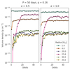 |
Fig. 13. Volume density variation in time in a given volume of Δr = 1 Req, Δϕ = 0.2 rad, and Δz = 4Req, centered on ϕ, z = 0) for models 50-0.5-0.16 and 50-1.0-0.16. |
To ascertain whether a disk is truly fully built up and thus subject to strong influence by a companion, regular monitoring of the Be star is necessary. Spectroscopy is particularly interesting, as the Balmer emission lines are the clearest indicators of disk development, and can be acquired by amateur astronomers with modest equipment for the brightest targets. Amateurs have contributed immensely to Be star databases such as BESS5.
Although more slowly than their build-up, Be disks also dissipate in relatively short timescales (Rímulo et al. 2018). When the injection of mass and AM from the central star stops, the disk dissipates inside-out (Haubois et al. 2012). Therefore, the inner Be and spiral dominated disk will be the first regions to be affected: as they are depleted, their contribution in the observables also diminish. The circumsecondary region, on the other hand, will take longer to feel the effects of the halting of mass and AM injection. As the matter around the secondary is bound to it, and will eventually be accreted. If the system is observed at this point in its evolution, the detection of the circumsecondary material (and of the secondary itself), is more likely, as its observable contribution is no longer drowned out by the Be disk. In their observations of the Be binary π Aqr during a phase of disk dissipation, Bjorkman et al. (2002) detected radial velocity shifts in Hα that were not compatible with the motion of the Be disk, but rather from a source outside of it. The authors attribute the emission to a cloud of gas around the companion, namely, the circumsecondary region. Observing dissipating Be disks that had previously been fed for a long period of time offers, therefore, the opportunity to detect faint companions in Be systems.
5. Conclusions
While interacting binary systems are well studied in literature, binary Be stars are unique systems given the nature of their decretion disks. In this work, we detail the structure and kinematics of Be stars in coplanar, circular binary systems using SPH simulations with unprecedented resolution, exploring orbital periods, mass ratios, and disk viscosity.
We identified five regions of the system with different characteristics and observational signatures:
-
Inner Be disk: innermost region of the decretion disk around the Be star, whose size depends strongly on the period and viscosity parameter of the disk. For less viscous disks, the accumulation effect is very significant; this denser disk would lead to stronger emission in lines that are formed in this region, such as Fe lines, as well as large polarization and infrared excess levels.
-
Spiral dominated disk: the influence of the secondary on the kinematics of the disk leads to the formation of a double armed density wave, more prominent and tightly wound the less viscous the disk. The observational effects of the waves are V/R variations in emission lines, in particular Hα and Hβ. The amplitude variation of the density waves decreases with binary separation, which likely leads to a correlation between V/R amplitude with orbital period, such as the one recently found by Miroshnichenko et al. (2023).
-
Bridge: the Be disk is not completely truncated by the tidal interaction with the secondary. What takes place is in fact more similar to Roche lobe overflow, where the decretion disk fills the lobe of the Be star, and matter is transferred to the lobe of the companion. The bridge is this connection between the two lobes, an extension of the leading spiral arm. Observationally, we expect to see asymmetries and features in absorption or emission lines, particularly in shell stars.
-
Circumsecondary region: matter that enters the RL of the companion is partially accreted and partially lost to the circumbinary region, escaping through the L2 point. The accretion rate is higher the smaller the relative velocity of the material that enters the RL to the companion. Depending on the density of the accretion disk of the companion, emission lines can be excited, which will behave differently from the Be disk lines. All of our simulations form disk-like (i.e., symmetric in density and rotationally supported) structure in this region.
-
Circumbinary spiral: outside of the orbit of the companion, material that escapes the system through the L2 and L3 points spirals together in a large one armed wave that encompasses the whole system. Although the spiral has very low density, continuum emission in radio wavelengths (and possibly in the far IR) is possible.
This five-region structure was predicted observationally by Peters et al. (2016) and by the SPH simulations of Panoglou et al. (2016), but this is the first work to show these structures forming in an SPH simulation of a Be binary system from first principles. The circumsecondary region has been confirmed by spectroscopic and/or interferometric observations to exist in a handful of systems (HR 2142 – Peters et al. (2016), Klement et al. (2024), HD5560 – Chojnowski et al. (2018), o Pup – Miroshnichenko et al. (2023), π Aqr – Bjorkman et al. (2002), and V658 Car – de Amorim, priv. comm.). The bridge and circumbinary spiral are less constrained. Our simulations confirm that these complex structures can be responsible for peculiar observational behavior of some known binary Be stars. The velocities of the absorption features seen in the intermittent shell phases of Be+sdO HR 2142 are compatible with what we see in the bridge in our models. The complex features seen in the spectra of Be+sdO HD 55606 might also come from the bridge or from the circumsecondary disk. Phase-dependent traveling features like these, observed in both absorption and emission in other Be stars, may indicate binarity according to our results. Radio excess found in Be binaries that also present SED turndown is a tentative indicator of the presence of diffuse material around the system, likely the circumbinary spiral seen in our simulations.
The significance of the regions described here for the spectroscopic appearance of the system depends on the evolutionary state of the disk, which is influenced by the viscosity, the variability of the Be star mass ejection, and the duration of the outburst phase. For a given orbital period and viscosity parameter, it can take years for the bridge, circumsecondary and circumbinary structures to be formed. Thus, any attempt to observe the expected observational effects we describe should take the disk evolution into account.
In an expansion of this work, we plan to include radiative transfer calculations with HDUST to our SPH models. This will provide synthetic photometry, spectroscopy, polarimetry, and interferometry data that can be directly compared to observations. This planned study will provide constraints for the observational detection and characterization of binary Be stars.
γ Cas, FR CMa, HR 2370, V558 Lyr, V782 Cas, and π Aqr.
Most simulations have a mass ratio of 0.16, based on Bjorkman et al. (2002). We note, however, that since the start of our work, the mass of the companion of π Aqr has been put to question by Tsujimoto et al. (2023), who finds M2 < 1.4 M⊙ in contrast with Bjorkman et al. (2002)’s M2 = 2.06 M⊙.
We note that most of the cited works use n, the volume density slope, instead of m, the surface density slope. They are related as n = m + β, where β = 1.5 for isothermal VDD disks.
See Dulaney et al. (2017) and Miroshnichenko et al. (2023) versus Harmanec et al. (2019) for the two opposing views on β CMi’s binarity.
Acknowledgments
A.C.R. acknowledges support from the ‘Coordenação de Aperfeiçoamento de Pessoal de Nível Superior’ (CAPES grant 88887.464563/2019-00), ‘Deutscher Akademischer Austauschdienst’ (DAAD grant 57552338), the ESO Studentship program (in particular Dr. Dietrich Baade and Dr. Antoine Mérand), and the Max Planck Institut für Astrophysik in Garching, Germany. A.C.C. acknowledges support from CNPq (grant 314545/2023-9) and ‘Fundação de Amparo à Pesquisa do Estado de São Paulo’ (FAPESP grants 2018/04055-8 and 2019/13354-1). J.E.B. acknowledges support from NSF grant AST-1412135. C.E.J. acknowledges support through the National Science and Engineering Research Council of Canada. M.W.S. acknowledges support via the Ontario Graduate Scholarship program T.H.A. acknowledges support from FAPESP (grant 2021/01891-2) and CAPES (grant 88887.834998/2023-00). This study was granted access to and greatly benefited from the HPC resources of: Centro de processamento de Dados do IAG/USP (CPD-IAG), whose purchase was made possible by the Brazilian agency FAPESP (grants 2019/25950-8, 2009/54006-4).
References
- Anugu, N., Le Bouquin, J.-B., Monnier, J. D., et al. 2020, AJ, 160, 158 [NASA ADS] [CrossRef] [Google Scholar]
- Armitage, P. J. 2011, ARA&A, 49, 195 [Google Scholar]
- Baade, D., Labadie-Bartz, J., Rivinius, T., & Carciofi, A. C. 2023, A&A, 678, A47 [NASA ADS] [CrossRef] [EDP Sciences] [Google Scholar]
- Bate, M. R., Bonnell, I. A., & Price, N. M. 1995, MNRAS, 277, 362 [Google Scholar]
- Benz, W., Bowers, R. L., Cameron, A. G. W., & Press, W. H. 1990, ApJ, 348, 647 [Google Scholar]
- Binney, J., & Tremaine, S. 2008, Galactic Dynamics, 2nd edn. (Princeton: Princeton University Press) [Google Scholar]
- Bjorkman, J. E. 1997, in Stellar Atmospheres: Theory and Observations, eds. J. P. De Greve, R. Blomme, & H. Hensberge (Berlin: Springer Verlag), Lecture Notes in Physics, 497, 239 [Google Scholar]
- Bjorkman, J. E., & Carciofi, A. C. 2005, in The Nature and Evolution of Disks Around Hot Stars, eds. R. Ignace, & K. G. Gayley, ASP Conf. Ser., 337, 75 [NASA ADS] [Google Scholar]
- Bjorkman, K. S., Miroshnichenko, A. S., McDavid, D., & Pogrosheva, T. M. 2002, ApJ, 573, 812 [Google Scholar]
- Bodenheimer, P. 1971, ApJ, 167, 153 [Google Scholar]
- Bodensteiner, J., Shenar, T., & Sana, H. 2020, A&A, 641, A42 [NASA ADS] [CrossRef] [EDP Sciences] [Google Scholar]
- Boubert, D., & Evans, N. W. 2018, MNRAS, 477, 5261 [Google Scholar]
- Carciofi, A. C. 2011, in IAU Symposium, eds. C. Neiner, G. Wade, G. Meynet, & G. Peters, 272, 325 [NASA ADS] [Google Scholar]
- Carciofi, A. C., & Bjorkman, J. E. 2006, ApJ, 639, 1081 [Google Scholar]
- Carciofi, A. C., & Bjorkman, J. E. 2008, ApJ, 684, 1374 [Google Scholar]
- Carciofi, A. C., Okazaki, A. T., Le Bouquin, J.-B., et al. 2009, A&A, 504, 915 [NASA ADS] [CrossRef] [EDP Sciences] [Google Scholar]
- Chojnowski, S. D., Labadie-Bartz, J., Rivinius, T., et al. 2018, ApJ, 865, 76 [NASA ADS] [CrossRef] [Google Scholar]
- Cranmer, S. R. 2005, ApJ, 634, 585 [NASA ADS] [CrossRef] [Google Scholar]
- Curé, M., Meneses, R., Araya, I., et al. 2022, A&A, 664, A185 [NASA ADS] [CrossRef] [EDP Sciences] [Google Scholar]
- Cyr, I. H., Jones, C. E., Panoglou, D., Carciofi, A. C., & Okazaki, A. T. 2017, MNRAS, 471, 596 [NASA ADS] [CrossRef] [Google Scholar]
- Cyr, I. H., Jones, C. E., Carciofi, A. C., et al. 2020, MNRAS, 497, 3525 [NASA ADS] [CrossRef] [Google Scholar]
- Dallas, M. M., Oey, M. S., & Castro, N. 2022, ApJ, 936, 112 [NASA ADS] [CrossRef] [Google Scholar]
- de Almeida, E. S. G., Meilland, A., Domiciano de Souza, A., et al. 2020, A&A, 636, A110 [NASA ADS] [CrossRef] [EDP Sciences] [Google Scholar]
- de Mink, S. E., Langer, N., Izzard, R. G., Sana, H., & de Koter, A. 2013, ApJ, 764, 166 [Google Scholar]
- Dodd, J. M., Oudmaijer, R. D., Radley, I. C., Vioque, M., & Frost, A. J. 2024, MNRAS, 527, 3076 [Google Scholar]
- Dulaney, N. A., Richardson, N. D., Gerhartz, C. J., et al. 2017, ApJ, 836, 112 [NASA ADS] [CrossRef] [Google Scholar]
- Edgar, R. 2004, New Astron. Rev., 48, 843 [CrossRef] [Google Scholar]
- Eggleton, P. P. 1983, ApJ, 268, 368 [Google Scholar]
- Ekström, S., Meynet, G., Maeder, A., & Barblan, F. 2008, A&A, 478, 467 [Google Scholar]
- Franchini, A., Martin, R. G., & Lubow, S. H. 2019, MNRAS, 485, 315 [NASA ADS] [CrossRef] [Google Scholar]
- Frank, J., King, A., & Raine, D. J. 2002, Accretion Power in Astrophysics, 3rd edn. (Cambridge: Cambridge University Press) [Google Scholar]
- Georgy, C., Ekström, S., Granada, A., et al. 2013, A&A, 553, A24 [NASA ADS] [CrossRef] [EDP Sciences] [Google Scholar]
- Gies, D. R., Bagnuolo, W. G., Jr., Ferrara, E. C., et al. 1998, ApJ, 493, 440 [NASA ADS] [CrossRef] [Google Scholar]
- GRAVITY Collaboration (Abuter, R., et al.) 2017, A&A, 602, A94 [NASA ADS] [CrossRef] [EDP Sciences] [Google Scholar]
- Hanuschik, R. W., Hummel, W., Sutorius, E., Dietle, O., & Thimm, G. 1996, A&AS, 116, 309 [NASA ADS] [CrossRef] [EDP Sciences] [Google Scholar]
- Harmanec, P., Švanda, M., Korčáková, D., et al. 2019, ApJ, 875, 13 [NASA ADS] [CrossRef] [Google Scholar]
- Hastings, B., Langer, N., Wang, C., Schootemeijer, A., & Milone, A. P. 2021, A&A, 653, A144 [NASA ADS] [CrossRef] [EDP Sciences] [Google Scholar]
- Haubois, X., Carciofi, A. C., Rivinius, T., Okazaki, A. T., & Bjorkman, J. E. 2012, ApJ, 756, 156 [Google Scholar]
- Haubois, X., Mota, B. C., Carciofi, A. C., et al. 2014, ApJ, 785, 12 [NASA ADS] [CrossRef] [Google Scholar]
- Hayasaki, K., & Okazaki, A. T. 2004, MNRAS, 350, 971 [NASA ADS] [CrossRef] [Google Scholar]
- Huang, W., Gies, D. R., & McSwain, M. V. 2010, ApJ, 722, 605 [Google Scholar]
- Kee, N. D., Owocki, S., & Sundqvist, J. O. 2016, MNRAS, 458, 2323 [Google Scholar]
- Keller, S. C., Bessell, M. S., Cook, K. H., Geha, M., & Syphers, D. 2002, AJ, 124, 2039 [Google Scholar]
- King, A. R., Pringle, J. E., & Livio, M. 2007, MNRAS, 376, 1740 [NASA ADS] [CrossRef] [Google Scholar]
- Kitsionas, S., & Whitworth, A. P. 2002, MNRAS, 330, 129 [Google Scholar]
- Klement, R., Carciofi, A. C., Rivinius, T., et al. 2015, A&A, 584, A85 [NASA ADS] [CrossRef] [EDP Sciences] [Google Scholar]
- Klement, R., Carciofi, A. C., Rivinius, T., et al. 2017, A&A, 601, A74 [NASA ADS] [CrossRef] [EDP Sciences] [Google Scholar]
- Klement, R., Carciofi, A. C., Rivinius, T., et al. 2019, ApJ, 885, 147 [Google Scholar]
- Klement, R., Baade, D., Rivinius, T., et al. 2022, ApJ, 940, 86 [NASA ADS] [CrossRef] [Google Scholar]
- Klement, R., Rivinius, T., Gies, D. R., et al. 2024, ApJ, 962, 70 [NASA ADS] [CrossRef] [Google Scholar]
- Kluska, J., Van Winckel, H., Coppée, Q., et al. 2022, A&A, 658, A36 [NASA ADS] [CrossRef] [EDP Sciences] [Google Scholar]
- Krtička, J., Owocki, S. P., & Meynet, G. 2011, A&A, 527, A84 [NASA ADS] [CrossRef] [EDP Sciences] [Google Scholar]
- Kurfürst, P., Feldmeier, A., & Krtička, J. 2018, A&A, 613, A75 [NASA ADS] [CrossRef] [EDP Sciences] [Google Scholar]
- Larsen, C., Larsen, H. C. G., Pedersen, C. C., et al. 2024, Nature, 625, E18 [Google Scholar]
- Lee, U., Osaki, Y., & Saio, H. 1991, MNRAS, 250, 432 [Google Scholar]
- Liu, Q. Z., van Paradijs, J., & van den Heuvel, E. P. J. 2006, A&A, 455, 1165 [NASA ADS] [CrossRef] [EDP Sciences] [Google Scholar]
- Liu, J., Zhang, H., Howard, A. W., et al. 2019, Nature, 575, 618 [Google Scholar]
- Lopez, B., Lagarde, S., Petrov, R. G., et al. 2022, A&A, 659, A192 [NASA ADS] [CrossRef] [EDP Sciences] [Google Scholar]
- Lucy, L. B. 1977, AJ, 82, 1013 [NASA ADS] [CrossRef] [Google Scholar]
- Marr, K. C., Jones, C. E., Carciofi, A. C., et al. 2021, ApJ, 912, 76 [NASA ADS] [CrossRef] [Google Scholar]
- Marr, K. C., Jones, C. E., Tycner, C., Carciofi, A. C., & Silva, A. C. F. 2022, ApJ, 928, 145 [NASA ADS] [CrossRef] [Google Scholar]
- Martin, R. G., & Franchini, A. 2019, MNRAS, 489, 1797 [NASA ADS] [CrossRef] [Google Scholar]
- Martin, R. G., Nixon, C., Armitage, P. J., Lubow, S. H., & Price, D. J. 2014, ApJ, 790, L34 [Google Scholar]
- Martin, R. G., Lubow, S. H., Armitage, P. J., & Price, D. J. 2024, MNRAS, 530, 4148 [Google Scholar]
- Meilland, A., Millour, F., Kanaan, S., et al. 2012, A&A, 538, A110 [CrossRef] [EDP Sciences] [Google Scholar]
- Miroshnichenko, A. S., Chari, R., Danford, S., et al. 2023, Galaxies, 11, 83 [Google Scholar]
- Mohamed, S., & Podsiadlowski, P. 2007, in 15th European Workshop on White Dwarfs, eds. R. Napiwotzki, & M. R. Burleigh, ASP Conf. Ser., 372, 397 [Google Scholar]
- Monageng, I. M., McBride, V. A., Coe, M. J., Steele, I. A., & Reig, P. 2017, MNRAS, 464, 572 [NASA ADS] [CrossRef] [Google Scholar]
- Monaghan, J. J., & Gingold, R. A. 1983, J. Comput. Phys., 52, 374 [CrossRef] [Google Scholar]
- Mourard, D., Bério, P., Perraut, K., et al. 2017, J. Opt. Soc. Am. A, 34, A37 [NASA ADS] [CrossRef] [Google Scholar]
- Nazé, Y., Rauw, G., Smith, M. A., & Motch, C. 2022, MNRAS, 516, 3366 [CrossRef] [Google Scholar]
- Negueruela, I., & Okazaki, A. T. 2001, A&A, 369, 108 [NASA ADS] [CrossRef] [EDP Sciences] [Google Scholar]
- Okazaki, A. T. 1991, PASJ, 43, 75 [NASA ADS] [Google Scholar]
- Okazaki, A. T. 2001, PASJ, 53, 119 [Google Scholar]
- Okazaki, A. T. 2007, in Active OB-Stars: Laboratories for Stellare and Circumstellar Physics, eds. A. T. Okazaki, S. P. Owocki, & S. Stefl, ASP Conf. Ser., 361, 230 [Google Scholar]
- Okazaki, A. T., & Negueruela, I. 2001, A&A, 377, 161 [NASA ADS] [CrossRef] [EDP Sciences] [Google Scholar]
- Okazaki, A. T., Bate, M. R., Ogilvie, G. I., & Pringle, J. E. 2002, MNRAS, 337, 967 [NASA ADS] [CrossRef] [Google Scholar]
- Owocki, S. 2006, in Stars with the B[e] Phenomenon, eds. M. Kraus, & A. S. Miroshnichenko, ASP Conf. Ser., 355, 219 [Google Scholar]
- Panoglou, D., Carciofi, A. C., Vieira, R. G., et al. 2016, MNRAS, 461, 2616 [Google Scholar]
- Panoglou, D., Faes, D. M., Carciofi, A. C., et al. 2018, MNRAS, 473, 3039 [NASA ADS] [CrossRef] [Google Scholar]
- Panoglou, D., Borges Fernandes, M., Baade, D., et al. 2019, MNRAS, 486, 5139 [NASA ADS] [CrossRef] [Google Scholar]
- Peters, G. J., Gies, D. R., Grundstrom, E. D., & McSwain, M. V. 2008, ApJ, 686, 1280 [Google Scholar]
- Peters, G. J., Pewett, T. D., Gies, D. R., Touhami, Y. N., & Grundstrom, E. D. 2013, ApJ, 765, 2 [Google Scholar]
- Peters, G. J., Wang, L., Gies, D. R., & Grundstrom, E. D. 2016, ApJ, 828, 47 [Google Scholar]
- Pols, O. R., Cote, J., Waters, L. B. F. M., & Heise, J. 1991, A&A, 241, 419 [NASA ADS] [Google Scholar]
- Price, D. J., Wurster, J., Tricco, T. S., et al. 2018, PASA, 35, e031 [Google Scholar]
- Quirrenbach, A., Bjorkman, K. S., Bjorkman, J. E., et al. 1997, ApJ, 479, 477 [NASA ADS] [CrossRef] [Google Scholar]
- Reig, P. 2011, Ap&SS, 332, 1 [Google Scholar]
- Richardson, N. D., & Eldridge, J. J. 2024, Nature, 625, E24 [Google Scholar]
- Richardson, N. D., Pavao, C. M., Eldridge, J. J., et al. 2023, Nature, 614, 45 [Google Scholar]
- Rímulo, L. R., Carciofi, A. C., Vieira, R. G., et al. 2018, MNRAS, 476, 3555 [Google Scholar]
- Rivinius, T., Carciofi, A. C., & Martayan, C. 2013, A&ARv, 21, 69 [Google Scholar]
- Rivinius, T., Klement, R., Chojnowski, S. D., et al. 2025, A&A, 694, A172 [NASA ADS] [CrossRef] [EDP Sciences] [Google Scholar]
- Rubio, A. C., Carciofi, A. C., Ticiani, P., et al. 2023, MNRAS, 526, 3007 [CrossRef] [Google Scholar]
- Sana, H., de Mink, S. E., de Koter, A., et al. 2012, Science, 337, 444 [Google Scholar]
- Schaefer, G. H., Gies, D. R., Monnier, J. D., et al. 2010, AJ, 140, 1838 [NASA ADS] [CrossRef] [Google Scholar]
- Shakura, N. I., & Sunyaev, R. A. 1973, A&A, 24, 337 [NASA ADS] [Google Scholar]
- Shao, Y., & Li, X.-D. 2014, ApJ, 796, 37 [Google Scholar]
- Speri, L., Antonelli, A., Sberna, L., et al. 2023, Phys. Rev. X, 13, 021035 [NASA ADS] [Google Scholar]
- Suffak, M., Jones, C. E., & Carciofi, A. C. 2022, MNRAS, 509, 931 [Google Scholar]
- Suffak, M. W., Jones, C. E., Carciofi, A. C., & de Amorim, T. H. 2023, MNRAS, 526, 782 [Google Scholar]
- Suffak, M. W., Jones, C. E., & Carciofi, A. C. 2024, MNRAS, 527, 7515 [Google Scholar]
- Tsujimoto, M., Hayashi, T., Morihana, K., & Moritani, Y. 2023, PASJ, 75, 177 [NASA ADS] [CrossRef] [Google Scholar]
- Vieira, R. G., Carciofi, A. C., & Bjorkman, J. E. 2015, MNRAS, 454, 2107 [NASA ADS] [CrossRef] [Google Scholar]
- Vieira, R. G., Carciofi, A. C., Bjorkman, J. E., et al. 2017, MNRAS, 464, 3071 [NASA ADS] [CrossRef] [Google Scholar]
- Wang, L., Gies, D. R., & Peters, G. J. 2017, ApJ, 843, 60 [Google Scholar]
- Wang, L., Gies, D. R., & Peters, G. J. 2018, ApJ, 853, 156 [Google Scholar]
- Wang, L., Gies, D. R., Peters, G. J., et al. 2021, AJ, 161, 248 [Google Scholar]
- Waters, L. B. F. M., van der Veen, W. E. C. J., Taylor, A. R., Marlborough, J. M., & Dougherty, S. M. 1991, A&A, 244, 120 [NASA ADS] [Google Scholar]
- Wood, K., Bjorkman, K. S., & Bjorkman, J. E. 1997, ApJ, 477, 926 [Google Scholar]
- Zharikov, S. V., Miroshnichenko, A. S., Pollmann, E., et al. 2013, A&A, 560, A30 [NASA ADS] [CrossRef] [EDP Sciences] [Google Scholar]
- Zhu, Z., Hartmann, L., Gammie, C., & McKinney, J. C. 2009, ApJ, 701, 620 [CrossRef] [Google Scholar]
All Tables
All Figures
|
Fig. 1. Comparison of averaged surface density and disk height between the models detailed in Table 1. First panel shows the density normalized by the viscosity parameter; second panel shows the scale height H, and the last panel the number of particles in a given radial extent. The dashed vertical line represents the position of the secondary, which is the same for all simulations. The horizontal line in the bottom panel marks 50 particles. |
| In the text | |
|
Fig. 2. Surface density map of simulation 0.05-on. The overall density structure is qualitatively similar for all simulations calculated for this work, as sketched in Fig. 3. The black circle denotes the Be star, and the black star, the companion. The white circles and numbers mark the radial distance in Req. The three colored bands correspond to the main regions of interest: the wedge that contains the secondary (yellow), the wedge opposite to the secondary (blue), and a wedge that includes the bridge (green). |
| In the text | |
|
Fig. 3. Sketch view of the main regions of the binary Be system. The five main regions are the inner Be disk (pink), the spiral dominated disk (purple), the bridge (teal), the circumsecondary region (blue) and the circumbinary region (mauve). The main characteristics of each region are detailed in the text. |
| In the text | |
|
Fig. 4. Radial velocity maps for models 30-0.1-0.16 and 30-1.0-0.16. The black dot in the center represents the central Be star. The double spiral structure formed by the elongation of the orbits of the particles is visible in both maps. The over-density occurs in the apastron of the orbits of the particles, where the particles slow down. |
| In the text | |
|
Fig. 5. Surface density, radial velocity, azimuthal velocity, eccentricity of the particles’ orbits, and scale height varying with radius for models 30-1.0-0.16 and 30-0.1-0.16 in the leftmost panels, 30-1.0-0.16 and 84-1.0-0.16 for the middle panels, and 30-1.0-0.33 and 30-1.0-0.50 for the rightmost panels. The colors of the lines indicate the wedges along which the quantities are calculated, following Fig. 2: yellow is the wedge pointing to the secondary, blue is the wedge in the opposite direction, and green includes part of the stronger spiral arm. The dotted gray lines show the position of the secondary for the models compared in each column. |
| In the text | |
|
Fig. 6. Mean surface density, radial and azimuthal velocities for discrete wedges in ϕ of 0.125 radians each (from ϕ = −π to π, where ϕ = 0 is the direction that includes both the Be star and the secondary). The model parameters are indicated at the top of each column. The top and bottom plots compare models with low and high α, respectively. Dashed lines in the middle panel represent resonance radii close to the nodes (see text for details). |
| In the text | |
|
Fig. 7. Surface density as a function of ϕ, at different fixed radial distances from the Be star (shown by the colormap), for models 30-0.1-0.16 and 30-1.0-0.16 (top), and 84-0.1-0.16 and 84-1.0-0.16 (bottom). |
| In the text | |
|
Fig. 8. Projected velocities along the line of sight of an observer at ϕ = 18° (left) and ϕ = 350° (right), for model 84-0.5-0.16. The background black and white map show the surface density of the system. The various colored bands map out the projected velocities, while the dashed orange lines indicate the direction of the observer. The black circle denotes the Be star, and the black star, the companion. |
| In the text | |
|
Fig. 9. Density maps for models 30-1.0-0.16 and 30-1.0-0.33, showing the Roche equipotential contours and the Lagrangian points. The black circle marks the Be star, and the black star, the companion. |
| In the text | |
|
Fig. 10. Map of radial (in full colors) and azimuthal (contours) velocity for simulation 30-1.0-0.16. The gray xs mark the regions of highest density for that given radii, tracking the two spiral arms. The black half circle marks the Be star, and the black star denotes the companion. |
| In the text | |
|
Fig. 11. Map of the ratio of vϕ to vr in the reference frame of the secondary, indicated by a black star in the center. Cross section contour plots (at z = 0) of the volume density (log(ρ), in g cm−3, integrated from z = −10 to 10 Req) of the circumsecondary region are shown in black. The Be star is to the left, not shown. |
| In the text | |
|
Fig. 12. Accretion rates and X-ray luminosities for our models. In the first three panels, different colors indicate period, and q and α remain fixed. In the fourth panel, colors indicate q, and period and α are fixed. |
| In the text | |
|
Fig. 13. Volume density variation in time in a given volume of Δr = 1 Req, Δϕ = 0.2 rad, and Δz = 4Req, centered on ϕ, z = 0) for models 50-0.5-0.16 and 50-1.0-0.16. |
| In the text | |
Current usage metrics show cumulative count of Article Views (full-text article views including HTML views, PDF and ePub downloads, according to the available data) and Abstracts Views on Vision4Press platform.
Data correspond to usage on the plateform after 2015. The current usage metrics is available 48-96 hours after online publication and is updated daily on week days.
Initial download of the metrics may take a while.