Evolution of the radial interstellar medium metallicity gradient in the Milky Way disk since redshift ≈3

B. Ratcliffe; S. Khoperskov; I. Minchev; N. D. Lee; T. Buck; L. Marques; J. P. Bernaldez; L. Lu; M. Steinmetz

doi:10.1051/0004-6361/202452658

Home

All issues

Volume 698 (May 2025)

A&A, 698 (2025) A267

Full HTML

Open Access

Issue		A&A Volume 698, May 2025


Article Number		A267
Number of page(s)		19
Section		Galactic structure, stellar clusters and populations
DOI		https://doi.org/10.1051/0004-6361/202452658
Published online		20 June 2025

A&A, 698, A267 (2025)

Evolution of the radial interstellar medium metallicity gradient in the Milky Way disk since redshift ≈3

B. Ratcliffe¹^★, S. Khoperskov¹, I. Minchev¹, N. D. Lee²^,3, T. Buck⁴^,5, L. Marques¹, J. P. Bernaldez⁶^,1, L. Lu⁷^,8 and M. Steinmetz¹

¹ Leibniz-Institut für Astrophysik Potsdam (AIP), An der Sternwarte 16, 14482 Potsdam, Germany
² BIFOLD, Berlin Institute for the Foundations of Learning and Data, Berlin, Germany
³ Technische Universität Berlin, Berlin, Germany
⁴ Universität Heidelberg, Interdisziplinäres Zentrum für Wissenschaftliches Rechnen, Im Neuenheimer Feld 205, 69120 Heidelberg, Germany
⁵ Universität Heidelberg, Zentrum für Astronomie, Institut für Theoretische Astrophysik, Albert-Ueberle-Straße 2, 69120 Heidelberg, Germany
⁶ Friedrich-Schiller Universität Jena, 07737 Jena, Germany
⁷ Department of Astronomy, The Ohio State University, Columbus, 140 W 18th Ave, OH 43210, USA
⁸ Center for Cosmology and Astroparticle Physics (CCAPP), The Ohio State University, 191 W. Woodruff Ave., Columbus, OH 43210, USA

^★ Corresponding author.

Received: 18 October 2024
Accepted: 27 March 2025

Abstract

Context. Recent works have identified a way to recover the time evolution of a galaxy’s disk metallicity gradient from the shape of its age–metallicity relation. However, the success of the method is dependent on how the width of the star-forming region evolves over time, which in turn is dependent on a galaxy’s present day bar strength.

Aims. In this paper, we account for the time variation in the width of the star-forming region when deriving the interstellar medium (ISM) metallicity gradient evolution over time (∇[Fe/H](τ)), which provides more realistic birth radii estimates of Milky Way (MW) disk stars.

Methods. Using MW/Andromeda analogs from the TNG50 simulation, we quantified the disk growth of newly born stars as a function of present day bar strength to provide a correction that improves recovery of ∇[Fe/H](τ).

Results. In TNG50, we find that our correction reduces the median absolute error in recovering ∇[Fe/H](τ) by nearly 30%. To confirm its universality, we tested our correction on two galaxies from NIHAO-UHD and found the median absolute error is almost four times smaller even in the presence of observational uncertainties for the barred MW-like galaxy. Applying our correction to APOGEE DR17 red giant MW disk stars suggests the effects of merger events on ∇[Fe/H](τ) are less significant than originally found, and the corresponding estimated birth radii expose epochs when different migration mechanisms dominated.

Conclusions. Our correction to account for the growth of the star-forming region in the disk allows for better recovery of the evolution of the MW disk’s ISM metallicity gradient and, thus, more meaningful stellar birth radii estimates. With our results, we are able to recover the evolution of the ISM gradient, providing estimates for the total stellar disk radial metallicity gradient and key constraints to select MW analogs across redshift.

Key words: stars: abundances / Galaxy: disk / Galaxy: evolution

© The Authors 2025

Open Access article, published by EDP Sciences, under the terms of the Creative Commons Attribution License (https://creativecommons.org/licenses/by/4.0), which permits unrestricted use, distribution, and reproduction in any medium, provided the original work is properly cited.

This article is published in open access under the Subscribe to Open model. Subscribe to A&A to support open access publication.

1 Introduction

Present day chemical abundance patterns offer crucial insights into the past evolution of galaxies. For example, radial abundance gradients arise from the complex interaction of gas accretion, interstellar medium (ISM) enrichment, mixing, and feedback tied to stellar evolution. Understanding how these gradients evolve over time helps constrain the various physical processes governing galactic evolution. However, tracking the changes in abundance patterns within a galaxy is challenging because history becomes erased by ISM mixing. Nevertheless, thanks to the different measurements, the evolution of radial metallicity gradients in galaxies across a wide range of masses is now available up to high redshift.

The nearby massive galaxies universally show negative gradients (Vila-Costas & Edmunds 1992; Zaritsky et al. 1994; Ryder 1995; van Zee et al. 1998; Pilyugin et al. 2004, 2006; Pilyugin & Thuan 2007; Pilyugin et al. 2014; Moustakas et al. 2010; Gusev et al. 2012; Sánchez et al. 2014; Bresolin & Kennicutt 2015). This result agrees with models based on the standard inside-out scenario of disk formation, which predicts a relatively quick self-enrichment with oxygen abundances and an almost universal negative metallicity gradient (Boissier & Prantzos 1999, 2000). Though, at higher redshifts, metallicity gradients show considerable variation among galaxies (Cresci et al. 2010; Queyrel et al. 2012; Stott et al. 2014; Carton et al. 2018), where a notable fraction of galaxies exhibit shallow or even positive gradients.

Stars that formed in different regions and epochs of a galaxy eventually mixed and now reveal only the present day abundance distribution. In this context, the Milky Way (MW) provides a unique opportunity to unravel its past. Encoded in each star’s chemical composition is information regarding the star’s time and place of birth (Freeman & Bland-Hawthorn 2002; Ness et al. 2019; Ratcliffe et al. 2022), allowing for the detection and classification of accretion events (e.g. Helmi et al. 2018; Buder et al. 2022; Cunningham et al. 2022; Khoperskov et al. 2023a; Horta et al. 2023; Buder et al. 2024) as well as an investigation into the chemical evolution (e.g., Matteucci 2012; Minchev et al. 2018; Frankel et al. 2018; Lu et al. 2024; Prantzos et al. 2023; Ratcliffe et al. 2020, 2023, 2024b; Spitoni et al. 2024) and present day state (e.g., Hayden et al. 2015; Ratcliffe & Ness 2023; Hawkins 2023; Imig et al. 2023; Haywood et al. 2024; Khoperskov et al. 2024b; Griffith et al. 2024) of the MW disk.

While abundances contain a wealth of information on their own, one also needs to know when and where the stars were born in order to best understand the evolutionary history of the MW disk as a whole. Since stars radially migrate away from their birth sites due to interactions with transient spirals (e.g., Sellwood & Binney 2002; Roškar et al. 2008a; Schönrich & Binney 2009), the overlap of multiple pattern speeds (Minchev & Quillen 2006; Minchev & Famaey 2010; Marques et al. 2025), or a rapidly slowing down bar (Halle et al. 2015; Khoperskov et al. 2020; Wozniak 2020), a given location in the Galaxy can be comprised of stars with a variety of different birth radii depending on stellar age and metallicity (Minchev et al. 2018; Agertz et al. 2021; Carrillo et al. 2023). This causes mono-age abundance gradients measured in the present day to appear weaker than the environment the stars formed in (Pilkington et al. 2012a; Minchev et al. 2013; Kubryk et al. 2013; Renaud et al. 2025), and therefore radial migration must be taken into account when modeling the Galaxy’s enrichment (Francois & Matteucci 1993). Unfortunately, a star’s angular momentum can permanently change, making it impractical to trace the star’s orbit back to recover where it was born.

Recent works have leveraged the chemical homogeneity of stellar clusters (Bland-Hawthorn et al. 2010; Ness et al. 2022) to recover the birth radii of stars in the MW disk (e.g., Minchev et al. 2018; Frankel et al. 2018, 2019, 2020). As shown in observations (Ness et al. 2019; Sharma et al. 2022) and cosmological zoom-in simulations (Carrillo et al. 2023), stars in small bins of [Fe/H] and age have a small scatter in other abundances, indicating that these two variables alone can capture the primary evolution of the birth environment of the Galaxy. Leveraging this along with a linear birth metallicity gradient (which is found in observations Deharveng et al. 2000; Esteban et al. 2017; Arellano-Córdova et al. 2021, and simulations Vincenzo & Kobayashi 2018; Lu et al. 2022), stellar birth radii (R_birth) can be recovered if the time evolution of the metallicity gradient (∇[Fe/H](τ)) and projected central metallicity ([Fe/H](R = 0, τ)) are known (Kordopatis et al. 2015). Minchev et al. (2018) constructed a method that simultaneously recovered R_birth and the MW disk metallicity profile over time under the constraint that the resulting R_birth distributions should be physically meaningful. In discovering a linear relation between the scatter in [Fe/H] across age bins and the birth metallicity gradient evolution with cosmic time, Lu et al. (2024) was able to update this method so that recovering R_birth is fully self-consistent.

In the realm of TNG50 MW/M31 analogs, this method was found to work well in galaxies with stronger bars (Ratcliffe et al. 2024a). For galaxies with weaker bars, however, the metallicity gradient was typically unable to be recovered from the range in [Fe/H]. The ability to recover ∇[Fe/H](τ) from the scatter in [Fe/H] across age was found to depend on how the width of the star-forming region evolves with time; stronger barred galaxies tend to have only a minor increase in the region where stars are forming in their disk, while in weaker barred galaxies it can grow drastically (Ratcliffe et al. 2024a). Thus, to best capture the evolution of the metallicity profile, the growth of the disk needs to be accounted for (Mollá et al. 2019).

In this paper, we propose a correction in recovering the metallicity gradient that accounts for how the width of the starforming region varies with time as a function of present day bar strength. This theoretical advancement enables us not only to determine the birth radii of MW stars and constrain the amplitude of radial migration as a function of time and Galactocentric distance but also to trace the evolution of the radial metallicity gradient back to a redshift of ≈3. This approach bridges Galactic archaeology with nearby extragalactic and high-redshift observations, providing a more comprehensive view of the evolution of galaxies in general.

The paper is organized as follows. In Sects. 2 and 3 we describe the data and methods used in this work, with the correction described in Sect. 3.1. The results of applying our correction to both simulations and observational data are given in Sect. 4. In Sect. 5 we put our MW results into context and provide criteria to identify MW progenitors. We end with our conclusions in Sect. 6.

2 Data

We used data from two simulation suites – TNG50 and NIHAO-UHD – in addition to APOGEE DR17 MW red giant disk stars. The MW/M31-like galaxies from TNG50 were used to measure how much the width of the star-forming region grows over time as a function of present day bar strength. Two galaxies from NIHAO-UHD were used to show the success of the correction proposed in this paper to account for galactic growth when recovering the metallicity gradient from the scatter in [Fe/H] across age bins. Finally, we applied our correction to recover new estimates of stellar birth radii in the MW disk, which follow expectations of inside-out formation better.

2.1 TNG50 MW/M31 analogs

We analyzed MW/M31 analogs from the TNG50 cosmological simulation (Pillepich et al. 2019; Nelson et al. 2019a,b), which is the highest resolution run of the IllustrisTNG project (Pillepich et al. 2018; Marinacci et al. 2018; Naiman et al. 2018; Springel et al. 2018; Nelson et al. 2018, 2019b) run with the moving-mesh code AREPO (Springel 2010). Within TNG50 there are 198 MW/M31-like galaxies, and their data are publicly available.¹ These galaxies were chosen using the criteria presented in Pillepich et al. (2024) at redshift 0, which ensures that the galaxies (I) have disk-like morphology with spiral arms, (II) have a stellar mass in the range M_*(< 30 kpc) = 10^10.5–11.2 M_⊙, (III) have no other galaxy with stellar mass ≥10^10.5M_⊙ within 500 kpc, and (IV) have a halo total mass smaller than M_200c(host)< 10¹³ M_⊙. We used the redshift 0 bar strengths from Khoperskov et al. (2024a), which are peak values of m = 2 Fourier harmonics of the density distributions, and calculated the disk scale lengths by fitting an exponential profile to the radial stellar surface density distribution of the disk (see Appendix B). The TNG50 galaxies span a variety of bar strengths – from no bar to a very strong bar – with the MW most closely resembling the stronger barred galaxies in terms of present day stellar mass and star formation history (Khoperskov et al. 2024b). To allow for a direct comparison between each simulated galaxy and the MW, we scaled each TNG50 galaxy to have a disk scale length of 3.5 kpc and a rotational velocity of 238 km/s at 8 kpc (Bland-Hawthorn & Gerhard 2016). This scaling does not impact galactic properties such as bar strength. While scaling does influence the bar length, this metric is challenging to compare with the MW due to its variability – bar length can increase by up to 100% depending on the spiral structure and strength (Hilmi et al. 2020) – and because the MW’s velocity field is consistent with both a long bar accompanied by weak spirals and a shorter bar with stronger spirals (Vislosky et al. 2024). We also only considered the stellar disk, defined as R_birth < 15 kpc, R < 15 kpc, |z| < 1 kpc, |z_birth| < 1 kpc, ecc <0.5, and used stellar particles that were born and are currently bound to the galaxy. Following Ratcliffe et al. (2024a), we only examine the 178 galaxies that have a strong correlation (<−0.85) between [Fe/H] and R_birth in the most recent Gyrs of evolution.

2.2 NIHAO-UHD simulations

We used the galaxies g2.79e12 and g8.26e11 from the NIHAO-UHD simulation suite (Buck et al. 2019a, 2020), run using the smooth-particle hydrodynamics code GASOLINE2 (Wadsley et al. 2017). Both galaxies have MW-like mass, a boxy/peanut-shaped bulge, and have been studied extensively due to their similarity to the MW in terms of chemistry (Buck 2020; Buck et al. 2021; Ratcliffe et al. 2022; Wang et al. 2024), merger history (Buck et al. 2023), dark halo spin (Obreja et al. 2022) and satellite galaxy properties (Buck et al. 2019a). g2.79.e12 is the most MW-like in terms of its bar and spiral arms, whose properties have been studied and put in the context of the MW (Buck et al. 2018, 2019b; Hilmi et al. 2020; Vislosky et al. 2024; Marques et al. 2025). The bar strengths were estimated from the ratio of the amplitude of the m = 2 to m = 0 Fourier components of the stellar density, and found to be A₂/A₀ ≈ 0.4–0.5 for g2.79e12 (Figure 1 of Hilmi et al. 2020) and <0.1 for g8.26e11.

Similar to our TNG50 sample, we scaled the NIHAO-UHD galaxies to have a disk radial scale length of 3.5 kpc, and chose stellar disk particles by R_birth < 15 kpc, |z| < 1 kpc, |z_birth| < 1 kpc, and ecc < 0.5. We additionally selected stellar particles with |V_z,birth| < 50 km/s to minimize merger contamination. To best match our MW APOGEE sample, we used star particles between 4 < R < 12 kpc, and only considered a random sample of 160 000 stellar particles from each galaxy.

2.3 APOGEE DR17

To recover the metallicity profile with cosmic time and radius for the MW disk (and therefore, also stellar R_birth), we used data from the Sloan Digital Sky Survey IV (SDSS-IV; Blanton et al. 2017) APOGEE DR17 (Majewski et al. 2017; Abdurro’uf et al. 2022) catalog. Stellar parameters and abundances are processed by the APOGEE Stellar Parameter and Chemical Abundance Pipeline (ASPCAP; Holtzman et al. 2015; García Pérez et al. 2016; Jönsson et al. 2020). We additionally used orbital eccentricities from the astroNN catalog (Mackereth & Bovy 2018; Leung & Bovy 2019) and the recommended uncorrected Sharma model ages from the distmass catalog (Imig et al. 2023; Stone-Martinez et al. 2024). We selected disk (|z| < 1 kpc, ecc <0.5, |[Fe/H]| < 1) stars with small uncertainties ([Fe/H]_err < 0.05 dex, unflagged [Fe/H], log₁₀Age_{err; upper} > 0), and used red giant branch stars to avoid systematic abundance trends (2 < logg < 3.6, 4250 < T_eff < 5500 K). We also ensured to use only stars with parameters that are within the distmass training set by removing stars with bit 2 set. These cuts left us with 162 784 MW disk stars for our sample.

To illustrate the direct effect of the correction on the gradient, we also used the sample of red giant APOGEE DR17 disk stars from Ratcliffe et al. (2023). This sample has the same selection criteria as listed above, except it uses the age catalog of Anders et al. (2023).

3 Methods

3.1 Proposed correction

The goal of this work is to recover the birth metallicity gradient of the MW disk across time. As mentioned in the introduction, this gradient can be approximated as linear, as found in observations (Deharveng et al. 2000; Esteban et al. 2017; Arellano-Córdova et al. 2021) and some simulations (Vincenzo & Kobayashi 2018; Lu et al. 2022), not including a potentially metal-rich core (found in TNG50 Ratcliffe et al. 2024a and the MW Rix et al. 2024; Khoperskov et al. 2024b). While the existence of a bar may cause deviations from this linearity (e.g., Minchev et al. 2012), we expect these deviations to be minimal since star formation in the bar region is expected to be quenched, as found in simulations (Khoperskov et al. 2018; Ratcliffe et al. 2024a) and observations (Géron et al. 2024; Renu et al. 2025).

The metallicity gradient at a given lookback time (∇[Fe/H](τ)) can be written as $\nabla [F e / H] (τ) = \frac{Δ [F e / H] (τ)}{Δ R (τ)},$ $\[\nabla[\mathrm{Fe} / \mathrm{H}](\tau)=\frac{\Delta[\mathrm{Fe} / \mathrm{H}](\tau)}{\Delta \mathrm{R}(\tau)},\]$ (1)

where Δ[Fe/H](τ) is the difference between the maximum and minimum [Fe/H] at a given time τ, and ΔR(τ) is the width of the star-forming region at a given time τ. We are unable to accurately estimate Δ[Fe/H](τ) due to observational constraints, such as incompleteness and pipeline dependencies. However, the relative scatter in [Fe/H] (Range [Fe/H]) can be estimated from the 5–95%-tile range (Lu et al. 2024; Ratcliffe et al. 2024a) or the standard deviation in [Fe/H] (Ratcliffe et al. 2023) in different age bins. Both of these methods minimize contamination from outliers and capture the shape of Δ[Fe/H](τ) (see left panel of Figure C.2).

To recover ∇[Fe/H](τ), the method of Lu et al. (2024) assumes that the width of the star-forming region is constant with time, or ΔR(τ) = ΔR. However, Figure 1 clearly illustrates that ΔR(τ) grows with time and its evolution is dependent on the galaxy’s present day bar strength. This dependency arises from whether star formation occurs in the central region of a galaxy; while galaxies with different bar strengths show similar inside-out growth, weaker-barred galaxies continue to form stars in the inner regions of the disk whereas stronger-barred galaxies exhibit quenching in the bar region (see Figure 6 in Ratcliffe et al. 2024a). This halt in star formation therefore makes ΔR(τ) less variable over time, whereas for weaker-barred galaxies ΔR(τ) can increase by a factor of 10 (Figure 1).

Since each group of galaxies based on redshift 0 bar strength exhibits a distinct trend in an increasing ΔR(τ), the method to recover the metallicity gradient from the range in [Fe/H] needs to allow for this variation. We therefore propose using a smoothed version of ΔR(τ) from Figure 1 to correct for the non-constant width of the star-forming region. Smoothing the width of the star-forming region for each bar strength (measured every 0.2 Gyr) over 6 Gyr captures the overall shape of ΔR(τ) while minimizing the local variations that may be non-universal. Our results below are consistent for different smoothing bins. We wish to emphasize that we treat ΔR(τ) as a unitless variable that captures the varying radial region of where stars form in a galaxy over time; we do not assume a physical value for the width of the star forming region and it is not affected by the distribution of stars within that region.

Since the metallicity gradient and scatter are negatively correlated, this means that the normalized gradient and scatter are additive inverses; when the scatter is largest, the metallicity gradient is steepest (i.e., the most negative). We introduce the corrected metallicity scatter as $σ [F e / H] (age) \equiv \frac{Range [F e / H] (age)}{Δ R (age)},$ $\[\sigma[\mathrm{Fe} / \mathrm{H}](\text {age}) \equiv \frac{\text {Range}[\mathrm{Fe} / \mathrm{H}](\text {age})}{\Delta \mathrm{R}(\text {age})},\]$

and then the normalized scatter can be written as $\tilde{σ} [F e / H] (a g e) \equiv \frac{σ [F e / H] (age) - min (σ [F e / H] (age))}{max (σ [F e / H] (age)) - min (σ [F e / H] (age))} .$ $\[\widetilde{\sigma}[\mathrm{Fe} / \mathrm{H}](\mathrm{age}) \equiv \frac{\sigma[\mathrm{Fe} / \mathrm{H}](\text {age})-\min (\sigma[\mathrm{Fe} / \mathrm{H}](\text {age}))}{\max (\sigma[\mathrm{Fe} / \mathrm{H}](\text {age}))-\min (\sigma[\mathrm{Fe} / \mathrm{H}](\text {age}))}.\]$

Given the gradient is negative, we need 0 to represent the weakest gradient, and −1 to represent when the gradient is steepest. The normalization can be rewritten as follows: $\begin{aligned} \tilde{\nabla} [F e / H] (τ) & \equiv \frac{\nabla [F e / H] (τ) - min (\nabla [F e / H] (τ))}{max (\nabla [F e / H] (τ)) - min (\nabla [F e / H] (τ))} - 1 \\ \equiv \frac{\nabla [F e / H] (τ) - max (\nabla [F e / H] (τ))}{max (\nabla [F e / H] (τ)) - min (\nabla [F e / H] (τ))} . \end{aligned}$ $\[\begin{aligned}\widetilde{\nabla}[\mathrm{Fe} / \mathrm{H}](\tau) & \equiv \frac{\nabla[\mathrm{Fe} / \mathrm{H}](\tau)-\min (\nabla[\mathrm{Fe} / \mathrm{H}](\tau))}{\max (\nabla[\mathrm{Fe} / \mathrm{H}](\tau))-\min (\nabla[\mathrm{Fe} / \mathrm{H}](\tau))}-1 \\& \equiv \frac{\nabla[\mathrm{Fe} / \mathrm{H}](\tau)-\max (\nabla[\mathrm{Fe} / \mathrm{H}](\tau))}{\max (\nabla[\mathrm{Fe} / \mathrm{H}](\tau))-\min (\nabla[\mathrm{Fe} / \mathrm{H}](\tau))}.\end{aligned}\]$

As $\tilde{\nabla} [F e / H] (τ)$ $\[\widetilde{\nabla}[\mathrm{Fe} / \mathrm{H}](\tau)\]$ and $\tilde{σ} [F e / H] (a g e)$ $\[\widetilde{\sigma}[\mathrm{Fe} / \mathrm{H}](\mathrm{age})\]$ are additive inverses, we then have $\tilde{σ} [F e / H] (a g e) = - \tilde{\nabla} [F e / H] (τ),$ $\[\widetilde{\sigma}[\mathrm{Fe} / \mathrm{H}](\mathrm{age})=-\widetilde{\nabla}[\mathrm{Fe} / \mathrm{H}](\tau),\]$

or $\begin{aligned} \tilde{σ} [F e / H] (age) & = - \frac{\nabla [F e / H] (τ) - max (\nabla [F e / H] (τ))}{max (\nabla [F e / H] (τ)) - min (\nabla [F e / H] (τ))} \\ = \frac{\nabla [F e / H] (τ) - max (\nabla [F e / H] (τ))}{min (\nabla [F e / H] (τ)) - max (\nabla [F e / H] (τ))} . \end{aligned}$ $\[\begin{aligned}\widetilde{\sigma}[\mathrm{Fe} / \mathrm{H}](\text { age }) & =-\frac{\nabla[\mathrm{Fe} / \mathrm{H}](\tau)-\max (\nabla[\mathrm{Fe} / \mathrm{H}](\tau))}{\max (\nabla[\mathrm{Fe} / \mathrm{H}](\tau))-\min (\nabla[\mathrm{Fe} / \mathrm{H}](\tau))} \\& =\frac{\nabla[\mathrm{Fe} / \mathrm{H}](\tau)-\max (\nabla[\mathrm{Fe} / \mathrm{H}](\tau))}{\min (\nabla[\mathrm{Fe} / \mathrm{H}](\tau))-\max (\nabla[\mathrm{Fe} / \mathrm{H}](\tau))}.\end{aligned}\]$

Following Lu et al. (2024), we defined $b \equiv max (\nabla [F e / H] (τ))$ $\[\mathrm{b} \equiv \max (\nabla[\mathrm{Fe} / \mathrm{H}](\tau))\]$ $a \equiv min (\nabla [F e / H] (τ)) - max (\nabla [F e / H] (τ)),$ $\[\mathrm{a} \equiv \min (\nabla[\mathrm{Fe} / \mathrm{H}](\tau))-\max (\nabla[\mathrm{Fe} / \mathrm{H}](\tau)),\]$

which allowed us to rearrange the above equation to solve for ∇[Fe/H](τ): $\nabla [F e / H] (τ) = a \tilde{σ} [F e / H] (a g e) + b .$ $\[\nabla[\mathrm{Fe} / \mathrm{H}](\tau)=\mathrm{a} \widetilde{\sigma}[\mathrm{Fe} / \mathrm{H}](\mathrm{age})+\mathrm{b}.\]$ (2)

Thus, we have that the time evolution of the metallicity gradient is a linear function of the scatter in [Fe/H] across age after adjusting it for the growth of the star-forming region.

The MW disk birth gradient is expected to weaken with cosmic time (e.g., Prantzos et al. 2023), and therefore the gradient of the youngest stars in the MW can be used for variable b in Equation (2). The steepest gradient (a + b in Equation (2)), on the other hand, is unknown, though it can be visually inferred from the distribution of birth radii for solar neighborhood populations (Lu et al. 2024; Ratcliffe et al. 2023). In this work, we automated the determination of the steepest gradient, rather than the manual by-eye approach used in previous works. We found the optimal value by minimizing |R − R_birth| for the youngest (<2 Gyr) stars across the entire disk, where R_birth is derived following Section 3 from Ratcliffe et al. (2023): $R_{birth} = \frac{[F e / H] - [F e / H] (R = 0, τ)}{a \tilde{σ} [F e / H] (age) + b} .$ $\[\mathrm{R}_{\text {birth }}=\frac{[\mathrm{Fe} / \mathrm{H}]-[\mathrm{Fe} / \mathrm{H}](\mathrm{R}=0, \tau)}{\mathrm{a} \widetilde{\sigma}[\mathrm{Fe} / \mathrm{H}](\text { age })+\mathrm{b}}.\]$

The optimization is achieved by minimizing the objective function $min_{a < 0} {∥ R - \frac{[F e / H] - [F e / H] (R = 0, τ)}{a \tilde{σ} [F e / H] (a g e) + b} ∥}_{1} .$ $\[\min _{\mathrm{a}<0}\left\|\mathrm{R}-\frac{[\mathrm{Fe} / \mathrm{H}]-[\mathrm{Fe} / \mathrm{H}](\mathrm{R}=0, \tau)}{\mathrm{a} \widetilde{\sigma}[\mathrm{Fe} / \mathrm{H}](\mathrm{age})+\mathrm{b}}\right\|_{1}.\]$

We solve this minimization problem using the L-BFGS-B algorithm from scipy.optimize (Byrd et al. 1995), its default solver for bound-constrained minimization. We find the mean optimal steepest gradient is −0.142 dex/kpc across 100 Monte Carlo samples, which is slightly weaker than previously reported (see Section 4.2 for more discussion).

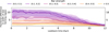Fig. 1

Illustration of how the median width of the star-forming region (and 25–75 percentile shaded region) in galaxies grows with cosmic time as a function of the present day bar strength using TNG50 MW/M31-like galaxies. Each line provides the fractional difference in the width of the star forming region, relative to a lookback time of 12 Gyr. In weaker-barred galaxies, where the width of the star-forming region increases by a factor of 10, the method of recovering the metallicity gradient from the range in [Fe/H] across age bins fails. When the width of the star-forming region does not change significantly over time (such as in the strongest barred galaxies), the method produces a smaller error. For the kilo-parsec values, we refer the reader to Figure C.3.

3.2 Denoising the age–metallicity relation

In this section, we show that denoising the age–metallicity plane before calculating Range [Fe/H](τ) is a necessary step in the realm of present day observational uncertainties in age. To make the best comparisons with the MW disk, we added error in age (15%) and [Fe/H] (0.05 dex) that is in line with observational uncertainties of current large spectroscopic surveys (e.g., Jönsson et al. 2020; Anders et al. 2023). The top panel of Figure 2 illustrates the structure in the age–metallicity plane of g2.79e12 that is lost due to observational uncertainty (see also Renaud et al. 2021b). In particular, the range in [Fe/H] is significantly larger at older ages for the data with uncertainties (blue) than the true data (gray). This increase in the [Fe/H] scatter is due to the larger age error for older age stars, along with the sharp change in [Fe/H] for increasing lookback time at the earlier stages of the disk. Therefore, this significant overestimation of Range [Fe/H] for age >8 Gyr is not found for the younger ages, and causes the recovered ∇[Fe/H](τ) to be too steep at larger lookback times, an issue not found when using the unperturbed data (see Appendix Figure C.4).

To tackle this problem caused by observational uncertainties, we denoised the age–metallicity relation using the nonparametric maximum likelihood estimator (NPMLE; Soloff et al. 2025)². The NPMLE recovers denoised estimates of parameters without assuming the data follow a specific underlying distribution. This allows for better estimates of complex data without simplifying the naturally intricate relationship between variables. The main details of the method are given in Appendix Section A. The denoised age–metallicity relation of g2.79e12 matches well the true distribution (middle panel of Figure 2). In particular, the shape in [Fe/H] for ages >8 Gyr is in much better agreement with the true data than the error-convolved data.

4 Recovering the ISM metallicity gradient from stellar age and [Fe/H]

4.1 Correcting for the growth of the star-forming region in simulations

4.1.1 Impact of the star-forming region growth correction in TNG50

As discussed in Section 3.1, we propose a correction to the measured scatter in [Fe/H] across age that takes the growth of the star-forming region into account by adjusting for ΔR(τ). The time evolution of ΔR(τ) depends on the galaxy’s present day bar strength; as a galaxy grows, quenching in the inner region of strongly barred galaxies (Khoperskov et al. 2018; Géron et al. 2024) creates a more constant ΔR(τ) with time, while weakly barred galaxies do not experience this halt in star formation, causing the width of the star-forming region to continually grow (Ratcliffe et al. 2024a). Therefore, the ΔR(τ) correction is chosen based on the galaxy’s redshift 0 bar strength (Figure 1, see also Figure C.3 in the Appendix).

To illustrate the power of our proposed correction, we first applied it to our TNG50 MW/M31 analogs sample. Figure 3 shows the correlation between ∇[Fe/H](τ) and Range[Fe/H](age) using the measured range (dashed lines) and adjusted range using our proposed correction (solid lines). A correlation close to −1 implies recovering the shape of ∇[Fe/H](τ) from Range[Fe/H](age) is successful, whereas a correlation near 0 or positive implies that the method would be unsuccessful. Each group of galaxies exhibits an overall improvement in their ability to have the gradient recovered from the scatter in [Fe/H] after our proposed adjustment, with the median correlation across all galaxies improving to −0.88. In particular, the galaxies with bar strength <0.4 show the largest improvement after applying our correction, with a peak in correlation now near −0.89.

Our correction to the method only minimally helped in stronger barred galaxies, as the method was already quite successful in this regime. The overall enhancement our correction produces in the method is also reflected in the median absolute percent error when estimating ∇[Fe/H](τ) from Range[Fe/H](age), which decreases from 28% to 20% across all galaxies.

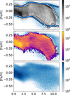Fig. 2

Role of denoising the age–metallicity relation in recovering the metallicity gradient from the scatter in [Fe/H] as a function of age. The age–metallicity relation for g2.79e12 (gray scale) with 15% age and 0.05 dex [Fe/H] uncertainty added (blue scale) is shown in the top panel. The horizontal lines correspond to the upper and lower bounds used to calculate Range [Fe/H] (age) measured with (blue) and without (white) measurement uncertainties. The range measured using the data with uncertainties is much larger than the range measured using the true age and [Fe/H] values for age >9 Gyr. The middle panel shows the distribution of the denoised ages (Section 3.2) and [Fe/H] (plasma) match well the age–metallicity relation of the true distribution. The presence of present day observational uncertainties (also shown in the bottom panel) makes denoising the age–metallicity relation a requirement to recover the structure in this plane, and thus Range [Fe/H] (age).

4.1.2 Confirming success with an independent simulation prescription – NIHAO-UHD

To demonstrate the correction we propose – which is based solely on TNG50 MW/M31 analogs – is not simulation-specific, we also show its success when recovering the gradient of MW-like galaxy g2.79e12 from NIHAO-UHD (Buck et al. 2020). To ensure the correction can be extended to the MW, we added uncertainties in age (15%) and [Fe/H] (0.05 dex). Since the range in [Fe/H] is overestimated at larger ages due to the uncertainties added (Section 3.2), we show the recovered gradients after denoising in age and [Fe/H] in Figure 4. For galaxy g2.79e12, ∇[Fe/H](τ) (red line) has an inversion ~10 Gyr ago caused by a GSE-like merger, and a strong flattening of the gradient with cosmic time afterward due to the bar rearranging stars on their orbits and mixing metal rich and metal poor stars in the disk before they enrich the ISM (Buck et al. 2023). Using the unmodified Range [Fe/H] (age) (gray line, as proposed in Lu et al. 2024) does a reasonable job of recovering the true evolution of the metallicity gradient; however, it significantly underestimates the gradient at older ages. This is because stars are forming on a smaller area at these higher lookback times than compared to the later stages of evolution (Figure 1), which causes the [Fe/H] range to be smaller than if stars were forming on a similar radial width of the disk over time. Similarly, the range for younger stars is artificially larger due to stars forming on a larger range of the disk. Applying our ΔR(τ) correction to adjust the range in [Fe/H] and account for this disk growth allows for a closer recovery of the truth in the stronger-barred galaxy (black line in the left panel of Figure 4). We find that the median absolute percent error after accounting for the time variation in the width of the star-forming region is nearly four times smaller than when no correction is applied.

In addition to a NIHAO-UHD galaxy with a stronger bar, we also tested our correction for galaxies with no bar. Figure 1 shows that the weaker-barred galaxies have a lot more variability in the growth of their star-forming region, particularly for galaxies with a bar strength <0.1. Our sample size for this regime of bar strength is also much smaller than the other groups. Thus, we combine bar strengths 0–0.2 into one group for our correction. The right panel of Figure 4 shows the recovered gradient for g8.26e11 with (black line) and without (gray line) correcting for the growth of the galactic disk. The correction gives an overall improvement to the recovered gradient, especially capturing the non-monotonic behavior. We also find that the gradient is estimated to be steeper than expected for 6–8 Gyr, indicating that the correction for weaker barred galaxies is less universal than suggested using our TNG50 sample (Figure 3). However, adjusting for ΔR in this regime can still provide helpful corrections to the gradient.

In this section we have demonstrated the success of our method on two MW-like galaxies with different formation histories and different morphologies than the ones used to create the ΔR(τ) correction. In g2.79e12 we see a strong flattening of the gradient with cosmic time due to the bar rearranging stars on their orbits and mixing metal rich and metal poor stars in the disk before they enrich the ISM, whereas in g8.26e11, the continued quiet star formation with a few late minor mergers leads to minimal evolution in the metallicity gradient (Buck et al. 2023). Thus, it is reassuring that our proposed correction to the gradient recovery method works well in a variety of evolutionary situations.

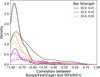Fig. 3

Correlation between the shape of the metallicity gradient over time and the range in [Fe/H] measured across age bins using the method with (solid lines) and without (dashed lines) our proposed correction applied for our sample of 178 TNG50 MW/M31-like galaxies. The colored lines correspond to the correlation of galaxies with different bar strengths, with the black line providing the density of the entire sample. A correlation of −1 implies that the shape of the gradient can be perfectly recovered from Range[Fe/H](age), and that the method is successful. With no correction applied, the median correlation is −0.74 (median absolute percent error of 28%), whereas when applying the correction the median correlation improves to −0.88 (median absolute percent error of 20%). The correction has a smaller improvement on stronger-barred galaxies (yellow) where the method already exhibited good success, but the correlation of galaxies with weaker present day bars show an improvement of over 40%.

4.2 Recovering the evolution of the MW disk metallicity gradient in the ISM

Now that we have established our proposed ΔR(τ) correction allows for a better recovery of ∇[Fe/H](τ), we extend it to the MW disk. We chose to apply the correction for galaxies with a bar strength of >0.5, as the MW closely resembles this category in the realm of TNG50 MW/M31-like galaxies, including the present day stellar mass and star formation history (Khoperskov et al. 2024a). Figure 5 compares the metallicity gradient recovered after applying the correction to our APOGEE samples with ages from distmass (solid black line with the shaded area showing the 25–75 percentile) and Anders et al. (2023) (blue line) to that of Ratcliffe et al. (2023) where no correction was applied (dashed line). The gradients in this work are taken as the mean ∇[Fe/H](τ) of 100 Monte Carlo samples, where both the age and [Fe/H] were drawn from a normal distribution about their measured values and a standard deviation of their measurement errors and then denoised. Since stars older than 10 Gyr are not well-represented in the distmass catalog (Imig et al. 2023), we estimate the gradient using a linear regression fit from the 8.6–9.6 Gyr data. The gradient recovered from distmass ages, including the estimation at older ages, is in good agreement with the gradient found using ages from Anders et al. (2023) after the correction is applied, with both gradients showing similar trends across time.

The overall trend of the newly recovered metallicity gradients is similar to what was previously reported in Ratcliffe et al. (2023); the gradient was steepest at ~9–10 Gyr ago and has been non-monotonically weakening with time. This overall flattening is in agreement with previous works deriving the metallicity gradient from observational data (Minchev et al. 2018; Lu et al. 2024; Ratcliffe et al. 2023) and additionally predictions from models such as Minchev et al. (2013); Prantzos et al. (2023); Chen & Prantzos (2025). However, due to the correction, we now find a much weaker gradient in the past ~8 Gyr, and a stronger gradient at older ages. The steepening phases found ~9 Gyr ago potentially due to Gaia-Sausage-Enceladus (GSE; Belokurov et al. 2018; Helmi et al. 2018, though see also Prantzos et al. 2023 for an argument for secular evolution) and 3 Gyr ago due to the Sagittarius dwarf galaxy (Ibata et al. 1994; Law & Majewski 2010) are still found, and suggest that these steepening events may be real as they are found across different surveys, stellar evolutionary phases, and age catalogs. While Ratcliffe et al. (2023) attributed these fluctuations to mergers (see also Buck et al. 2023), Prantzos et al. (2023) was able to produce an inversion in ∇[Fe/H](τ) ~ 9 Gyr ago solely through secular evolution. Additionally, Chen & Prantzos (2025) showed how recent star formation and intense infall episodes can create the “wiggly” behavior we observe in Figure 5 using a semi-analytical model with parametrized radial migration. Additionally, the steepening phase at ~6 Gyr ago found in Ratcliffe et al. (2023) using the Anders et al. (2023) (APOGEE DR17 red giant disk stars) and StarHorse (GALAH DR3 subgiant branch disk stars; Buder et al. 2021; Queiroz et al. 2023) age catalogs still exists after applying the correction to the Anders et al. (2023) ages; however, it has a much smaller impact. The lack of fluctuation found at this time using the distmass catalog suggests that the exponential age errors may have washed away the small feature³. A more detailed discussion of the MW disk ISM gradient evolution is given in Section 5.1, where the gradient is discussed in a broader context.

Figure 5 also provides the present day gradient measured using linear regression in the [Fe/H]–R_guide plane across different mono-age populations. The flat gradient of stars ⪆8 Gyr is when the correlation between [Fe/H] and R_guide significantly weakens; thus the gradient for these older ages captures a cloud-like structure rather than a true nearly flat gradient. Examining the present day gradient, we find three main epochs: 0–5 Gyr, 5–9 Gyr, and >9 Gyr. In the most recent 5 Gyr of evolution, we find that radial migration affects the metallicity gradient by weakening it ≲0.03 dex/kpc, suggesting that the MW disk has had quiescent evolution over the past ~5 Gyr. From 5–9 Gyr ago, we find a significant weakening of the present day stellar gradient, while for stars older than 9 Gyr (during the transition from the low- to high-α sequence) we find no [Fe/H]–R_guide structure. Comparing this to our recovered [Fe/H]–R_birth gradient (black and blue lines), we see that these epochs correspond with the steepening of the gradient potentially from Sagittarius and GSE (Annem & Khoperskov 2024; Buck et al. 2023).

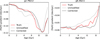Fig. 4

Demonstration of how the recovered [Fe/H] gradient using our proposed correction works in g2.79e12 (left; strong bar) and g8.26e11 (right; no bar) from the NIHAO-UHD simulation suite, which are completely independent of the TNG50 galaxies that are used to determine the correction. As discussed in Section 4.1.2, we added 0.05 dex and a 15% error to [Fe/H] and age and then denoised to make the best extensions to the MW. The black line in each panel represents the recovered metallicity gradient with the correction applied, and it matches the true [Fe/H] gradient evolution of disk stars (red line) better than recovering the metallicity gradient without the correction (gray line).

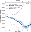Fig. 5

Comparing the recovered MW disk metallicity gradients with and without correcting for the growth of the star-forming region. The dashed gray line represents the gradient found in Ratcliffe et al. (2023) using ages from Anders et al. (2023), while ∇[Fe/H](τ) recovered using the correction proposed in this paper is shown in blue (ages from Anders et al. 2023) and gray (ages from distmass). The gradient is taken as the mean of 100 Monte Carlo samples where (age, [Fe/H]) are redrawn from a normal distribution and then denoised, and the shaded areas represent the 25–75 percentiles. The range in [Fe/H] is measured in age bin widths of 1 Gyr, taken every 0.2 Gyr. The corrected gradient recovered using the two different age catalogs is strikingly consistent and illustrates that the fluctuations in the gradient are not artifacts of the age catalog. The steepening events in the gradient ~8, ~6, and ~3 Gyr ago are less significant after the correction is applied; however, there is still non-monotonicity in the gradient’s evolution. We also provide the present day gradient (dashed purple line measured using R_guide) to illustrate the information lost due to radial migration.

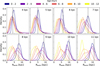Fig. 6

Birth radii distributions of the mono-age MW disk stars currently located within 0.25 dex of different radii (as indicated by the dashed black line in each panel) with |z| ≤ 0.5 kpc. The area under each mono-age curve is normalized to 1, so the curves are not representative of the relative proportion of each age at a given radii, but rather to illustrate the individual trends of each mono-age population. For each radial bin, the youngest population peaks within 0.5 kpc from where they are currently located today while each older population has consecutively smaller and smaller birth radii. Comparing the distribution of stars in the solar neighborhood (bottom left panel) to that of Ratcliffe et al. (2023), the correction used in this paper provides less migration for the 2–6 Gyr old populations and less spread in the oldest population.

4.2.1 Improved stellar birth radii for the MW disk

With our corrected ∇[Fe/H](τ) (Figure 5), we can recover improved stellar birth radii of MW disk stars. Just as in Lu et al. (2024) and Ratcliffe et al. (2023), the projected central metallicity is taken as the 95 percentile in [Fe/H] for older ages (age ≥10.75 Gyr) and estimated as monotonically increasing until its projected value at the present day assuming the youngest stars in the solar neighborhood have a metallicity of 0.06 (Nieva & Przybilla 2012; Asplund et al. 2021) and a gradient of −0.071 dex/kpc (Trentin et al. 2024). As shown in Ratcliffe et al. (2024a), nearly 50% of TNG50 galaxies exhibited a monotonic increase in their projected central metallicities, making this assumption a reasonable starting point. Though to understand its validity, we need to investigate the R_birth distributions of mono-age populations to see if they follow expectations of inside-out formation (Ratcliffe et al. 2024a).

Figure 6 shows the distribution of mono-age populations of stars currently located at different radii, as indicated by the dashed black line in each panel. Previously, only the distributions of mono-age populations in the solar neighborhood were used to confirm if the birth radii seemed reasonable. Here, we now ensure that the distributions of mono-age populations are reasonable for stars currently located at a variety of radii throughout the Galactic disk. At each radius, the youngest stars are born predominantly within 0.5 kpc of where they are currently located, and the older stars peak at progressively smaller birth radii in agreement with expectations from inside-out formation (e.g., Minchev et al. 2014; Agertz et al. 2021; Ratcliffe et al. 2024a). This clear sign of inside-out formation indicates that our choice for a monotonically increasing projected central metallicity is validated. While there may be small deviations from its monotonicity – which in turn would cause the corresponding R_birth distributions to slightly shift to lower radii – there is currently no way to improve this estimate without making assumptions about the chemical enrichment of the disk, such as the effect of mergers on the projected central metallicity, which is non-universal (Ratcliffe et al. 2024a).

The birth radii recovered in this work also show less migration than Lu et al. (2024); Ratcliffe et al. (2023), particularly for the middle-aged populations. The oldest population also exhibits less spread in birth radii than in Ratcliffe et al. (2023), though it does contain negative birth radii. One possibility for this is that these older stars are both not well represented in the data and also have the largest age uncertainties, and therefore, the upper envelope used to estimate the projected central metallicity at these older ages may not adequately capture the true distribution of the projected central metallicity. However, these negative birth radii make up less than 0.1% of our R_birth estimates, which is very minimal contamination.

We can now also get an improved estimate of the birth radius of the Sun. Assuming [Fe/H]_Sun = 0 ± 0.05 dex (Asplund et al. 2009) and age_Sun = 4.57 ± 0.11 Gyr (Bonanno et al. 2002), we estimate the Sun’s birth radius as 6.46 ± 0.59 kpc. This result is coincidentally in agreement with that found by Wielen et al. (1996), who estimated this value simply from the difference in [Fe/H] of the Sun versus other stars in the solar neighborhood and assuming a constant metallicity gradient with time. Our estimate is in the middle of other solar birth radius estimates, which range from 4.5 kpc to 7.8 kpc (Kubryk et al. 2015; Frankel et al. 2018; Minchev et al. 2018; Frankel et al. 2020; Lu et al. 2024; Baba et al. 2023; Prantzos et al. 2023; Chen & Prantzos 2025).

Table 1

Median migration distance for stars of different ages and guiding radii.

4.2.2 Migration strength in the MW disk

With estimates of stellar birth radii in the MW disk, we can probe the migration strength of the MW over time. Table 1 presents our recovered median migration distance as a function of stellar age and guiding radius, where a negative value corresponds to inward migration (i.e., R_birth > R_guide). We find a net outward median migration distance of 1.6 kpc for our sample, with more migration for older stars (in agreement with the effect of heating found in simulations; Minchev et al. 2014). The radius change root mean square of our sample $(\sqrt{m e a n {(R_{g u i d e} - R_{b i r t h})}^{2}})$ $\[(\sqrt{{mean}\left(R_{{guide}}-R_{{birth}}\right)^{2}})\]$ is 2.9 kpc. While this value is in agreement with migration strengths reported in simulations (Roškar et al. 2008b; Beraldo e Silva et al. 2021; Khoperskov et al. 2021) and other MW disk studies (Frankel et al. 2020), we stress that there is degeneracy in this value, as the causes of migration and their relative proportions can be different.

Similar to the three epochs found in the present day gradient measured using guiding radii (Section 4.2), we also observed three phases in the median migration strength with our estimated stellar birth radii. For stars with ages ≲ 6, we find minimal (<1.5 kpc) net outward migration and smaller root mean square change in radius (<2.1 kpc). This is a direct result of the more quiescent picture we described above, where the difference between the present day gradient and recovered birth gradient only minimally vary. Thus, the migration found here is probably driven by internal perturbations. From 6–10 Gyr ago, we find slightly more migration than in the more recent times (root mean square change in radius of 3.58 kpc). This extra migration period burst may be due to Sagittarius, or, since it has been shown that most migration happens within a few Gyr of beginning of bar formation (Minchev et al. 2011; Khoperskov et al. 2020), our results could suggest that the MW bar formed ~8–10 Gyr ago (in agreement with other independent findings; e.g., Bovy et al. 2019; Haywood et al. 2024; Sanders et al. 2024). The oldest stars of our sample experience the most migration (root mean square radius change 4.2 kpc). Disentangling the sources of this migration is impossible, as it can be due to many different causes over time (GSE, Sagittarius, bar, spiral arms).

Across R_guide, we find net inward migration for stars currently located in the inner disk, and net outward migration for stars R_guide > 5 kpc, as expected from numerical simulations (e.g., Minchev et al. 2014, Fig. 3). We estimate that ~44% of the stars in R_guide < 5 kpc are inward migrators – which we define as R_birth − R_guide > 2 − whereas the outer disk (9 < R_guide < 11 kpc) contains ~38% outward migrators. Looking across all ages, stars currently located in the solar neighborhood (7 < R_guide < 9 kpc) have, on average, experienced the most net migration. However, this conclusion is a bit misleading, as most mono-age bins show more net migration for larger R_guide (in agreement with simulations; Renaud et al. 2025). Therefore, we suggest that readers focus on the migration distance as a function of both age and guiding radius, and not marginalize over age.

5 Putting the evolution of metallicity gradients in the MW disk into context

5.1 ISM metallicity gradient

In this section, we use the derived birth radii of MW disk stars to constrain the evolution of radial metallicity gradients up to redshift ~3. The solid black and blue lines in Fig. 5 illustrate the birth radial metallicity gradient as a function of stellar age, which is equivalent to the evolution of the radial metallicity gradient in the star-forming ISM. Similar quantities are measured in large amounts for extragalactic systems, where the negative gradients dominate in disk galaxies at low redshifts (Ho et al. 2017a,b). However, the data for z > 1 show a diverse picture with a large scatter from negative to flat and even positive gas metallicity gradients (Stott et al. 2014; Wuyts et al. 2016; Leethochawalit et al. 2016; Venturi et al. 2024). Simulations allow one to somewhat resolve this complexity, suggesting that strong negative metallicity gradients mostly appear in galaxies with a gas disk, as reflected by well-ordered rotation (Ma et al. 2017; Pilkington et al. 2012b; Gibson et al. 2013). Since the MW disk is believed to assemble quite early (z > 3; Belokurov & Kravtsov 2022; Xiang & Rix 2022; Semenov et al. 2024b), we may expect that it has a steep metallicity gradient. We note that this assumption is behind the birth radii calculation (Minchev et al. 2018), trivially requiring the existence of the disk component. The birth radii determination assumes that stars in our sample correspond to the disk populations; however, contamination of accreted stars, especially for stars older than 8–10 Gyr is known (Di Matteo et al. 2019; Belokurov et al. 2020). The disentangling of accreted from in situ (genuine disk) stars is quite complex and not a fully resolved problem (Buder et al. 2022; Khoperskov et al. 2023b; Carrillo et al. 2024); however, we can safely neglect a small possible fraction of ex situ populations as we do not use stars with metallicities <−1 and eccentricity >0.5 for the birth radii and abundance gradients calculation.

To make meaningful comparisons with extragalactic observations, it is essential to ensure that the gradients are compared to MW analogs at corresponding redshifts. In the left panel of Figure 7, we show the redshift evolution of the radial metallicity gradient in the star-forming ISM color coded with MW stellar mass, whose time variation was adapted from Snaith et al. (2015), who recovered the MW mass-growth using chemical abundance patterns in the disk.

The left panel of Figure 7 also provides the ISM gradients of external galaxies (Queyrel et al. 2012; Simons et al. 2021; Wuyts et al. 2016; Förster Schreiber et al. 2018; Li et al. 2022; Ju et al. 2025) together with the compilation of TNG50 data from Hemler et al. (2021) (asterisks for the peak of the metallicity gradient distribution and gray are for the range) and a barred galaxy metallicity gradient from the NIAHO-UHD sample (Buck et al. 2023). There is a large scatter in observed metallicity gradients at a given redshift, with many galaxies showing flat or positive radial gradients. While our recovered MW gradient is on the steeper side when compared with these external galaxies, it is still within the spread we observe.

The evolution of the star-forming gas metallicity gradient in the MW is quite monotonic (see left panel of Figure 7), in general agreement with a flattening over time predicted in chemical evolution models (Mollá et al. 1997; Portinari et al. 1998; Hou et al. 2000). There is little gradient variation from z ~ 3 to z ~ 1 where it remains rather steep (≈ −0.14 dex/kpc). This epoch is characterized by the most intense phase of star formation when about half of the MW stellar mass was formed. Our birth radii suggest that the star-forming region is likely confined to the inner ≈6 kpc during this time (Figure 6). The steep metallicity gradient during this evolutionary phase is somewhat surprising, as the high star formation rate would imply a high rate of turbulence and mixing, effectively erasing the radial structure of the metallicity distribution (Brook et al. 2004, 2005; Bournaud et al. 2009). Ma et al. (2017), however, suggest that the metallicity gradient remains flat in such a bursty star formation regime if the galaxy remains clumpy with little rotation, which is not the case in the MW (Belokurov & Kravtsov 2022; Khoperskov et al. 2024a; Conroy et al. 2022; Semenov et al. 2024a). Using the VINTERGATAN simulation (Agertz et al. 2021; Renaud et al. 2021b,a), Segovia Otero et al. (2022) showed that a high rate of star formation is possible once the rotationally supported disk is settled. Therefore, the current state of the debate about the existence (and the strength) of the radial metallicity gradient at early phases of the MW-like galaxies remains open, as different galaxy formation models and subgrid physics can provide us with different solutions. At the same time, the extragalactic observations favor a steep gradient at high redshift for already rotationally supported galaxies (Jones et al. 2013, 2015).

The next feature in the gas metallicity gradient evolution is the non-monotonic change around z ~ 1.5–1 (see Fig. 7, left panel). As already anticipated, this epoch corresponds to the infall of the GSE (Belokurov et al. 2018; Haywood et al. 2019) and simultaneously the end of the high-α, inner disk formation (see, e.g., Haywood et al. 2013, 2019; Bensby et al. 2014). The small steepening of the gradient is rather short-lived with a rapid transition to a flattened gradient, in agreement with the merger-induced gradient transformation (Buck et al. 2023; Annem & Khoperskov 2024; Renaud et al. 2025).

The most recent gradient evolution, during z ~ 0.9–0 (see left panel of Fig. 7), is characterized by a slow flattening of the ISM metallicity gradient with the endpoint of ≈ −0.07 dex/kpc. Assuming the present day half-mass radius (r_eff) of the MW of ≈5 kpc (Bland-Hawthorn & Gerhard 2016), we find the present day ISM metallicity gradient scaled by the effective radius of ≈ −0.35 dex/r_eff in agreement with observational data from Sánchez et al. (2013); González Delgado et al. (2015). As the star formation activity is rather low (SFR ~ 1–2M_⊙yr⁻¹), not much ISM mixing is expected, and the flattening due to non-local enrichment by migrating stars is rather low. Although it is hard to estimate the contribution of the latter, we need to mention another source of the gradient flattening associated with the growth of the MW disk in size. TNG MW/M31-like galaxies show a push in the star-forming region outward (see Fig. 6 in Ratcliffe et al. 2024a), effectively increasing the size of the galaxies. At the same time, the extragalactic observations suggest the rapid growth of galaxies in size from z ~ 1 (Buitrago & Trujillo 2024). Therefore, we can expect that the detected flattening of the ISM gradient is partially linked to the growth of the MW disk in size, implying the build-up of its outer disk.

In Fig. 7 the observation of a substantial spread in metallicity gradients at a given redshift suggests that galactic evolution exhibits a strong dependence on individual conditions and multiple factors. This implies that the MW is not necessarily a representative or average system. However, it is important to acknowledge that the observational data are not restricted to disk-like galaxies or those with similar sizes and angular momentum, all of which play a crucial role in shaping the evolutionary paths of galaxies. At the same time, it is also important to note that the redshift 0 metallicity gradient of the MW is stronger than these other galaxies; thus if the gradients were normalized at redshift 0, the MW-gradient evolution would be more on par with external galaxies. Therefore, it is difficult to assume that, despite being somewhat extreme in its present state, the MW followed a more typical or averaged evolutionary path in the past.

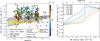Fig. 7

Evolution of the mass-metallicity gradient relation in the MW. The left panel shows the evolution of the ISM radial metallicity gradient as a function of the MW stellar mass. The vertical width of the filled area is limited by the birth metallicity gradient uncertainty (see Fig. 5). The color of the filled area corresponds to the MW stellar mass at a given epoch, which was adapted from Snaith et al. (2015). For comparison, we also provide measurements of external galaxies, the barred NIHAO-UHD galaxy (magenta line), and TNG50 (asterisks and the gray area reflect the peak value and the distribution of metallicity gradient from Hemler et al. 2021). The observational data points adapted from Queyrel et al. (2012); Simons et al. (2021); Wuyts et al. (2016); Förster Schreiber et al. (2018); Li et al. (2022); Ju et al. (2025). The right panel provides the evolution of the stellar mass-weighted radial metallicity gradient for different gradient evolution timescales, α (see Section 5.2 for more details). The analysis of the TNG50 galaxies (see Fig. C.5) and the relatively short active phase of stellar radial migration action support the rapid transformation of the mono-age stellar gradient, favoring the MW stellar metallicity gradient evolution with α = 1–2 Gyr.

5.2 Stellar metallicity gradient

Another potential application of the data obtained using the birth radii reconstruction is the possibility to explore how the total stellar metallicity gradient evolved in the MW. Since we know the birth (or ISM) and the present day gradients for mono-age populations, we need to assume how the masses of these populations and gradients evolve with time between these two points. Mass evolution can be obtained pretty straightforwardly. For each mono-age population, we adopt the initial mass from the MW star formation history (Snaith et al. 2015). Then, the mass evolution of each mono-age population is governed by the mass loss by massive stars, which we calculate using chempy (Rybizki et al. 2017)⁴ assuming a single burst model, Chabrier initial mass function (Chabrier 2003) and the contribution from SNI (Seitenzahl et al. 2013), SNII (Nomoto et al. 2013) and AGB stars (Karakas 2010). As a result, we obtained the mass evolution for mono-age populations accounting for the stellar mass loss (winds) of stars and stars dying in the SNe. We note that the high uncertainties in stellar ages, MW star formation history, and other parameters make no big difference if we choose different sets of yields and initial mass functions. Under any reasonable assumption, the stellar mass loss happens quite rapidly, yielding about 40–50% of the initial mass after 1–2 Gyr since the mono-age population formation with a negligible amount of the mass loss at later times.

The evolution of the metallicity gradient for a mono-age population with the known starting and end points is not trivial. In Figure 5, we showed that the initial (at birth) gradient is always steeper than the final one (present day) for all ages, suggesting a monotonic flattening. This aligns with the assumption about the evolution of the mono-age stellar population gradient governed by radial migration. Churning (change of the angular momentum) disk stars by spiral arms is most efficient for young populations while they are on nearly circular orbits (Sellwood & Binney 2002; Roškar et al. 2008a); once stars are heated, the probability for them to be churned decreases. Hence, we can assume that the metallicity gradient of mono-age populations also evolves on a short timescale. In our toy model, we assume that the evolution of the mono-age stellar radial metallicity gradient follows the following expression: $\begin{aligned} \nabla [F e / H] (t) = & \nabla [F e / H] (t_{b i r t h}) + (\nabla [F e / H] (t_{n o w}) \\ - \nabla [F e / H] (t_{birth})) \times Θ (t), \end{aligned}$ $\[\begin{aligned}\nabla[\mathrm{Fe} / \mathrm{H}](\mathrm{t})= & \nabla[Fe / H]\left(t_{birth}\right)+\left(\nabla[Fe/H]\left(t_{now}\right)\right. \\& \left.-\nabla[\mathrm{Fe} / \mathrm{H}]\left(\mathrm{t}_{\text {birth }}\right)\right) \times \Theta(\mathrm{t}),\end{aligned}\]$

where $Θ (t) = \frac{\erf ((t - t_{birth})) / (\sqrt{2} α))}{\erf ((0 - t_{birth})) / (\sqrt{2} α))} .$ $\[\Theta(\mathrm{t})=\frac{\left.\operatorname{erf}\left(\left(\mathrm{t}-\mathrm{t}_{\text {birth }}\right)\right) /(\sqrt{2} \alpha)\right)}{\left.\operatorname{erf}\left(\left(0-\mathrm{t}_{\text {birth }}\right)\right) /(\sqrt{2} \alpha)\right)}.\]$

These expressions parameterize the flattening of the gradient with time and are scaled by the initial and the present day values. The shape of the function is controlled by the α parameter, which indicates how rapidly the gradient transforms. The shape of the corresponding functions for α = 1 Gyr is presented in Figure C.5 (right) where the colored lines reflect different possible evolutions of stellar metallicity gradients for different mono-age populations with the starting (birth) and final (present day) points taken from Figure 5. The choice of particular parameterization does not play a significant role, as it only needs to provide a monotonic transition from initial to final gradient value with a single parameter controlling the timescale of transition.

In order to verify how reasonable the adopted model (right panel of Figure C.5) is, we present the evolution of the mono-age stellar gradient evolution in four TNG50 galaxies in our sample. As one can see, the parameterization we use agrees nicely with the mono-age metallicity gradients evolution in terms of the global shape, highlighting a rapid change on a scale of 1–2 Gyr with negligible evolution later on. The TNG50 galaxies show a number of short timescale variations and non-monotonic behavior (see also Renaud et al. 2025 for mono-age gradient evolution in VINTERGATAN); however, the global shape of the curves assures us with the choice of the model we made.

Once we have the mass of the MW mono-age stellar populations together with their individual evolution of the metallicity gradient, we can calculate the mass-weighed metallicity gradient evolution. In the right panel of Figure 7, we present the total stellar metallicity gradient evolution as a function of the MW stellar mass and redshift. The lines of different colors start and end at the same points, corresponding to the metallicity gradient of the oldest mono-age populations and the present day mass-weighted stellar metallicity gradient of $\approx - 0.02 d e x / k p c (\approx - 0.1 d e x r_{e f f}^{- 1})$ $\[\approx-0.02 ~\mathrm{dex} / \mathrm{kpc}\left(\approx-0.1 ~\mathrm{dex} ~\mathrm{r}_{\mathrm{eff}}^{-1}\right)\]$ , which is similar to the gradients found in the nearby galaxies of similar type (Sánchez-Blázquez et al. 2014; Zheng et al. 2017). The color of the lines corresponds to the choice of the α parameter (1–5 and 9 Gyr), governing how rapidly the mono-age gradient changes from the initial to the present day. The range of α values is chosen to demonstrate the full range of the possible evolution of the stellar metallicity gradient. Although, the α = 9 Gyr seems to be quite unrealistic, suggesting that the oldest stars have transformed their gradient recently, 1–2 Gyr ago. In this case, the steep gradient could be observed until z ~ 1 with the following rapid flattening, which is hard to understand if it were driven by the radial migration associated with cold stellar populations.

On the other hand, in models with the rapid mono-age gradient evolution (α = 1 or 2 Gyr), we can see quite an interesting picture. The stellar metallicity gradient flattens rapidly (z ~ 3–1, over ≈3.5 Gyr) to the present day value or even a zero gradient (α = 1). As this epoch corresponds to the end of the high-α sequence formation, we suggest that the stellar metallicity gradient was negligible by the end of the inner disk formation, which is somewhat different from the fully mixed ISM assumption during this epoch (Haywood et al. 2015, 2018), which as we discussed in the previous section may not be applicable if the MW was already rotationally supported (and thus implying a negative metallicity gradient). In any case, our model suggests the lack of the stellar metallicity gradient at z ≈ 1. The following evolution of the gradient is driven by the quiescent low-α disk formation phase; those mono-age populations, even forming on a steeper metallicity gradient, weakly affect the total stellar metallicity gradient.

For completeness, in Fig. 7 (right panel) we show the evolution of the total stellar gradient for α = 3–5 Gyr, revealing an intermediate evolution between α = 1 and α = 9 Gyr. However, as we argued above, we favor the models with lower α, which are more in line with our argumentation about the radial migration process and the gradients evolution in simulated galaxies (see Fig. C.5).

To summarize, we suggest that the present day stellar metallicity gradient was established at z ≈ 1, around the end of the inner disk, high-α formation, and it has not evolved significantly since then. The latter is the result of rather weak radial migration over this period of time (see Sect. 4.2.2), and also by a modest increase in the stellar mass spread out over a larger area of the disk.

6 Conclusions

The use of stellar birth radii is rapidly growing, allowing for a detailed view of the MW disk evolution with time that minimizes the effect of radial migration. Estimating R_birth requires knowledge of how the metallicity gradient evolves over time, which can be recovered through the scatter in [Fe/H] across age (Lu et al. 2024). However, as shown in Ratcliffe et al. (2024a), weakly barred galaxies exhibit a continual growth in the width of the star-forming region causing this method to fail, whereas strongly barred galaxies exhibit quenching in the bar region that grows with time allowing for the method to have better results. In this work, we proposed a correction to adjust for the time evolution of the width of the star-forming region, which allows for a more universal recovery of ∇[Fe/H](τ) and improves the ability to recover the metallicity gradient to within 5%. Applying our correction to the MW provides insight into its evolution, which we put into context to allow for comparisons to external galaxies. Our main conclusions are as follows:

Our proposed correction – which captures the growth of the star-forming region – is dependent on bar strength (Figure 1), and appears to be independent of simulation prescriptions for stronger-barred galaxies (left panel of Figure 4). This growth creates a non-negligible effect on the correlation between ∇[Fe/H](τ) and the scatter in [Fe/H] for different age bins. For weakly barred galaxies, ΔR(τ) can vary from galaxy to galaxy (Figures 1 and the right panel of Figure 4), but there is an overall improvement on the relationship between the metallicity range and gradient after applying our proposed correction;
In applying our proposed correction to the MW (Figures 5 and 7), we find that the ISM metallicity gradient was as steep as −0.14 dex/kpc until z ≈ 1, with a prominent non-monotonic variation at the time of the GSE infall and end of the inner high-α disk formation (≈9 Gyr ago). This is followed by a gradual flattening to ≈ −0.07 dex/kpc $(\approx - 0.35 d e x r_{eff}^{- 1})$ $\[\left(\approx-0.35 ~\mathrm{dex} ~\mathrm{r}_{\text {eff }}^{-1}\right)\]$ at present;
The birth radii distributions of young stars at different Galactic radii always peak close to the current radius location, assuring the reliability of our method (Figure 6). Using this improved method, we find that the Sun formed at 6.46 ± 0.59 kpc;
We find that the migration rate varies with age and, as expected, it is higher for older stars. However, we observe a noticeable decline in migration for stars younger than 6 Gyr showing little migration (⪅1 kpc) while the older stars migrate more than 2.5 kpc from their birthplaces. Such a sharp transition cannot be explained by the accumulated migration, as its effect saturates with time. Therefore, we suggest that different migration mechanisms dominated in different epochs of the MW evolution (such as interactions, spiral arms, bar formation);
Using assumptions regarding the mono-age stellar metallicity gradient evolution, in agreement with simulated galaxies, we introduced a model for reconstructing the total stellar metallicity gradient evolution in the MW up to redshift ≈3 (Figure 7). Relying on the arguments about the radial migration efficiency, we favor models with a rapid mono-age gradient transformation which suggest a nearly flat stellar metallicity gradient since z ≈ 1, of < −0.03 dex/kpc ( $\approx - 0.1 d e x r_{e f f}^{- 1}$ $\[\approx-0.1 ~\mathrm{dex} ~\mathrm{r}_{\mathrm{eff}}^{-1}\]$ ).

Our results illustrate that accounting for the growth of the star-forming region in a galactic disk is mandatory to accurately recover ∇[Fe/H](τ) from Range[Fe/H](age). This was also stressed in Prantzos et al. (2023), who showed the range of birth radii present in the solar neighborhood is not constant with time; the previous assumption of this method that ΔR(τ) = ΔR does not hold. Even though our correction is recovered from simulations and omits MW-specific variations in ΔR (age), we expect any deviations from Figure 5 to be small. This is because our gradient is recovered from the scatter in [Fe/H] across age using a method that captures the bulk of the star-forming region in the disk, and ignores any spurious star formation. Additionally, our recovered mono-age birth radii distributions for APOGEE DR17 red giant disk stars with ages from distmass and Anders et al. (2023) are reassuring that our correction indeed works on the MW disk, and provides better R_birth estimates. To choose the optimal steepest gradient strength, we minimize |R − R_birth| for stars with ages <2 Gyr as we expect these stars have not had the opportunity to move far away from their birth sites. However, nearly 2 Gyr old stars may have had enough time to net migrate outward (e.g., Lian et al. 2022). Therefore we acknowledge that in an ideal setting we would be minimizing the migration strength for only the extremely young stars (<0.5 Gyr or so), but due to age catalog limitations we have to minimize over this 0–2 Gyr age group. Minimizing over different criteria changed the reported steepest gradient and subsequent migration strengths, but the shape of the recovered gradient (Figure 5) and trends with migration strength (Table 1) remained in agreement. If more net outward migration is required for the 0–2 Gyr age group, then the steepest gradient would decrease to ~−0.15 dex/kpc, depending on how much migration is warranted.

The proposed correction to the range in [Fe/H] across age (Section 3.1) was applied in this work without stacking the galaxies (e.g., Cheng et al. 2024). While we find stacking does not alter our results, we choose to provide the non-stacked correction as the growth of the galactic disks are naturally already accounted for in the bar strength separation (see Khoperskov et al. 2024a).

The rapidly expanding body of research using stellar birth radii (e.g., Minchev et al. 2018; Frankel et al. 2018, 2020; Lu et al. 2024; Ratcliffe et al. 2023; Wang et al. 2024; Ratcliffe et al. 2024b; Spitoni et al. 2024; Marques et al. 2025; Plotnikova et al. 2024) offers a valuable new opportunity to explore not only radial migration within the MW disk, but also to impose tighter constraints on its historical evolution. Moreover, this research enables detailed comparisons with external galaxies up to redshift of ≈3. With the forthcoming data from large-scale Galactic spectroscopic surveys such as 4MOST (de Jong et al. 2019), WEAVE (Dalton et al. 2012), and SDSS-V (Kollmeier et al. 2017), these constraints are expected to become even more precise. This will significantly enhance our understanding of the MW evolution, as well as that of its analogs, both in the nearby universe and at higher redshifts, filling the gaps in galaxy evolution theory in general.

Acknowledgements

B.R. and I.M. acknowledge support by the Deutsche Forschungsgemeinschaft under the grant MI 2009/2-1.

Appendix A NPMLE

Each observed value (age_i, [Fe/H]_i) = Y_i can be assumed to follow $Y_{i} = Θ_{i} + ϵ_{i} ϵ_{i} \sim N_{d} (0, Σ_{i})$ $\[Y_{i}=\Theta_{i}+\epsilon_{i} \qquad \epsilon_{i} \sim N_{d}(0, \Sigma_{i})\]$

where Σ_i is the known measurement uncertainty ∀ i and Θ_i represents the true (age, [Fe/H]) value for star i. If we assume the Θ_i’s are i.i.d. from a prior distribution G and are independent with the ϵ_i’s, then the Y_i’s can be modeled as $Y_{i} ∣ Θ_{i} = θ \sim N_{d} (θ, Σ_{i}) .$ $\[Y_{i} {\mid} \Theta_{i}=\theta \sim N_{d}(\theta, \Sigma_{i}).\]$

Our main goal is to denoise our observed values Y_i, and try to recover the true Θ_i. Depending on the structure of the unknown Θ_i’s, it is possible to get significant improvements over the typically used estimator Y_i by using information from the other stellar measurements (Y_j, j ≠ i) in addition to Y_i to estimate Θ_i. An example of this could be if you have a star with an age estimate of 15 Gyr, the age estimates of the other stars (which would be < 13 Gyr) could help provide a more reliable estimate. In order to use this additional information, we used the oracle Bayes estimator: $θ_{i}^{*} = E (Θ_{i}^{*} ∣ Y_{i}) Θ^{*} \sim G Y_{i} ∣ Θ^{*} = θ \sim N_{d} (θ, Σ_{i}),$ $\[\theta_{i}^{*}=E(\Theta_{i}^{*} {\mid} Y_{i}) \qquad \Theta^{*} \sim G \qquad Y_{i} {\mid} \Theta^{*}=\theta \sim N_{d}(\theta, \Sigma_{i}),\]$

which can be rewritten as $θ_{i}^{*} = E (Θ^{*} ∣ Y_{i}) = Y_{i} + Σ_{i} \frac{\nabla f_{G, Σ_{i}} (Y_{i})}{f_{G, Σ_{i}} (Y_{i})},$ $\[\theta_{i}^{*}=E(\Theta^{*} {\mid} Y_{i})=Y_{i}+\Sigma_{i} \frac{\nabla f_{G, \Sigma_{i}}(Y_{i})}{f_{G, \Sigma_{i}}(Y_{i})},\]$

where f_{G,Σ_i}(Y_i) is the marginal density of Y_i. In order to feasibly get an estimate of $θ_{i}^{*}$ $\[\theta_{i}^{*}\]$ , we need to estimate G. The NPMLE of G is given by $\hat{G} \in \underset{G}{argmax} \prod_{i = 1}^{n} f_{G, Σ_{i}} (Y_{i}) .$ $\[\hat{G} \in \underset{G}{\operatorname{argmax}} {\prod}_{i=1}^{n} f_{G, \Sigma_{i}}(Y_{i}).\]$

After solving for $\hat{G}$ $\[\hat{G}\]$ , the denoised values can be solved as the posterior means. We refer the reader to Soloff et al. (2025) for more information.

Appendix B Scale lengths

As mentioned in Section 2, we scale each simulated galaxy to match the MW’s size; this is a common practice that allows for direct comparison between different simulated galaxies and the MW. The disk scale lengths provided by the TNG50 simulation from Sotillo-Ramos et al. (2022) are measured by fitting an exponential profile to the radial stellar surface density distribution within one to four times the half-mass radius excluding the bulge region. However, many of these galaxies are estimated to have disk scale lengths significantly too large, and in some cases some that encompass nearly the entirety of the disk (see left 2 panels of Figure B.1). This overestimation of the disk scale length causes galaxies to be too small once scaled to be comparable with the MW, meaning ΔR(τ) will be too small, especially at higher redshift. Thus we visually inspected the radial profile fit for each of the TNG50 MW/Andromeda-like galaxies to better estimate the disk scale lengths.

We calculated the disk scale lengths by fitting a linear profile to the log-scale of the radial stellar surface density distribution, excluding the bulge region and the halo, at redshift 0. The radial surface density distribution was calculated by establishing radial bins with a width of 0.5 kpc from the center of the galaxy, measured every 0.1 kpc. The bulge region and halo were identified individually for each of the galaxies by assessing the surface density, edge-on, and face-on profiles. To isolate the disk, we focused on stars born and currently located within the disk (|z| < 1 kpc, |z_birth| < 1 kpc, and born bound to the host galaxy). The right panel of Figure B.1 provides a comparison between the TNG50 disk scale lengths and ours.

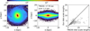Fig. B.1

Illustration of the disk scale lengths calculated in this work compared to those from Sotillo-Ramos et al. (2022). The left and middle panels show the face-on and edge-on view of a strongly barred TNG50 MW/Andromeda analog (subhalo 544001) whose disk scale length provided by TNG50 is significantly overestimated at 17.76 kpc. We estimate the disk scale length to be 5 kpc, which appears to be a better estimate. The right panel provides a comparison between the TNG50 disk scale lengths and ours. We find that the majority of galaxies have smaller disk scale lengths than found in Sotillo-Ramos et al. (2022).

Appendix C Extra figures

Figure C.1 provides the [Fe/H]–R_birth profile for 2 barred galaxies (top TNG50, bottom NIHAO-UHD) at different lookback times. In both galaxies, the gradient can be well approximated by a line.

Figure C.2 showcases the recovered metallicity gradient using different methods to calculate the scatter in [Fe/H] across different age bins. The overall shape of the recovered gradient is consistent regardless of which percentile or standard deviation is used, providing the method does not capture spurious star formation (such as the case when using the 99-1 percentiles).

Figure C.3 is a re-creation of Figure 6 in Ratcliffe et al. (2024a), using the disk scale lengths we measured for this work (see Appendix B). Here, the top panel provides the width of the star forming region in kpc, whereas Figure 1 provides the fractional difference in the width of the star forming region.

Figure C.4 demonstrates the success using the correction provided in this paper. The left panel shows the true (red line) and recovered metallicity gradients (dashed gray and black lines) in NIHAO-UHD galaxy g2.79e12 with no uncertainties added to (age, [Fe/H]). The recovered ∇[Fe/H](τ) using the method proposed in Lu et al. (2024) does a reasonable job of capturing the shape of the gradient; however, it overestimates the gradient at younger ages and underestimates at older ages. Correcting for the time variation in the width of the star-forming region (dashed black line) provides a much better recovery. The middle panel illustrates the necessity of denoising the age–metallicity relation in the presence of present day observational uncertainties. Once uncertainties are added, the recovered ∇[Fe/H](τ) is too steep at older ages, and the gradient is too smooth. The right panel shows that after denoising, the recovery is similar to when no uncertainties were added (such as in the left panel).

The left panel of Figure C.5 shows the evolution of the radial metallicity gradient in four TNG50 MW/Andromeda-like galaxies. The colored lines correspond to different mono-age populations. The right panel shows the results of how a mono-age gradient evolves over time, estimated from our Model in Section 5.

The top panel of Figure C.6 provides the age–metallicity relation for our APOGEE sample. To have the best understanding of the evolution of our Galaxy, we redraw new ages and metallicity measurements for each star before denoising to estimate the error on the recovered gradient. The bottom panel of Figure C.6 illustrates an example of the denoised age–metallicity relation.

Figure C.7 shows the ISM metallicity gradient evolution for the MW colored by the star formation rate at a given redshift. This provides an extra dimension in determining MW analogs.

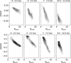Fig. C.1

Birth gradient evolution of a barred TNG50 MW-like galaxy (top panels; subhalo 577372) and the barred NIHAO-UHD galaxy (bottom panels; g2.79e12). The galaxy g2.79e12 experienced a massive merger ~9.5 Gyr and ~4 Gyr ago, and its bar formed just under 8 Gyr ago. In both galaxies, the gradient can be well approximated by a line.

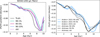Fig. C.2

Illustration of different ways to calculate the scatter in [Fe/H] when recovering the metallicity gradient in NIHAO-UHD galaxy g2.79e12 (left panel). The shape is consistent when using different percentiles to calculate the range in [Fe/H], and also consistent when using the standard deviation even when the [Fe/H] distribution is skewed at a given age. Using the 99-1 percentiles yields the worst results, as it includes too many outliers, while the other methods focus on the main star forming region. The right panel provides the MW gradient recovered using different percentiles for calculating the scatter in [Fe/H] across age bins. Each method shows multiple fluctuations in the gradient, and a birth metallicity gradient weakening with time. Figure 5 uses the standard deviation.

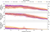Fig. C.3

Re-creation of Figure 6 from Ratcliffe et al. (2024a) using the disk scale lengths we calculated for this work. The overall trends of the growth of the star forming region per bar strength category are similar as found in that work; however, here the disks are forming stars on a larger region ~12 Gyr ago. This is due to the previously used disk scale lengths being typically too large, thus shrinking the galaxies too much when scaling to the MW (see Section B).

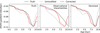Fig. C.4

Ability to recover ∇[Fe/H](τ) from Range[Fe/H](age) in g2.79e12 without any observational errors added (left panel). The middle panel is the same as the left panel but with 15% age and 0.05 dex[Fe/H] uncertainties added. The range becomes artificially high at older ages past the knee in the age–metallicity relation due to present day age errors. The recovery of ∇[Fe/H](τ) using the denoised age-metallicity relation is given in the right panel. The comparison between denoising the data and the truth (left panel) is strikingly similar.

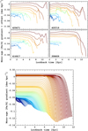Fig. C.5

Four top panels: Evolution of the radial metallicity gradient for mono-age stellar populations in four barred TNG50 galaxies. Bottom panel: Assumed evolution of the mono-abundance metallicity gradients in the MW. In all plots, the lines of different colors correspond to populations of different ages, where red represents older populations, and blue shows the evolution of younger populations. In the right panel, the initial and present day gradient values are obtained in this work and presented in Fig. 5. The mono-age metallicity gradient evolution model is described in Section. 5.2 with the timescale parameter α = 1 Gyr.

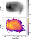Fig. C.6

Raw density distribution of the age–metallicity relation for our APOGEE disk sample with distmass ages (top panel) compared to the recovered age–metallicity relation after denoising for one of the 100 Monte Carlo samples (bottom panel).

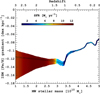Fig. C.7

Evolution of the ISM radial metallicity gradient as a function of the MW stellar mass. The vertical width of the filled area is limited by the birth metallicity gradient uncertainty, where the mean value is shown within the black lines. The color of the filled area corresponds to the star formation rate, which, together with the stellar mass growth of the MW, was adapted from Snaith et al. (2015).

References

Abdurro’uf, Accetta, K., Aerts, C., et al. 2022, ApJS, 259, 35 [NASA ADS] [CrossRef] [Google Scholar]
Agertz, O., Renaud, F., Feltzing, S., et al. 2021, MNRAS, 503, 5826 [NASA ADS] [CrossRef] [Google Scholar]
Anders, F., Gispert, P., Ratcliffe, B., et al. 2023, A&A, 678, A158 [NASA ADS] [CrossRef] [EDP Sciences] [Google Scholar]
Annem, B., & Khoperskov, S. 2024, MNRAS, 527, 2426 [Google Scholar]
Arellano-Córdova, K. Z., Esteban, C., García-Rojas, J., & Méndez-Delgado, J. E. 2021, MNRAS, 502, 225 [CrossRef] [Google Scholar]
Asplund, M., Grevesse, N., Sauval, A. J., & Scott, P. 2009, ARA&A, 47, 481 [NASA ADS] [CrossRef] [Google Scholar]
Asplund, M., Amarsi, A. M., & Grevesse, N. 2021, A&A, 653, A141 [NASA ADS] [CrossRef] [EDP Sciences] [Google Scholar]
Baba, J., Saitoh, T. R., & Tsujimoto, T. 2023, MNRAS, 526, 6088 [Google Scholar]
Belokurov, V., & Kravtsov, A. 2022, MNRAS, 514, 689 [NASA ADS] [CrossRef] [Google Scholar]
Belokurov, V., Erkal, D., Evans, N. W., Koposov, S. E., & Deason, A. J. 2018, MNRAS, 478, 611 [Google Scholar]
Belokurov, V., Sanders, J. L., Fattahi, A., et al. 2020, MNRAS, 494, 3880 [Google Scholar]
Bensby, T., Feltzing, S., & Oey, M. S. 2014, A&A, 562, A71 [NASA ADS] [CrossRef] [EDP Sciences] [Google Scholar]
Beraldo e Silva, L., Debattista, V. P., Nidever, D., Amarante, J. A. S., & Garver, B. 2021, MNRAS, 502, 260 [NASA ADS] [CrossRef] [Google Scholar]
Bland-Hawthorn, J., Krumholz, M. R., & Freeman, K. 2010, ApJ, 713, 166 [CrossRef] [Google Scholar]
Bland-Hawthorn, J., & Gerhard, O. 2016, ARA&A, 54, 529 [Google Scholar]
Blanton, M. R., Bershady, M. A., Abolfathi, B., et al. 2017, AJ, 154, 28 [Google Scholar]
Boissier, S., & Prantzos, N. 1999, MNRAS, 307, 857 [NASA ADS] [CrossRef] [Google Scholar]
Boissier, S., & Prantzos, N. 2000, MNRAS, 312, 398 [Google Scholar]
Bonanno, A., Schlattl, H., & Paternò, L. 2002, A&A, 390, 1115 [NASA ADS] [CrossRef] [EDP Sciences] [Google Scholar]
Bournaud, F., Elmegreen, B. G., & Martig, M. 2009, ApJ, 707, L1 [Google Scholar]
Bovy, J., Leung, H. W., Hunt, J. A. S., et al. 2019, MNRAS, 490, 4740 [Google Scholar]
Bresolin, F., & Kennicutt, R. C. 2015, MNRAS, 454, 3664 [CrossRef] [Google Scholar]
Brook, C. B., Kawata, D., Gibson, B. K., & Freeman, K. C. 2004, ApJ, 612, 894 [NASA ADS] [CrossRef] [Google Scholar]
Brook, C. B., Gibson, B. K., Martel, H., & Kawata, D. 2005, ApJ, 630, 298 [NASA ADS] [CrossRef] [Google Scholar]
Buck, T. 2020, MNRAS, 491, 5435 [NASA ADS] [CrossRef] [Google Scholar]
Buck, T., Ness, M. K., Macciò, A. V., Obreja, A., & Dutton, A. A. 2018, ApJ, 861, 88 [Google Scholar]
Buck, T., Macciò, A. V., Dutton, A. A., Obreja, A., & Frings, J. 2019a, MNRAS, 483, 1314 [NASA ADS] [CrossRef] [Google Scholar]
Buck, T., Ness, M., Obreja, A., Macciò, A. V., & Dutton, A. A. 2019b, ApJ, 874, 67 [NASA ADS] [CrossRef] [Google Scholar]
Buck, T., Obreja, A., Macciò, A. V., et al. 2020, MNRAS, 491, 3461 [Google Scholar]
Buck, T., Rybizki, J., Buder, S., et al. 2021, MNRAS, 508, 3365 [NASA ADS] [CrossRef] [Google Scholar]
Buck, T., Obreja, A., Ratcliffe, B., et al. 2023, MNRAS, 523, 1565 [CrossRef] [Google Scholar]
Buder, S., Sharma, S., Kos, J., et al. 2021, MNRAS, 506, 150 [NASA ADS] [CrossRef] [Google Scholar]
Buder, S., Lind, K., Ness, M. K., et al. 2022, MNRAS, 510, 2407 [NASA ADS] [CrossRef] [Google Scholar]
Buder, S., Mijnarends, L., & Buck, T. 2024, MNRAS, 532, 1010 [Google Scholar]
Buitrago, F., & Trujillo, I. 2024, A&A, 682, A110 [NASA ADS] [CrossRef] [EDP Sciences] [Google Scholar]
Byrd, R. H., Lu, P., Nocedal, J., & Zhu, C. 1995, SIAM J. Sci. Comput., 16, 1190 [Google Scholar]
Carrillo, A., Ness, M. K., Hawkins, K., et al. 2023, ApJ, 942, 35 [NASA ADS] [CrossRef] [Google Scholar]
Carrillo, A., Deason, A. J., Fattahi, A., Callingham, T. M., & Grand, R. J. J. 2024, MNRAS, 527, 2165 [Google Scholar]
Carton, D., Brinchmann, J., Contini, T., et al. 2018, MNRAS, 478, 4293 [NASA ADS] [CrossRef] [Google Scholar]
Chabrier, G. 2003, PASP, 115, 763 [Google Scholar]
Chen, T., & Prantzos, N. 2025, A&A, 694, A120 [NASA ADS] [CrossRef] [EDP Sciences] [Google Scholar]
Cheng, Y., Giavalisco, M., Simons, R. C., et al. 2024, ApJ, 964, 94 [NASA ADS] [CrossRef] [Google Scholar]
Conroy, C., Weinberg, D. H., Naidu, R. P., et al. 2022, arXiv e-prints [arXiv:2204.02989] [Google Scholar]
Cresci, G., Mannucci, F., Maiolino, R., et al. 2010, Nature, 467, 811 [Google Scholar]
Cunningham, E. C., Sanderson, R. E., Johnston, K. V., et al. 2022, ApJ, 934, 172 [NASA ADS] [CrossRef] [Google Scholar]
Dalton, G., Trager, S. C., Abrams, D. C., et al. 2012, SPIE Conf. Ser., 8446, 84460P [Google Scholar]
de Jong, R. S., Agertz, O., Berbel, A. A., et al. 2019, The Messenger, 175, 3 [NASA ADS] [Google Scholar]
Deharveng, L., Peña, M., Caplan, J., & Costero, R. 2000, MNRAS, 311, 329 [NASA ADS] [CrossRef] [Google Scholar]
Di Matteo, P., Haywood, M., Lehnert, M. D., et al. 2019, A&A, 632, A4 [NASA ADS] [CrossRef] [EDP Sciences] [Google Scholar]
Esteban, C., Fang, X., García-Rojas, J., & Toribio San Cipriano, L. 2017, MNRAS, 471, 987 [NASA ADS] [CrossRef] [Google Scholar]
Förster Schreiber, N. M., Renzini, A., Mancini, C., et al. 2018, ApJS, 238, 21 [Google Scholar]
Francois, P., & Matteucci, F. 1993, A&A, 280, 136 [Google Scholar]
Frankel, N., Rix, H.-W., Ting, Y.-S., Ness, M., & Hogg, D. W. 2018, ApJ, 865, 96 [NASA ADS] [CrossRef] [Google Scholar]
Frankel, N., Sanders, J., Rix, H.-W., Ting, Y.-S., & Ness, M. 2019, ApJ, 884, 99 [Google Scholar]
Frankel, N., Sanders, J., Ting, Y.-S., & Rix, H.-W. 2020, ApJ, 896, 15 [NASA ADS] [CrossRef] [Google Scholar]
Freeman, K., & Bland-Hawthorn, J. 2002, ARA&A, 40, 487 [Google Scholar]
García Pérez, A. E., Allende Prieto, C., Holtzman, J. A., et al. 2016, AJ, 151, 144 [Google Scholar]
Géron, T., Smethurst, R. J., Lintott, C., et al. 2024, ApJ, 973, 129 [CrossRef] [Google Scholar]
Gibson, B. K., Pilkington, K., Brook, C. B., Stinson, G. S., & Bailin, J. 2013, A&A, 554, A47 [CrossRef] [EDP Sciences] [Google Scholar]
González Delgado, R. M., García-Benito, R., Pérez, E., et al. 2015, A&A, 581, A103 [Google Scholar]
Griffith, E. J., Hogg, D. W., Hasselquist, S., et al. 2024, arXiv e-prints [arXiv:2410.22121] [Google Scholar]
Gusev, A. S., Pilyugin, L. S., Sakhibov, F., et al. 2012, MNRAS, 424, 1930 [CrossRef] [Google Scholar]
Halle, A., Di Matteo, P., Haywood, M., & Combes, F. 2015, A&A, 578, A58 [NASA ADS] [CrossRef] [EDP Sciences] [Google Scholar]
Hawkins, K. 2023, MNRAS, 525, 3318 [NASA ADS] [CrossRef] [Google Scholar]
Hayden, M. R., Bovy, J., Holtzman, J. A., et al. 2015, ApJ, 808, 132 [Google Scholar]
Haywood, M., Di Matteo, P., Lehnert, M. D., Katz, D., & Gómez, A. 2013, A&A, 560, A109 [NASA ADS] [CrossRef] [EDP Sciences] [Google Scholar]
Haywood, M., Di Matteo, P., Snaith, O., & Lehnert, M. D. 2015, A&A, 579, A5 [NASA ADS] [CrossRef] [EDP Sciences] [Google Scholar]
Haywood, M., Di Matteo, P., Lehnert, M., et al. 2018, A&A, 618, A78 [NASA ADS] [CrossRef] [EDP Sciences] [Google Scholar]
Haywood, M., Snaith, O., Lehnert, M. D., Di Matteo, P., & Khoperskov, S. 2019, A&A, 625, A105 [NASA ADS] [CrossRef] [EDP Sciences] [Google Scholar]
Haywood, M., Khoperskov, S., Cerqui, V., et al. 2024, A&A, 690, A147 [NASA ADS] [CrossRef] [EDP Sciences] [Google Scholar]
Helmi, A., Babusiaux, C., Koppelman, H. H., et al. 2018, Nature, 563, 85 [Google Scholar]
Hemler, Z. S., Torrey, P., Qi, J., et al. 2021, MNRAS, 506, 3024 [NASA ADS] [CrossRef] [Google Scholar]
Hilmi, T., Minchev, I., Buck, T., et al. 2020, MNRAS, 497, 933 [Google Scholar]
Ho, A. Y. Q., Ness, M. K., Hogg, D. W., et al. 2017a, ApJ, 836, 5 [NASA ADS] [CrossRef] [Google Scholar]
Ho, A. Y. Q., Rix, H.-W., Ness, M. K., et al. 2017b, ApJ, 841, 40 [CrossRef] [Google Scholar]
Holtzman, J. A., Shetrone, M., Johnson, J. A., et al. 2015, AJ, 150, 148 [Google Scholar]
Horta, D., Schiavon, R. P., Mackereth, J. T., et al. 2023, MNRAS, 520, 5671 [NASA ADS] [CrossRef] [Google Scholar]
Hou, J. L., Prantzos, N., & Boissier, S. 2000, A&A, 362, 921 [NASA ADS] [Google Scholar]
Ibata, R. A., Gilmore, G., & Irwin, M. J. 1994, Nature, 370, 194 [Google Scholar]
Imig, J., Price, C., Holtzman, J. A., et al. 2023, ApJ, 954, 124 [CrossRef] [Google Scholar]
Jones, T., Ellis, R. S., Richard, J., & Jullo, E. 2013, ApJ, 765, 48 [NASA ADS] [CrossRef] [Google Scholar]
Jones, T., Wang, X., Schmidt, K. B., et al. 2015, AJ, 149, 107 [NASA ADS] [CrossRef] [Google Scholar]
Jönsson, H., Holtzman, J. A., Allende Prieto, C., et al. 2020, AJ, 160, 120 [Google Scholar]
Ju, M., Wang, X., Jones, T., et al. 2025, ApJ, 978, L39 [Google Scholar]
Karakas, A. I. 2010, MNRAS, 403, 1413 [NASA ADS] [CrossRef] [Google Scholar]
Khoperskov, S., Haywood, M., Di Matteo, P., Lehnert, M. D., & Combes, F. 2018, A&A, 609, A60 [NASA ADS] [CrossRef] [EDP Sciences] [Google Scholar]
Khoperskov, S., Di Matteo, P., Haywood, M., Gómez, A., & Snaith, O. N. 2020, A&A, 638, A144 [NASA ADS] [CrossRef] [EDP Sciences] [Google Scholar]
Khoperskov, S., Haywood, M., Snaith, O., et al. 2021, MNRAS, 501, 5176 [NASA ADS] [CrossRef] [Google Scholar]
Khoperskov, S., Minchev, I., Libeskind, N., et al. 2023a, A&A, 677, A91 [NASA ADS] [CrossRef] [EDP Sciences] [Google Scholar]
Khoperskov, S., Minchev, I., Steinmetz, M., et al. 2023b, arXiv e-prints [arXiv:2310.05287] [Google Scholar]
Khoperskov, S., Minchev, I., Steinmetz, M., et al. 2024a, MNRAS, 533, 3975 [CrossRef] [Google Scholar]
Khoperskov, S., Steinmetz, M., Haywood, M., et al. 2024b, A&A, submitted [arXiv:2411.16866] [Google Scholar]
Kollmeier, J. A., Zasowski, G., Rix, H.-W., et al. 2017, arXiv e-prints [arXiv:1711.03234] [Google Scholar]
Kordopatis, G., Binney, J., Gilmore, G., et al. 2015, MNRAS, 447, 3526 [Google Scholar]
Kubryk, M., Prantzos, N., & Athanassoula, E. 2013, MNRAS, 436, 1479 [NASA ADS] [CrossRef] [Google Scholar]
Kubryk, M., Prantzos, N., & Athanassoula, E. 2015, A&A, 580, A126 [NASA ADS] [CrossRef] [EDP Sciences] [Google Scholar]
Law, D. R., & Majewski, S. R. 2010, ApJ, 714, 229 [Google Scholar]
Leethochawalit, N., Jones, T. A., Ellis, R. S., et al. 2016, ApJ, 820, 84 [NASA ADS] [CrossRef] [Google Scholar]
Leung, H. W., & Bovy, J. 2019, MNRAS, 489, 2079 [CrossRef] [Google Scholar]
Li, Z., Wang, X., Cai, Z., et al. 2022, ApJ, 929, L8 [NASA ADS] [CrossRef] [Google Scholar]
Lian, J., Zasowski, G., Hasselquist, S., et al. 2022, MNRAS, 511, 5639 [NASA ADS] [CrossRef] [Google Scholar]
Lu, Y., Buck, T., Minchev, I., & Ness, M. K. 2022, MNRAS, 515, L34 [NASA ADS] [CrossRef] [Google Scholar]
Lu, Y. L., Minchev, I., Buck, T., et al. 2024, MNRAS, 535, 392 [NASA ADS] [CrossRef] [Google Scholar]
Ma, X., Hopkins, P. F., Feldmann, R., et al. 2017, MNRAS, 466, 4780 [Google Scholar]
Mackereth, J. T., & Bovy, J. 2018, PASP, 130, 114501 [Google Scholar]
Majewski, S. R., Schiavon, R. P., Frinchaboy, P. M., et al. 2017, AJ, 154, 94 [NASA ADS] [CrossRef] [Google Scholar]
Marinacci, F., Vogelsberger, M., Pakmor, R., et al. 2018, MNRAS, 480, 5113 [NASA ADS] [Google Scholar]
Marques, L., Minchev, I., Ratcliffe, B., et al. 2025, A&A, submitted [arXiv:2502.02651] [Google Scholar]
Matteucci, F. 2012, Chemical Evolution of Galaxies (Springer Science & Business Media) [CrossRef] [Google Scholar]
Minchev, I., & Famaey, B. 2010, ApJ, 722, 112 [Google Scholar]
Minchev, I., & Quillen, A. C. 2006, MNRAS, 368, 623 [NASA ADS] [CrossRef] [Google Scholar]
Minchev, I., Famaey, B., Combes, F., et al. 2011, A&A, 527, A147 [NASA ADS] [CrossRef] [EDP Sciences] [Google Scholar]
Minchev, I., Famaey, B., Quillen, A. C., et al. 2012, A&A, 548, A127 [NASA ADS] [CrossRef] [EDP Sciences] [Google Scholar]
Minchev, I., Chiappini, C., & Martig, M. 2013, A&A, 558, A9 [CrossRef] [EDP Sciences] [Google Scholar]
Minchev, I., Chiappini, C., & Martig, M. 2014, A&A, 572, A92 [CrossRef] [EDP Sciences] [Google Scholar]
Minchev, I., Anders, F., Recio-Blanco, A., et al. 2018, MNRAS, 481, 1645 [NASA ADS] [CrossRef] [Google Scholar]
Mollá, M., Ferrini, F., & Díaz, A. I. 1997, ApJ, 475, 519 [Google Scholar]
Mollá, M., Díaz, Á. I., Cavichia, O., et al. 2019, MNRAS, 482, 3071 [NASA ADS] [Google Scholar]
Moustakas, J., Kennicutt, Robert C., J., Tremonti, C. A., et al. 2010, ApJS, 190, 233 [NASA ADS] [CrossRef] [Google Scholar]
Naiman, J. P., Pillepich, A., Springel, V., et al. 2018, MNRAS, 477, 1206 [Google Scholar]
Nelson, D., Pillepich, A., Springel, V., et al. 2018, MNRAS, 475, 624 [Google Scholar]
Nelson, D., Pillepich, A., Springel, V., et al. 2019a, MNRAS, 490, 3234 [Google Scholar]
Nelson, D., Springel, V., Pillepich, A., et al. 2019b, Computat. Astrophys. Cosmol., 6, 2 [NASA ADS] [CrossRef] [Google Scholar]
Ness, M. K., Johnston, K. V., Blancato, K., et al. 2019, ApJ, 883, 177 [CrossRef] [Google Scholar]
Ness, M. K., Wheeler, A. J., McKinnon, K., et al. 2022, ApJ, 926, 144 [NASA ADS] [CrossRef] [Google Scholar]
Nieva, M. F., & Przybilla, N. 2012, A&A, 539, A143 [NASA ADS] [CrossRef] [EDP Sciences] [Google Scholar]
Nomoto, K., Kobayashi, C., & Tominaga, N. 2013, ARA&A, 51, 457 [CrossRef] [Google Scholar]
Obreja, A., Buck, T., & Macciò, A. V. 2022, A&A, 657, A15 [NASA ADS] [CrossRef] [EDP Sciences] [Google Scholar]
Pilkington, K., Few, C. G., Gibson, B. K., et al. 2012a, A&A, 540, A56 [NASA ADS] [CrossRef] [EDP Sciences] [Google Scholar]
Pilkington, K., Gibson, B. K., Brook, C. B., et al. 2012b, MNRAS, 425, 969 [Google Scholar]
Pillepich, A., Nelson, D., Hernquist, L., et al. 2018, MNRAS, 475, 648 [Google Scholar]
Pillepich, A., Nelson, D., Springel, V., et al. 2019, MNRAS, 490, 3196 [Google Scholar]
Pillepich, A., Sotillo-Ramos, D., Ramesh, R., et al. 2024, MNRAS, 535, 1721 [NASA ADS] [CrossRef] [Google Scholar]
Pilyugin, L. S., & Thuan, T. X. 2007, ApJ, 669, 299 [Google Scholar]
Pilyugin, L. S., Vílchez, J. M., & Contini, T. 2004, A&A, 425, 849 [NASA ADS] [CrossRef] [EDP Sciences] [Google Scholar]
Pilyugin, L. S., Thuan, T. X., & Vílchez, J. M. 2006, MNRAS, 367, 1139 [NASA ADS] [CrossRef] [Google Scholar]
Pilyugin, L. S., Grebel, E. K., & Kniazev, A. Y. 2014, AJ, 147, 131 [NASA ADS] [CrossRef] [Google Scholar]
Plotnikova, A., Spina, L., Ratcliffe, B., Casali, G., & Carraro, G. 2024, A&A, 691, A298 [NASA ADS] [CrossRef] [EDP Sciences] [Google Scholar]
Portinari, L., Chiosi, C., & Bressan, A. 1998, A&A, 334, 505 [NASA ADS] [Google Scholar]
Prantzos, N., Abia, C., Chen, T., et al. 2023, MNRAS, 523, 2126 [NASA ADS] [CrossRef] [Google Scholar]
Queiroz, A. B. A., Anders, F., Chiappini, C., et al. 2023, A&A, 673, A155 [NASA ADS] [CrossRef] [EDP Sciences] [Google Scholar]
Queyrel, J., Contini, T., Kissler-Patig, M., et al. 2012, A&A, 539, A93 [NASA ADS] [CrossRef] [EDP Sciences] [Google Scholar]
Ratcliffe, B. L., & Ness, M. K. 2023, ApJ, 943, 92 [Google Scholar]
Ratcliffe, B. L., Ness, M. K., Johnston, K. V., & Sen, B. 2020, ApJ, 900, 165 [Google Scholar]
Ratcliffe, B. L., Ness, M. K., Buck, T., et al. 2022, ApJ, 924, 60 [NASA ADS] [CrossRef] [Google Scholar]
Ratcliffe, B., Minchev, I., Anders, F., et al. 2023, MNRAS, 525, 2208 [NASA ADS] [CrossRef] [Google Scholar]
Ratcliffe, B., Khoperskov, S., Minchev, I., et al. 2024a, A&A, 690, A352 [NASA ADS] [CrossRef] [EDP Sciences] [Google Scholar]
Ratcliffe, B., Minchev, I., Cescutti, G., et al. 2024b, MNRAS, 528, 3464 [NASA ADS] [CrossRef] [Google Scholar]
Renaud, F., Agertz, O., Andersson, E. P., et al. 2021a, MNRAS, 503, 5868 [NASA ADS] [CrossRef] [Google Scholar]
Renaud, F., Agertz, O., Read, J. I., et al. 2021b, MNRAS, 503, 5846 [NASA ADS] [CrossRef] [Google Scholar]
Renaud, F., Ratcliffe, B., Minchev, I., et al. 2025, A&A, 694, A56 [NASA ADS] [CrossRef] [EDP Sciences] [Google Scholar]
Renu, D., Subramanian, S., Rao, S., & George, K. 2025, A&A, 696, A118 [NASA ADS] [CrossRef] [EDP Sciences] [Google Scholar]
Rix, H.-W., Chandra, V., Zasowski, G., et al. 2024, ApJ, 975, 293 [NASA ADS] [CrossRef] [Google Scholar]
Roškar, R., Debattista, V. P., Quinn, T. R., Stinson, G. S., & Wadsley, J. 2008a, ApJ, 684, L79 [Google Scholar]
Roškar, R., Debattista, V. P., Stinson, G. S., et al. 2008b, ApJ, 675, L65 [Google Scholar]
Rybizki, J., Just, A., & Rix, H.-W. 2017, A&A, 605, A59 [NASA ADS] [CrossRef] [EDP Sciences] [Google Scholar]
Ryder, S. D. 1995, ApJ, 444, 610 [NASA ADS] [CrossRef] [Google Scholar]
Sánchez, S. F., Rosales-Ortega, F. F., Jungwiert, B., et al. 2013, A&A, 554, A58 [NASA ADS] [CrossRef] [EDP Sciences] [Google Scholar]
Sánchez, S. F., Rosales-Ortega, F. F., Iglesias-Páramo, J., et al. 2014, A&A, 563, A49 [CrossRef] [EDP Sciences] [Google Scholar]
Sánchez-Blázquez, P., Rosales-Ortega, F. F., Méndez-Abreu, J., et al. 2014, A&A, 570, A6 [NASA ADS] [CrossRef] [EDP Sciences] [Google Scholar]
Sanders, J. L., Kawata, D., Matsunaga, N., et al. 2024, MNRAS, 530, 2972 [NASA ADS] [CrossRef] [Google Scholar]
Schönrich, R., & Binney, J. 2009, MNRAS, 399, 1145 [Google Scholar]
Segovia Otero, Á., Renaud, F., & Agertz, O. 2022, MNRAS, 516, 2272 [NASA ADS] [CrossRef] [Google Scholar]
Seitenzahl, I. R., Ciaraldi-Schoolmann, F., Röpke, F. K., et al. 2013, MNRAS, 429, 1156 [NASA ADS] [CrossRef] [Google Scholar]
Sellwood, J. A., & Binney, J. J. 2002, MNRAS, 336, 785 [Google Scholar]
Semenov, V. A., Conroy, C., Chandra, V., Hernquist, L., & Nelson, D. 2024a, ApJ, 962, 84 [NASA ADS] [CrossRef] [Google Scholar]
Semenov, V. A., Conroy, C., Smith, A., Puchwein, E., & Hernquist, L. 2024b, arXiv e-prints [arXiv:2409.18173] [Google Scholar]
Sharma, S., Hayden, M. R., Bland-Hawthorn, J., et al. 2022, MNRAS, 510, 734 [Google Scholar]
Simons, R. C., Papovich, C., Momcheva, I., et al. 2021, ApJ, 923, 203 [NASA ADS] [CrossRef] [Google Scholar]
Snaith, O., Haywood, M., Di Matteo, P., et al. 2015, A&A, 578, A87 [NASA ADS] [CrossRef] [EDP Sciences] [Google Scholar]
Soloff, J. A., Guntuboyina, A., & Sen, B. 2025, J. Roy. Statist. Soc. Ser. B: Statist. Methodol., 87, 1 [Google Scholar]
Sotillo-Ramos, D., Pillepich, A., Donnari, M., et al. 2022, MNRAS, 516, 5404 [NASA ADS] [CrossRef] [Google Scholar]
Spitoni, E., Matteucci, F., Gratton, R., et al. 2024, A&A, 690, A208 [NASA ADS] [CrossRef] [EDP Sciences] [Google Scholar]
Springel, V. 2010, MNRAS, 401, 791 [Google Scholar]
Springel, V., Pakmor, R., Pillepich, A., et al. 2018, MNRAS, 475, 676 [Google Scholar]
Stone-Martinez, A., Holtzman, J. A., Imig, J., et al. 2024, AJ, 167, 73 [NASA ADS] [CrossRef] [Google Scholar]
Stott, J. P., Sobral, D., Swinbank, A. M., et al. 2014, MNRAS, 443, 2695 [NASA ADS] [CrossRef] [Google Scholar]
Trentin, E., Catanzaro, G., Ripepi, V., et al. 2024, A&A, 690, A246 [NASA ADS] [CrossRef] [EDP Sciences] [Google Scholar]
van Zee, L., Salzer, J. J., Haynes, M. P., O’Donoghue, A. A., & Balonek, T. J. 1998, AJ, 116, 2805 [CrossRef] [Google Scholar]
Venturi, G., Carniani, S., Parlanti, E., et al. 2024, A&A, 691, A19 [NASA ADS] [CrossRef] [EDP Sciences] [Google Scholar]
Vila-Costas, M. B., & Edmunds, M. G. 1992, MNRAS, 259, 121 [NASA ADS] [CrossRef] [Google Scholar]
Vincenzo, F., & Kobayashi, C. 2018, MNRAS, 478, 155 [NASA ADS] [CrossRef] [Google Scholar]
Vislosky, E., Minchev, I., Khoperskov, S., et al. 2024, MNRAS, 528, 3576 [NASA ADS] [CrossRef] [Google Scholar]
Wadsley, J. W., Keller, B. W., & Quinn, T. R. 2017, MNRAS, 471, 2357 [NASA ADS] [CrossRef] [Google Scholar]
Wang, K., Carrillo, A., Ness, M. K., & Buck, T. 2024, MNRAS, 527, 321 [Google Scholar]
Wielen, R., Fuchs, B., & Dettbarn, C. 1996, A&A, 314, 438 [NASA ADS] [Google Scholar]
Wozniak, H. 2020, ApJ, 889, 81 [NASA ADS] [CrossRef] [Google Scholar]
Wuyts, E., Wisnioski, E., Fossati, M., et al. 2016, ApJ, 827, 74 [NASA ADS] [CrossRef] [Google Scholar]
Xiang, M., & Rix, H.-W. 2022, Nature, 603, 599 [NASA ADS] [CrossRef] [Google Scholar]
Zaritsky, D., Kennicutt, Robert C., J., & Huchra, J. P. 1994, ApJ, 420, 87 [NASA ADS] [CrossRef] [Google Scholar]
Zheng, Z., Wang, H., Ge, J., et al. 2017, MNRAS, 465, 4572 [Google Scholar]

¹

https://www.tng-project.org/data/milkyway+andromeda/

²

https://github.com/jake-soloff/NPEB/tree/master

³

The distmass catalog provides age errors in terms of log₁₀ yr.

⁴

https://github.com/jan-rybizki/Chempy

All Tables

Table 1

Median migration distance for stars of different ages and guiding radii.

In the text

All Figures

Fig. 1

Illustration of how the median width of the star-forming region (and 25–75 percentile shaded region) in galaxies grows with cosmic time as a function of the present day bar strength using TNG50 MW/M31-like galaxies. Each line provides the fractional difference in the width of the star forming region, relative to a lookback time of 12 Gyr. In weaker-barred galaxies, where the width of the star-forming region increases by a factor of 10, the method of recovering the metallicity gradient from the range in [Fe/H] across age bins fails. When the width of the star-forming region does not change significantly over time (such as in the strongest barred galaxies), the method produces a smaller error. For the kilo-parsec values, we refer the reader to Figure C.3.

In the text

Fig. 2

Role of denoising the age–metallicity relation in recovering the metallicity gradient from the scatter in [Fe/H] as a function of age. The age–metallicity relation for g2.79e12 (gray scale) with 15% age and 0.05 dex [Fe/H] uncertainty added (blue scale) is shown in the top panel. The horizontal lines correspond to the upper and lower bounds used to calculate Range [Fe/H] (age) measured with (blue) and without (white) measurement uncertainties. The range measured using the data with uncertainties is much larger than the range measured using the true age and [Fe/H] values for age >9 Gyr. The middle panel shows the distribution of the denoised ages (Section 3.2) and [Fe/H] (plasma) match well the age–metallicity relation of the true distribution. The presence of present day observational uncertainties (also shown in the bottom panel) makes denoising the age–metallicity relation a requirement to recover the structure in this plane, and thus Range [Fe/H] (age).

In the text

Fig. 3

Correlation between the shape of the metallicity gradient over time and the range in [Fe/H] measured across age bins using the method with (solid lines) and without (dashed lines) our proposed correction applied for our sample of 178 TNG50 MW/M31-like galaxies. The colored lines correspond to the correlation of galaxies with different bar strengths, with the black line providing the density of the entire sample. A correlation of −1 implies that the shape of the gradient can be perfectly recovered from Range[Fe/H](age), and that the method is successful. With no correction applied, the median correlation is −0.74 (median absolute percent error of 28%), whereas when applying the correction the median correlation improves to −0.88 (median absolute percent error of 20%). The correction has a smaller improvement on stronger-barred galaxies (yellow) where the method already exhibited good success, but the correlation of galaxies with weaker present day bars show an improvement of over 40%.

In the text

Fig. 4

Demonstration of how the recovered [Fe/H] gradient using our proposed correction works in g2.79e12 (left; strong bar) and g8.26e11 (right; no bar) from the NIHAO-UHD simulation suite, which are completely independent of the TNG50 galaxies that are used to determine the correction. As discussed in Section 4.1.2, we added 0.05 dex and a 15% error to [Fe/H] and age and then denoised to make the best extensions to the MW. The black line in each panel represents the recovered metallicity gradient with the correction applied, and it matches the true [Fe/H] gradient evolution of disk stars (red line) better than recovering the metallicity gradient without the correction (gray line).

In the text

Fig. 5

Comparing the recovered MW disk metallicity gradients with and without correcting for the growth of the star-forming region. The dashed gray line represents the gradient found in Ratcliffe et al. (2023) using ages from Anders et al. (2023), while ∇[Fe/H](τ) recovered using the correction proposed in this paper is shown in blue (ages from Anders et al. 2023) and gray (ages from distmass). The gradient is taken as the mean of 100 Monte Carlo samples where (age, [Fe/H]) are redrawn from a normal distribution and then denoised, and the shaded areas represent the 25–75 percentiles. The range in [Fe/H] is measured in age bin widths of 1 Gyr, taken every 0.2 Gyr. The corrected gradient recovered using the two different age catalogs is strikingly consistent and illustrates that the fluctuations in the gradient are not artifacts of the age catalog. The steepening events in the gradient ~8, ~6, and ~3 Gyr ago are less significant after the correction is applied; however, there is still non-monotonicity in the gradient’s evolution. We also provide the present day gradient (dashed purple line measured using R_guide) to illustrate the information lost due to radial migration.

In the text

Fig. 6

Birth radii distributions of the mono-age MW disk stars currently located within 0.25 dex of different radii (as indicated by the dashed black line in each panel) with |z| ≤ 0.5 kpc. The area under each mono-age curve is normalized to 1, so the curves are not representative of the relative proportion of each age at a given radii, but rather to illustrate the individual trends of each mono-age population. For each radial bin, the youngest population peaks within 0.5 kpc from where they are currently located today while each older population has consecutively smaller and smaller birth radii. Comparing the distribution of stars in the solar neighborhood (bottom left panel) to that of Ratcliffe et al. (2023), the correction used in this paper provides less migration for the 2–6 Gyr old populations and less spread in the oldest population.

In the text

Fig. 7

Evolution of the mass-metallicity gradient relation in the MW. The left panel shows the evolution of the ISM radial metallicity gradient as a function of the MW stellar mass. The vertical width of the filled area is limited by the birth metallicity gradient uncertainty (see Fig. 5). The color of the filled area corresponds to the MW stellar mass at a given epoch, which was adapted from Snaith et al. (2015). For comparison, we also provide measurements of external galaxies, the barred NIHAO-UHD galaxy (magenta line), and TNG50 (asterisks and the gray area reflect the peak value and the distribution of metallicity gradient from Hemler et al. 2021). The observational data points adapted from Queyrel et al. (2012); Simons et al. (2021); Wuyts et al. (2016); Förster Schreiber et al. (2018); Li et al. (2022); Ju et al. (2025). The right panel provides the evolution of the stellar mass-weighted radial metallicity gradient for different gradient evolution timescales, α (see Section 5.2 for more details). The analysis of the TNG50 galaxies (see Fig. C.5) and the relatively short active phase of stellar radial migration action support the rapid transformation of the mono-age stellar gradient, favoring the MW stellar metallicity gradient evolution with α = 1–2 Gyr.

In the text

Fig. B.1

Illustration of the disk scale lengths calculated in this work compared to those from Sotillo-Ramos et al. (2022). The left and middle panels show the face-on and edge-on view of a strongly barred TNG50 MW/Andromeda analog (subhalo 544001) whose disk scale length provided by TNG50 is significantly overestimated at 17.76 kpc. We estimate the disk scale length to be 5 kpc, which appears to be a better estimate. The right panel provides a comparison between the TNG50 disk scale lengths and ours. We find that the majority of galaxies have smaller disk scale lengths than found in Sotillo-Ramos et al. (2022).

In the text

	Fig. C.1 Birth gradient evolution of a barred TNG50 MW-like galaxy (top panels; subhalo 577372) and the barred NIHAO-UHD galaxy (bottom panels; g2.79e12). The galaxy g2.79e12 experienced a massive merger ~9.5 Gyr and ~4 Gyr ago, and its bar formed just under 8 Gyr ago. In both galaxies, the gradient can be well approximated by a line.
In the text

Fig. C.2

Illustration of different ways to calculate the scatter in [Fe/H] when recovering the metallicity gradient in NIHAO-UHD galaxy g2.79e12 (left panel). The shape is consistent when using different percentiles to calculate the range in [Fe/H], and also consistent when using the standard deviation even when the [Fe/H] distribution is skewed at a given age. Using the 99-1 percentiles yields the worst results, as it includes too many outliers, while the other methods focus on the main star forming region. The right panel provides the MW gradient recovered using different percentiles for calculating the scatter in [Fe/H] across age bins. Each method shows multiple fluctuations in the gradient, and a birth metallicity gradient weakening with time. Figure 5 uses the standard deviation.

In the text

Fig. C.3

Re-creation of Figure 6 from Ratcliffe et al. (2024a) using the disk scale lengths we calculated for this work. The overall trends of the growth of the star forming region per bar strength category are similar as found in that work; however, here the disks are forming stars on a larger region ~12 Gyr ago. This is due to the previously used disk scale lengths being typically too large, thus shrinking the galaxies too much when scaling to the MW (see Section B).

In the text

Fig. C.4

Ability to recover ∇[Fe/H](τ) from Range[Fe/H](age) in g2.79e12 without any observational errors added (left panel). The middle panel is the same as the left panel but with 15% age and 0.05 dex[Fe/H] uncertainties added. The range becomes artificially high at older ages past the knee in the age–metallicity relation due to present day age errors. The recovery of ∇[Fe/H](τ) using the denoised age-metallicity relation is given in the right panel. The comparison between denoising the data and the truth (left panel) is strikingly similar.

In the text

Fig. C.5

Four top panels: Evolution of the radial metallicity gradient for mono-age stellar populations in four barred TNG50 galaxies. Bottom panel: Assumed evolution of the mono-abundance metallicity gradients in the MW. In all plots, the lines of different colors correspond to populations of different ages, where red represents older populations, and blue shows the evolution of younger populations. In the right panel, the initial and present day gradient values are obtained in this work and presented in Fig. 5. The mono-age metallicity gradient evolution model is described in Section. 5.2 with the timescale parameter α = 1 Gyr.

In the text

	Fig. C.6 Raw density distribution of the age–metallicity relation for our APOGEE disk sample with `distmass` ages (top panel) compared to the recovered age–metallicity relation after denoising for one of the 100 Monte Carlo samples (bottom panel).
In the text

Fig. C.7

Evolution of the ISM radial metallicity gradient as a function of the MW stellar mass. The vertical width of the filled area is limited by the birth metallicity gradient uncertainty, where the mean value is shown within the black lines. The color of the filled area corresponds to the star formation rate, which, together with the stellar mass growth of the MW, was adapted from Snaith et al. (2015).

In the text

Current usage metrics show cumulative count of Article Views (full-text article views including HTML views, PDF and ePub downloads, according to the available data) and Abstracts Views on Vision4Press platform.

Data correspond to usage on the plateform after 2015. The current usage metrics is available 48-96 hours after online publication and is updated daily on week days.

Initial download of the metrics may take a while.

[1] Abdurro’uf, Accetta, K., Aerts, C., et al. 2022, ApJS, 259, 35 [NASA ADS] [CrossRef] [Google Scholar]

[2] Agertz, O., Renaud, F., Feltzing, S., et al. 2021, MNRAS, 503, 5826 [NASA ADS] [CrossRef] [Google Scholar]

[3] Anders, F., Gispert, P., Ratcliffe, B., et al. 2023, A&A, 678, A158 [NASA ADS] [CrossRef] [EDP Sciences] [Google Scholar]

[4] Annem, B., & Khoperskov, S. 2024, MNRAS, 527, 2426 [Google Scholar]

[5] Arellano-Córdova, K. Z., Esteban, C., García-Rojas, J., & Méndez-Delgado, J. E. 2021, MNRAS, 502, 225 [CrossRef] [Google Scholar]

[6] Asplund, M., Grevesse, N., Sauval, A. J., & Scott, P. 2009, ARA&A, 47, 481 [NASA ADS] [CrossRef] [Google Scholar]

[7] Asplund, M., Amarsi, A. M., & Grevesse, N. 2021, A&A, 653, A141 [NASA ADS] [CrossRef] [EDP Sciences] [Google Scholar]

[8] Baba, J., Saitoh, T. R., & Tsujimoto, T. 2023, MNRAS, 526, 6088 [Google Scholar]

[9] Belokurov, V., & Kravtsov, A. 2022, MNRAS, 514, 689 [NASA ADS] [CrossRef] [Google Scholar]

[10] Belokurov, V., Erkal, D., Evans, N. W., Koposov, S. E., & Deason, A. J. 2018, MNRAS, 478, 611 [Google Scholar]

[11] Belokurov, V., Sanders, J. L., Fattahi, A., et al. 2020, MNRAS, 494, 3880 [Google Scholar]

[12] Bensby, T., Feltzing, S., & Oey, M. S. 2014, A&A, 562, A71 [NASA ADS] [CrossRef] [EDP Sciences] [Google Scholar]

[13] Beraldo e Silva, L., Debattista, V. P., Nidever, D., Amarante, J. A. S., & Garver, B. 2021, MNRAS, 502, 260 [NASA ADS] [CrossRef] [Google Scholar]

[14] Bland-Hawthorn, J., Krumholz, M. R., & Freeman, K. 2010, ApJ, 713, 166 [CrossRef] [Google Scholar]

[15] Bland-Hawthorn, J., & Gerhard, O. 2016, ARA&A, 54, 529 [Google Scholar]

[16] Blanton, M. R., Bershady, M. A., Abolfathi, B., et al. 2017, AJ, 154, 28 [Google Scholar]

[17] Boissier, S., & Prantzos, N. 1999, MNRAS, 307, 857 [NASA ADS] [CrossRef] [Google Scholar]

[18] Boissier, S., & Prantzos, N. 2000, MNRAS, 312, 398 [Google Scholar]

[19] Bonanno, A., Schlattl, H., & Paternò, L. 2002, A&A, 390, 1115 [NASA ADS] [CrossRef] [EDP Sciences] [Google Scholar]

[20] Bournaud, F., Elmegreen, B. G., & Martig, M. 2009, ApJ, 707, L1 [Google Scholar]

[21] Bovy, J., Leung, H. W., Hunt, J. A. S., et al. 2019, MNRAS, 490, 4740 [Google Scholar]

[22] Bresolin, F., & Kennicutt, R. C. 2015, MNRAS, 454, 3664 [CrossRef] [Google Scholar]

[23] Brook, C. B., Kawata, D., Gibson, B. K., & Freeman, K. C. 2004, ApJ, 612, 894 [NASA ADS] [CrossRef] [Google Scholar]

[24] Brook, C. B., Gibson, B. K., Martel, H., & Kawata, D. 2005, ApJ, 630, 298 [NASA ADS] [CrossRef] [Google Scholar]

[25] Buck, T. 2020, MNRAS, 491, 5435 [NASA ADS] [CrossRef] [Google Scholar]

[26] Buck, T., Ness, M. K., Macciò, A. V., Obreja, A., & Dutton, A. A. 2018, ApJ, 861, 88 [Google Scholar]

[27] Buck, T., Macciò, A. V., Dutton, A. A., Obreja, A., & Frings, J. 2019a, MNRAS, 483, 1314 [NASA ADS] [CrossRef] [Google Scholar]

[28] Buck, T., Ness, M., Obreja, A., Macciò, A. V., & Dutton, A. A. 2019b, ApJ, 874, 67 [NASA ADS] [CrossRef] [Google Scholar]

[29] Buck, T., Obreja, A., Macciò, A. V., et al. 2020, MNRAS, 491, 3461 [Google Scholar]

[30] Buck, T., Rybizki, J., Buder, S., et al. 2021, MNRAS, 508, 3365 [NASA ADS] [CrossRef] [Google Scholar]

[31] Buck, T., Obreja, A., Ratcliffe, B., et al. 2023, MNRAS, 523, 1565 [CrossRef] [Google Scholar]

[32] Buder, S., Sharma, S., Kos, J., et al. 2021, MNRAS, 506, 150 [NASA ADS] [CrossRef] [Google Scholar]

[33] Buder, S., Lind, K., Ness, M. K., et al. 2022, MNRAS, 510, 2407 [NASA ADS] [CrossRef] [Google Scholar]

[34] Buder, S., Mijnarends, L., & Buck, T. 2024, MNRAS, 532, 1010 [Google Scholar]

[35] Buitrago, F., & Trujillo, I. 2024, A&A, 682, A110 [NASA ADS] [CrossRef] [EDP Sciences] [Google Scholar]

[36] Byrd, R. H., Lu, P., Nocedal, J., & Zhu, C. 1995, SIAM J. Sci. Comput., 16, 1190 [Google Scholar]

[37] Carrillo, A., Ness, M. K., Hawkins, K., et al. 2023, ApJ, 942, 35 [NASA ADS] [CrossRef] [Google Scholar]

[38] Carrillo, A., Deason, A. J., Fattahi, A., Callingham, T. M., & Grand, R. J. J. 2024, MNRAS, 527, 2165 [Google Scholar]

[39] Carton, D., Brinchmann, J., Contini, T., et al. 2018, MNRAS, 478, 4293 [NASA ADS] [CrossRef] [Google Scholar]

[40] Chabrier, G. 2003, PASP, 115, 763 [Google Scholar]

[41] Chen, T., & Prantzos, N. 2025, A&A, 694, A120 [NASA ADS] [CrossRef] [EDP Sciences] [Google Scholar]

[42] Cheng, Y., Giavalisco, M., Simons, R. C., et al. 2024, ApJ, 964, 94 [NASA ADS] [CrossRef] [Google Scholar]

[43] Conroy, C., Weinberg, D. H., Naidu, R. P., et al. 2022, arXiv e-prints [arXiv:2204.02989] [Google Scholar]

[44] Cresci, G., Mannucci, F., Maiolino, R., et al. 2010, Nature, 467, 811 [Google Scholar]

[45] Cunningham, E. C., Sanderson, R. E., Johnston, K. V., et al. 2022, ApJ, 934, 172 [NASA ADS] [CrossRef] [Google Scholar]

[46] Dalton, G., Trager, S. C., Abrams, D. C., et al. 2012, SPIE Conf. Ser., 8446, 84460P [Google Scholar]

[47] de Jong, R. S., Agertz, O., Berbel, A. A., et al. 2019, The Messenger, 175, 3 [NASA ADS] [Google Scholar]

[48] Deharveng, L., Peña, M., Caplan, J., & Costero, R. 2000, MNRAS, 311, 329 [NASA ADS] [CrossRef] [Google Scholar]

[49] Di Matteo, P., Haywood, M., Lehnert, M. D., et al. 2019, A&A, 632, A4 [NASA ADS] [CrossRef] [EDP Sciences] [Google Scholar]

[50] Esteban, C., Fang, X., García-Rojas, J., & Toribio San Cipriano, L. 2017, MNRAS, 471, 987 [NASA ADS] [CrossRef] [Google Scholar]

[51] Förster Schreiber, N. M., Renzini, A., Mancini, C., et al. 2018, ApJS, 238, 21 [Google Scholar]

[52] Francois, P., & Matteucci, F. 1993, A&A, 280, 136 [Google Scholar]

[53] Frankel, N., Rix, H.-W., Ting, Y.-S., Ness, M., & Hogg, D. W. 2018, ApJ, 865, 96 [NASA ADS] [CrossRef] [Google Scholar]

[54] Frankel, N., Sanders, J., Rix, H.-W., Ting, Y.-S., & Ness, M. 2019, ApJ, 884, 99 [Google Scholar]

[55] Frankel, N., Sanders, J., Ting, Y.-S., & Rix, H.-W. 2020, ApJ, 896, 15 [NASA ADS] [CrossRef] [Google Scholar]

[56] Freeman, K., & Bland-Hawthorn, J. 2002, ARA&A, 40, 487 [Google Scholar]

[57] García Pérez, A. E., Allende Prieto, C., Holtzman, J. A., et al. 2016, AJ, 151, 144 [Google Scholar]

[58] Géron, T., Smethurst, R. J., Lintott, C., et al. 2024, ApJ, 973, 129 [CrossRef] [Google Scholar]

[59] Gibson, B. K., Pilkington, K., Brook, C. B., Stinson, G. S., & Bailin, J. 2013, A&A, 554, A47 [CrossRef] [EDP Sciences] [Google Scholar]

[60] González Delgado, R. M., García-Benito, R., Pérez, E., et al. 2015, A&A, 581, A103 [Google Scholar]

[61] Griffith, E. J., Hogg, D. W., Hasselquist, S., et al. 2024, arXiv e-prints [arXiv:2410.22121] [Google Scholar]

[62] Gusev, A. S., Pilyugin, L. S., Sakhibov, F., et al. 2012, MNRAS, 424, 1930 [CrossRef] [Google Scholar]

[63] Halle, A., Di Matteo, P., Haywood, M., & Combes, F. 2015, A&A, 578, A58 [NASA ADS] [CrossRef] [EDP Sciences] [Google Scholar]

[64] Hawkins, K. 2023, MNRAS, 525, 3318 [NASA ADS] [CrossRef] [Google Scholar]

[65] Hayden, M. R., Bovy, J., Holtzman, J. A., et al. 2015, ApJ, 808, 132 [Google Scholar]

[66] Haywood, M., Di Matteo, P., Lehnert, M. D., Katz, D., & Gómez, A. 2013, A&A, 560, A109 [NASA ADS] [CrossRef] [EDP Sciences] [Google Scholar]

[67] Haywood, M., Di Matteo, P., Snaith, O., & Lehnert, M. D. 2015, A&A, 579, A5 [NASA ADS] [CrossRef] [EDP Sciences] [Google Scholar]

[68] Haywood, M., Di Matteo, P., Lehnert, M., et al. 2018, A&A, 618, A78 [NASA ADS] [CrossRef] [EDP Sciences] [Google Scholar]

[69] Haywood, M., Snaith, O., Lehnert, M. D., Di Matteo, P., & Khoperskov, S. 2019, A&A, 625, A105 [NASA ADS] [CrossRef] [EDP Sciences] [Google Scholar]

[70] Haywood, M., Khoperskov, S., Cerqui, V., et al. 2024, A&A, 690, A147 [NASA ADS] [CrossRef] [EDP Sciences] [Google Scholar]

[71] Helmi, A., Babusiaux, C., Koppelman, H. H., et al. 2018, Nature, 563, 85 [Google Scholar]

[72] Hemler, Z. S., Torrey, P., Qi, J., et al. 2021, MNRAS, 506, 3024 [NASA ADS] [CrossRef] [Google Scholar]

[73] Hilmi, T., Minchev, I., Buck, T., et al. 2020, MNRAS, 497, 933 [Google Scholar]

[74] Ho, A. Y. Q., Ness, M. K., Hogg, D. W., et al. 2017a, ApJ, 836, 5 [NASA ADS] [CrossRef] [Google Scholar]

[75] Ho, A. Y. Q., Rix, H.-W., Ness, M. K., et al. 2017b, ApJ, 841, 40 [CrossRef] [Google Scholar]

[76] Holtzman, J. A., Shetrone, M., Johnson, J. A., et al. 2015, AJ, 150, 148 [Google Scholar]

[77] Horta, D., Schiavon, R. P., Mackereth, J. T., et al. 2023, MNRAS, 520, 5671 [NASA ADS] [CrossRef] [Google Scholar]

[78] Hou, J. L., Prantzos, N., & Boissier, S. 2000, A&A, 362, 921 [NASA ADS] [Google Scholar]

[79] Ibata, R. A., Gilmore, G., & Irwin, M. J. 1994, Nature, 370, 194 [Google Scholar]

[80] Imig, J., Price, C., Holtzman, J. A., et al. 2023, ApJ, 954, 124 [CrossRef] [Google Scholar]

[81] Jones, T., Ellis, R. S., Richard, J., & Jullo, E. 2013, ApJ, 765, 48 [NASA ADS] [CrossRef] [Google Scholar]

[82] Jones, T., Wang, X., Schmidt, K. B., et al. 2015, AJ, 149, 107 [NASA ADS] [CrossRef] [Google Scholar]

[83] Jönsson, H., Holtzman, J. A., Allende Prieto, C., et al. 2020, AJ, 160, 120 [Google Scholar]

[84] Ju, M., Wang, X., Jones, T., et al. 2025, ApJ, 978, L39 [Google Scholar]

[85] Karakas, A. I. 2010, MNRAS, 403, 1413 [NASA ADS] [CrossRef] [Google Scholar]

[86] Khoperskov, S., Haywood, M., Di Matteo, P., Lehnert, M. D., & Combes, F. 2018, A&A, 609, A60 [NASA ADS] [CrossRef] [EDP Sciences] [Google Scholar]

[87] Khoperskov, S., Di Matteo, P., Haywood, M., Gómez, A., & Snaith, O. N. 2020, A&A, 638, A144 [NASA ADS] [CrossRef] [EDP Sciences] [Google Scholar]

[88] Khoperskov, S., Haywood, M., Snaith, O., et al. 2021, MNRAS, 501, 5176 [NASA ADS] [CrossRef] [Google Scholar]

[89] Khoperskov, S., Minchev, I., Libeskind, N., et al. 2023a, A&A, 677, A91 [NASA ADS] [CrossRef] [EDP Sciences] [Google Scholar]

[90] Khoperskov, S., Minchev, I., Steinmetz, M., et al. 2023b, arXiv e-prints [arXiv:2310.05287] [Google Scholar]

[91] Khoperskov, S., Minchev, I., Steinmetz, M., et al. 2024a, MNRAS, 533, 3975 [CrossRef] [Google Scholar]

[92] Khoperskov, S., Steinmetz, M., Haywood, M., et al. 2024b, A&A, submitted [arXiv:2411.16866] [Google Scholar]

[93] Kollmeier, J. A., Zasowski, G., Rix, H.-W., et al. 2017, arXiv e-prints [arXiv:1711.03234] [Google Scholar]

[94] Kordopatis, G., Binney, J., Gilmore, G., et al. 2015, MNRAS, 447, 3526 [Google Scholar]

[95] Kubryk, M., Prantzos, N., & Athanassoula, E. 2013, MNRAS, 436, 1479 [NASA ADS] [CrossRef] [Google Scholar]

[96] Kubryk, M., Prantzos, N., & Athanassoula, E. 2015, A&A, 580, A126 [NASA ADS] [CrossRef] [EDP Sciences] [Google Scholar]

[97] Law, D. R., & Majewski, S. R. 2010, ApJ, 714, 229 [Google Scholar]

[98] Leethochawalit, N., Jones, T. A., Ellis, R. S., et al. 2016, ApJ, 820, 84 [NASA ADS] [CrossRef] [Google Scholar]

[99] Leung, H. W., & Bovy, J. 2019, MNRAS, 489, 2079 [CrossRef] [Google Scholar]

[100] Li, Z., Wang, X., Cai, Z., et al. 2022, ApJ, 929, L8 [NASA ADS] [CrossRef] [Google Scholar]

[101] Lian, J., Zasowski, G., Hasselquist, S., et al. 2022, MNRAS, 511, 5639 [NASA ADS] [CrossRef] [Google Scholar]

[102] Lu, Y., Buck, T., Minchev, I., & Ness, M. K. 2022, MNRAS, 515, L34 [NASA ADS] [CrossRef] [Google Scholar]

[103] Lu, Y. L., Minchev, I., Buck, T., et al. 2024, MNRAS, 535, 392 [NASA ADS] [CrossRef] [Google Scholar]

[104] Ma, X., Hopkins, P. F., Feldmann, R., et al. 2017, MNRAS, 466, 4780 [Google Scholar]

[105] Mackereth, J. T., & Bovy, J. 2018, PASP, 130, 114501 [Google Scholar]

[106] Majewski, S. R., Schiavon, R. P., Frinchaboy, P. M., et al. 2017, AJ, 154, 94 [NASA ADS] [CrossRef] [Google Scholar]

[107] Marinacci, F., Vogelsberger, M., Pakmor, R., et al. 2018, MNRAS, 480, 5113 [NASA ADS] [Google Scholar]

[108] Marques, L., Minchev, I., Ratcliffe, B., et al. 2025, A&A, submitted [arXiv:2502.02651] [Google Scholar]

[109] Matteucci, F. 2012, Chemical Evolution of Galaxies (Springer Science & Business Media) [CrossRef] [Google Scholar]

[110] Minchev, I., & Famaey, B. 2010, ApJ, 722, 112 [Google Scholar]

[111] Minchev, I., & Quillen, A. C. 2006, MNRAS, 368, 623 [NASA ADS] [CrossRef] [Google Scholar]

[112] Minchev, I., Famaey, B., Combes, F., et al. 2011, A&A, 527, A147 [NASA ADS] [CrossRef] [EDP Sciences] [Google Scholar]

[113] Minchev, I., Famaey, B., Quillen, A. C., et al. 2012, A&A, 548, A127 [NASA ADS] [CrossRef] [EDP Sciences] [Google Scholar]

[114] Minchev, I., Chiappini, C., & Martig, M. 2013, A&A, 558, A9 [CrossRef] [EDP Sciences] [Google Scholar]

[115] Minchev, I., Chiappini, C., & Martig, M. 2014, A&A, 572, A92 [CrossRef] [EDP Sciences] [Google Scholar]

[116] Minchev, I., Anders, F., Recio-Blanco, A., et al. 2018, MNRAS, 481, 1645 [NASA ADS] [CrossRef] [Google Scholar]

[117] Mollá, M., Ferrini, F., & Díaz, A. I. 1997, ApJ, 475, 519 [Google Scholar]

[118] Mollá, M., Díaz, Á. I., Cavichia, O., et al. 2019, MNRAS, 482, 3071 [NASA ADS] [Google Scholar]

[119] Moustakas, J., Kennicutt, Robert C., J., Tremonti, C. A., et al. 2010, ApJS, 190, 233 [NASA ADS] [CrossRef] [Google Scholar]

[120] Naiman, J. P., Pillepich, A., Springel, V., et al. 2018, MNRAS, 477, 1206 [Google Scholar]

[121] Nelson, D., Pillepich, A., Springel, V., et al. 2018, MNRAS, 475, 624 [Google Scholar]

[122] Nelson, D., Pillepich, A., Springel, V., et al. 2019a, MNRAS, 490, 3234 [Google Scholar]

[123] Nelson, D., Springel, V., Pillepich, A., et al. 2019b, Computat. Astrophys. Cosmol., 6, 2 [NASA ADS] [CrossRef] [Google Scholar]

[124] Ness, M. K., Johnston, K. V., Blancato, K., et al. 2019, ApJ, 883, 177 [CrossRef] [Google Scholar]

[125] Ness, M. K., Wheeler, A. J., McKinnon, K., et al. 2022, ApJ, 926, 144 [NASA ADS] [CrossRef] [Google Scholar]

[126] Nieva, M. F., & Przybilla, N. 2012, A&A, 539, A143 [NASA ADS] [CrossRef] [EDP Sciences] [Google Scholar]

[127] Nomoto, K., Kobayashi, C., & Tominaga, N. 2013, ARA&A, 51, 457 [CrossRef] [Google Scholar]

[128] Obreja, A., Buck, T., & Macciò, A. V. 2022, A&A, 657, A15 [NASA ADS] [CrossRef] [EDP Sciences] [Google Scholar]

[129] Pilkington, K., Few, C. G., Gibson, B. K., et al. 2012a, A&A, 540, A56 [NASA ADS] [CrossRef] [EDP Sciences] [Google Scholar]

[130] Pilkington, K., Gibson, B. K., Brook, C. B., et al. 2012b, MNRAS, 425, 969 [Google Scholar]

[131] Pillepich, A., Nelson, D., Hernquist, L., et al. 2018, MNRAS, 475, 648 [Google Scholar]

[132] Pillepich, A., Nelson, D., Springel, V., et al. 2019, MNRAS, 490, 3196 [Google Scholar]

[133] Pillepich, A., Sotillo-Ramos, D., Ramesh, R., et al. 2024, MNRAS, 535, 1721 [NASA ADS] [CrossRef] [Google Scholar]

[134] Pilyugin, L. S., & Thuan, T. X. 2007, ApJ, 669, 299 [Google Scholar]

[135] Pilyugin, L. S., Vílchez, J. M., & Contini, T. 2004, A&A, 425, 849 [NASA ADS] [CrossRef] [EDP Sciences] [Google Scholar]

[136] Pilyugin, L. S., Thuan, T. X., & Vílchez, J. M. 2006, MNRAS, 367, 1139 [NASA ADS] [CrossRef] [Google Scholar]

[137] Pilyugin, L. S., Grebel, E. K., & Kniazev, A. Y. 2014, AJ, 147, 131 [NASA ADS] [CrossRef] [Google Scholar]

[138] Plotnikova, A., Spina, L., Ratcliffe, B., Casali, G., & Carraro, G. 2024, A&A, 691, A298 [NASA ADS] [CrossRef] [EDP Sciences] [Google Scholar]

[139] Portinari, L., Chiosi, C., & Bressan, A. 1998, A&A, 334, 505 [NASA ADS] [Google Scholar]

[140] Prantzos, N., Abia, C., Chen, T., et al. 2023, MNRAS, 523, 2126 [NASA ADS] [CrossRef] [Google Scholar]

[141] Queiroz, A. B. A., Anders, F., Chiappini, C., et al. 2023, A&A, 673, A155 [NASA ADS] [CrossRef] [EDP Sciences] [Google Scholar]

[142] Queyrel, J., Contini, T., Kissler-Patig, M., et al. 2012, A&A, 539, A93 [NASA ADS] [CrossRef] [EDP Sciences] [Google Scholar]

[143] Ratcliffe, B. L., & Ness, M. K. 2023, ApJ, 943, 92 [Google Scholar]

[144] Ratcliffe, B. L., Ness, M. K., Johnston, K. V., & Sen, B. 2020, ApJ, 900, 165 [Google Scholar]

[145] Ratcliffe, B. L., Ness, M. K., Buck, T., et al. 2022, ApJ, 924, 60 [NASA ADS] [CrossRef] [Google Scholar]

[146] Ratcliffe, B., Minchev, I., Anders, F., et al. 2023, MNRAS, 525, 2208 [NASA ADS] [CrossRef] [Google Scholar]

[147] Ratcliffe, B., Khoperskov, S., Minchev, I., et al. 2024a, A&A, 690, A352 [NASA ADS] [CrossRef] [EDP Sciences] [Google Scholar]

[148] Ratcliffe, B., Minchev, I., Cescutti, G., et al. 2024b, MNRAS, 528, 3464 [NASA ADS] [CrossRef] [Google Scholar]

[149] Renaud, F., Agertz, O., Andersson, E. P., et al. 2021a, MNRAS, 503, 5868 [NASA ADS] [CrossRef] [Google Scholar]

[150] Renaud, F., Agertz, O., Read, J. I., et al. 2021b, MNRAS, 503, 5846 [NASA ADS] [CrossRef] [Google Scholar]

[151] Renaud, F., Ratcliffe, B., Minchev, I., et al. 2025, A&A, 694, A56 [NASA ADS] [CrossRef] [EDP Sciences] [Google Scholar]

[152] Renu, D., Subramanian, S., Rao, S., & George, K. 2025, A&A, 696, A118 [NASA ADS] [CrossRef] [EDP Sciences] [Google Scholar]

[153] Rix, H.-W., Chandra, V., Zasowski, G., et al. 2024, ApJ, 975, 293 [NASA ADS] [CrossRef] [Google Scholar]

[154] Roškar, R., Debattista, V. P., Quinn, T. R., Stinson, G. S., & Wadsley, J. 2008a, ApJ, 684, L79 [Google Scholar]

[155] Roškar, R., Debattista, V. P., Stinson, G. S., et al. 2008b, ApJ, 675, L65 [Google Scholar]

[156] Rybizki, J., Just, A., & Rix, H.-W. 2017, A&A, 605, A59 [NASA ADS] [CrossRef] [EDP Sciences] [Google Scholar]

[157] Ryder, S. D. 1995, ApJ, 444, 610 [NASA ADS] [CrossRef] [Google Scholar]

[158] Sánchez, S. F., Rosales-Ortega, F. F., Jungwiert, B., et al. 2013, A&A, 554, A58 [NASA ADS] [CrossRef] [EDP Sciences] [Google Scholar]

[159] Sánchez, S. F., Rosales-Ortega, F. F., Iglesias-Páramo, J., et al. 2014, A&A, 563, A49 [CrossRef] [EDP Sciences] [Google Scholar]

[160] Sánchez-Blázquez, P., Rosales-Ortega, F. F., Méndez-Abreu, J., et al. 2014, A&A, 570, A6 [NASA ADS] [CrossRef] [EDP Sciences] [Google Scholar]

[161] Sanders, J. L., Kawata, D., Matsunaga, N., et al. 2024, MNRAS, 530, 2972 [NASA ADS] [CrossRef] [Google Scholar]

[162] Schönrich, R., & Binney, J. 2009, MNRAS, 399, 1145 [Google Scholar]

[163] Segovia Otero, Á., Renaud, F., & Agertz, O. 2022, MNRAS, 516, 2272 [NASA ADS] [CrossRef] [Google Scholar]

[164] Seitenzahl, I. R., Ciaraldi-Schoolmann, F., Röpke, F. K., et al. 2013, MNRAS, 429, 1156 [NASA ADS] [CrossRef] [Google Scholar]

[165] Sellwood, J. A., & Binney, J. J. 2002, MNRAS, 336, 785 [Google Scholar]

[166] Semenov, V. A., Conroy, C., Chandra, V., Hernquist, L., & Nelson, D. 2024a, ApJ, 962, 84 [NASA ADS] [CrossRef] [Google Scholar]

[167] Semenov, V. A., Conroy, C., Smith, A., Puchwein, E., & Hernquist, L. 2024b, arXiv e-prints [arXiv:2409.18173] [Google Scholar]

[168] Sharma, S., Hayden, M. R., Bland-Hawthorn, J., et al. 2022, MNRAS, 510, 734 [Google Scholar]

[169] Simons, R. C., Papovich, C., Momcheva, I., et al. 2021, ApJ, 923, 203 [NASA ADS] [CrossRef] [Google Scholar]

[170] Snaith, O., Haywood, M., Di Matteo, P., et al. 2015, A&A, 578, A87 [NASA ADS] [CrossRef] [EDP Sciences] [Google Scholar]

[171] Soloff, J. A., Guntuboyina, A., & Sen, B. 2025, J. Roy. Statist. Soc. Ser. B: Statist. Methodol., 87, 1 [Google Scholar]

[172] Sotillo-Ramos, D., Pillepich, A., Donnari, M., et al. 2022, MNRAS, 516, 5404 [NASA ADS] [CrossRef] [Google Scholar]

[173] Spitoni, E., Matteucci, F., Gratton, R., et al. 2024, A&A, 690, A208 [NASA ADS] [CrossRef] [EDP Sciences] [Google Scholar]

[174] Springel, V. 2010, MNRAS, 401, 791 [Google Scholar]

[175] Springel, V., Pakmor, R., Pillepich, A., et al. 2018, MNRAS, 475, 676 [Google Scholar]

[176] Stone-Martinez, A., Holtzman, J. A., Imig, J., et al. 2024, AJ, 167, 73 [NASA ADS] [CrossRef] [Google Scholar]

[177] Stott, J. P., Sobral, D., Swinbank, A. M., et al. 2014, MNRAS, 443, 2695 [NASA ADS] [CrossRef] [Google Scholar]

[178] Trentin, E., Catanzaro, G., Ripepi, V., et al. 2024, A&A, 690, A246 [NASA ADS] [CrossRef] [EDP Sciences] [Google Scholar]

[179] van Zee, L., Salzer, J. J., Haynes, M. P., O’Donoghue, A. A., & Balonek, T. J. 1998, AJ, 116, 2805 [CrossRef] [Google Scholar]

[180] Venturi, G., Carniani, S., Parlanti, E., et al. 2024, A&A, 691, A19 [NASA ADS] [CrossRef] [EDP Sciences] [Google Scholar]

[181] Vila-Costas, M. B., & Edmunds, M. G. 1992, MNRAS, 259, 121 [NASA ADS] [CrossRef] [Google Scholar]

[182] Vincenzo, F., & Kobayashi, C. 2018, MNRAS, 478, 155 [NASA ADS] [CrossRef] [Google Scholar]

[183] Vislosky, E., Minchev, I., Khoperskov, S., et al. 2024, MNRAS, 528, 3576 [NASA ADS] [CrossRef] [Google Scholar]

[184] Wadsley, J. W., Keller, B. W., & Quinn, T. R. 2017, MNRAS, 471, 2357 [NASA ADS] [CrossRef] [Google Scholar]

[185] Wang, K., Carrillo, A., Ness, M. K., & Buck, T. 2024, MNRAS, 527, 321 [Google Scholar]

[186] Wielen, R., Fuchs, B., & Dettbarn, C. 1996, A&A, 314, 438 [NASA ADS] [Google Scholar]

[187] Wozniak, H. 2020, ApJ, 889, 81 [NASA ADS] [CrossRef] [Google Scholar]

[188] Wuyts, E., Wisnioski, E., Fossati, M., et al. 2016, ApJ, 827, 74 [NASA ADS] [CrossRef] [Google Scholar]

[189] Xiang, M., & Rix, H.-W. 2022, Nature, 603, 599 [NASA ADS] [CrossRef] [Google Scholar]

[190] Zaritsky, D., Kennicutt, Robert C., J., & Huchra, J. P. 1994, ApJ, 420, 87 [NASA ADS] [CrossRef] [Google Scholar]

[191] Zheng, Z., Wang, H., Ge, J., et al. 2017, MNRAS, 465, 4572 [Google Scholar]