| Issue |
A&A
Volume 698, June 2025
|
|
|---|---|---|
| Article Number | A96 | |
| Number of page(s) | 9 | |
| Section | Galactic structure, stellar clusters and populations | |
| DOI | https://doi.org/10.1051/0004-6361/202450179 | |
| Published online | 04 June 2025 | |
A deep NIR survey of very low-mass objects in the R CrA region
1
Graduate School of Science and Engineering, Saitama University,
255 Shimo-Okubo, Sakura, Saitama,
Saitama,
Japan
2
Faculty of Education, Saitama University,
255 Shimo-Okubo, Sakura, Saitama,
Saitama,
Japan
3
Graduate School of Education, Saitama University,
255 Shimo-Okubo, Sakura, Saitama,
Saitama,
Japan
★ Corresponding authors: This email address is being protected from spambots. You need JavaScript enabled to view it.
; This email address is being protected from spambots. You need JavaScript enabled to view it.
Received:
29
March
2024
Accepted:
26
March
2025
Abstract
Aims. Our aim is to identify the population of very low-mass object (VLMO) candidates in the R CrA region and reveal their formation dependence in the local environments.
Methods. We performed a deep near-infrared (NIR) photometric observation of the R CrA region by UKIRT/WFCAM. Class I and II candidates showing NIR excess were selected from their observed colors. We derived the photometric mass of each candidate with an age assumption of 1 Myr. We compared the derived mass of identified VLMO candidates to the dust column density at their position.
Results. The 10σ limiting magnitudes were 20.7, 19.6, and 19.2 mag in the J-, H-, and K-band, respectively, and we detected 2922 JHK sources in all three bands with an S/N greater than ten in the K-band. Fifteen Class I and 207 Class II candidates with NIR excess were selected from a [J-H]/[H-K] color-color diagram. Six low-mass stars, five brown dwarfs, and 196 planetary-mass object candidates were identified from the J-band luminosity of Class II candidates with the age assumption of 1 Myr using the evolutionary models. The derived initial mass function (IMF) does not appear to decrease in the brown dwarf and planetary-mass regime, even when taking into account the background star and galactic contamination. From comparison between the spatial distributions of Class I and II candidates and dust column densities derived from the Herschel observation, we found that all the low-mass star and brown dwarf candidates are located in the region where the dust column densities are higher than 2.5 × 10²¹/cm2, while planetary-mass object candidates are independent of their local dust densities. Our results suggest that the formations of vey low-mass stars and very low-mass objects may be dependent on the local cloud properties.
Key words: brown dwarfs / stars: formation / stars: low-mass / stars: luminosity function, mass function / stars: pre-main sequence
© The Authors 2025
 Open Access article, published by EDP Sciences, under the terms of the Creative Commons Attribution License (https://creativecommons.org/licenses/by/4.0), which permits unrestricted use, distribution, and reproduction in any medium, provided the original work is properly cited.
This article is published in open access under the Subscribe to Open model. This email address is being protected from spambots. You need JavaScript enabled to view it. to support open access publication.
1 Introduction
Very low-mass objects (VLMOs) are objects with a mass below the hydrogen burning limit (M* ≲ 0.08 M⊙), such as brown dwarfs (BDs; M* ≳ 0.013 M⊙) and isolated planetary-mass objects (PMOs; M* ≲ 0.013 M⊙), so called “free-floating planets”. Their formation processes and initial mass function (IMF) are open issues. There are mainly two scenarios for their formation. One is the dynamical ejection from multiple proto-stellar, planetary systems or circumstellar disks (e.g., Bate et al. 2002), and the other is the formation from very low-mass cloud core collapse, which is similar to the formation process of low-mass stars (LMSs; e.g., Vaytet & Haugbølle 2017). Recently, radio emissions from the circumstellar disk around the first discovered PMO, OTS44 (Oasa et al. 1999) were detected by Atacama Large Milimeter/submilimeter Array observations (Bayo et al. 2017). Extensive studies of the IMF have shown that they follow similar forms throughout the mass range 0.5 M⊙ ≲ M* ≲ 10 M⊙ in our galaxy (e.g., Offner et al. 2014), while the substellar IMF in the BD to PMO regime has some uncertainties (Luhman 2012). It is necessary to survey young VLMOs in order to understand their formation process and IMFs. The VLMOs are relatively bright in the NIR wavelength and at younger ages, according to their evolutionary models (e.g., Baraffe et al. 2015) and observations (e.g., Oasa et al. 1999). Since most young VLMOs are embedded in the natal molecular cloud, NIR photometric surveys are efficient. Recently, VLMO surveys in the star forming regions were conducted to understand their formation process and IMFs. The VLMO surveys in the S106 region have identified approximately 200 young stellar object (YSO) candidates and have reported that their IMFs have local variations in the vicinity of a O star (Oasa et al. 2006). The bimodal IMF towards the PMO regime in the Orion nebula cloud (Drass et al. 2016) has been reported to have two peaks at ∼0.25 M⊙ and ∼0.025 M⊙. Very recently, JWST (e.g., Luhman et al. 2024) and Euclid (e.g., Martín et al. 2025) observations discovered a significant population of VLMOs. These observations will also reveal details of the substellar IMFs. However, there are few nearby active star forming regions in which to detect PMOs, and the mechanism for PMO formation has not yet been clarified by observations. It is important to survey VLMOs in the various star forming regions using the same method to reveal their IMFs and formations.
The R Coronae Australis (R CrA) region is one of the nearest active star forming regions (d ∼ 150 pc; Galli et al. 2020). It is located in the CrA cloud, which has a total cloud mass of approximately 820 M⊙ (Bresnahan et al. 2018). The R CrA is a Herbig Ae/Be star (Gray et al. 2006; Manoj et al. 2006) that illuminates its surrounding nebula called NGC 6729. The early binary system TY CrA and HD 176386 is surrounded by the reflection nebula NGC6726/27. Several YSO surveys in the R CrA region have been performed with wide wavelength ranges (Neuhäuser & Forbrich 2008). A Chandra X-ray observation (Forbrich & Preibisch 2007) detected 92 X-ray sources, and 46 of them have optical and/or IR counterparts including five BD candidates. A Herschel observation identified 163 starless cores, including 99 prestellar core candidates (Bresnahan et al. 2018). The JHK’ YSO survey (K′ lim = 16.5 mag) in the R CrA region identified eight objects with K′ excess (Wilking et al. 1997). A recent JHK survey in the R CrA region reached up to Ks ∼ 17.0 mag, but fainter objects did not show significant Ks excess (Haas et al. 2008). The most recent substellar survey (∼10∘) in the R CrA cloud using Gaia astrometric data and NIR spectra identified ∼400 members, including 39 objects later than M6 (Esplin & Luhman 2022, hereafter EL22). These surveys in the R CrA region are not deep enough to detect PMOs embedded in the cloud.
Center coordinates of observed regions.
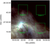 |
Fig. 1 UKIRT/WFCAM observed regions (square) overlayed on the Herschel three-color composite image (blue: 150, green: 250 and red: 500 μm). The regions are referred to as Region-1 to Region-4 starting from the southwest in a clockwise way, and the field of view is 13.75′ × 13.75′ for each region. In this paper, we focus on objects in Region-2, the most active star forming region. The northern half of Region-4 was regarded as an off-cloud reference field. |
2 Observations and analysis
We observed the R CrA region in the J-, H-, and K-bands using the United Kingdom Infrared Telescope (UKIRT) with the Wide Field CAMera (WFCAM; Casali et al. 2007) on 2010 August 8. The WFCAM has four Hawaii-II arrays (2048 × 2048 pixels; 13.75′ × 13.75′, total 756 arcmin2), which are referred to as channels 1–4 (hereafter Region-1 to Region-4) starting from the southwest in a clockwise way. Fig. 1 shows the observed WFCAM fields with a Herschel three-color composite image. The centers of the observation fields are summarized in Table 1.
The data were taken in the four-point jitter pattern and 10 × 2 point dithering with a 10 s exposure time per each filter. The average seeing size was ∼0.8′′. Dark subtraction, flat fielding, sky subtraction, and pixel scale conversion to 0.2′′ were processed by the CASU pipeline. The R CrA region, which is our main target in this paper was observed in Region-2. Region-4 where the globular cluster NGC 6723 is located has enough low cloud density to be regarded as “off-cloud”, so we used the northern half of Region-4 as a reference field. There are not any “off-cloud” YSOs reported in Galli et al. (2020) in the selected reference field, although a few of them are located within 1 square degree near the reference field. Thus, it is possible to estimate the contaminations of the target region. We performed PSF photometry using the Image Reduction and Analysis Facility (IRAF) DAOPHOT package. In order to detect all sources in the obtained image, both SExtractor (Bertin & Arnouts 1996) and the IRAF DAOFIND task were used since SExtractor has an advantage for the detection of overlapped and elliptical sources, while DAOFIND has a strength for the detection of sources located in the nebulous region. We then performed PSF photometry using the following steps. First, we performed PSF photometry on the images. Second, we subtracted the measured stars from the image. Third, we performed PSF photometry on the subtracted image. We repeated these steps a total of three times. After this, we detected sources with 3σ above the background in the stellar subtracted images using DAOFIND. We identified sources that were located within 1” at all JHK bands as a single object.
Photometric calibration was conducted by comparing the measured magnitudes with the 2MASS catalog (Skrutskie et al. 2006), which we converted to the WFCAM system by the equations from Hodgkin et al. (2009). In this calibration, we selected ∼30 2MASS stars that met the following two criteria: their magnitude errors are below 0.08 mag in each band and [J-H] < 2 mag. The magnitudes of the selected stars are J:12.0−16.0 mag, H: 12.0−16.0 mag, and K: 12.0−15.5 mag, and the difference between their coordinates is less than 1′′. Only [J-H] < 2 mag sources were selected in this photometric calibration since the color transformations depend on AV. The brighter objects (J, H ≤ 12.0 mag and K ≤ 11.0 mag) were replaced with the 2MASS magnitudes converted to the WFCAM system. We selected objects with a magnitude error ≤ J, H, and K of 0.3, 0.3, and 0.1 mag, respectively, for the following discussions. The total number of our identified sources is 2922. Table 2 shows the identified 2922 JHK sources in our survey, and 81 objects in the SIMBAD database are also shown in this table.
The 10 σ limiting magnitudes in the target and the reference fields are summarized in Table 3. They are about 2 mag deeper compared to the previous NIR surveys in the R CrA region (Haas et al. 2008). Fig. 2 presents the WFCAM JHK three-color composite image of the R CrA region. The Herbig Be star R CrA is the brightest in this region and it illuminates the surrounding nebulosity in the eastern region. Some bright Class I outflows and their nebula structures can also be seen in the eastern region. A dark lane is present between the region TY CrA and S CrA.
3 Results
3.1 Near-infrared sources and colors
3.1.1 Deriving the reddening law in [J-H]/[H-K] color-color diagram
Infrared extinction laws differ between the Galactic center region (e.g., Nishiyama et al. 2009) and star forming regions (e.g., Naoi et al. 2007) because of differences in dust grain size. Precise selection of YSO candidates with NIR excesses requires the application of the reddening law in each region with the individual photometric system. We note that steeper reddening lines are subject to the selection of many more NIR-excess sources composed of YSOs and background contaminations. In order to determine the reddening laws, we selected 2524 objects that were measured with S/N ≥ 10 in all of the JHK bands, and we derived color distributions on the [J-H]/[H-K] color-color diagram by binning their colors by 0.1 mag (Fig. 3).
Catalog of identified JHK sources.
Derived limiting magnitudes in target and reference fields.
We derived the reddening slope on the color-color diagrams by performing kernel density estimations using the “scipy.stat” (Virtanen et al. 2020) module “gaussian_kde” in the following steps. (1) We estimated the color distributions on the [J-H]/[H-K] diagram by performing kernel density estimations and drew contours in the logarithmic scale. (2) We estimated the most reddened position for each contour of the background star distribution. (3) We derived the reddening law using least-squares fitting of the most distant positions. We repeated these steps while changing the smoothness parameter of the contours (bw_method) from 0.5 to 0.9 in steps of 0.01 (examples for Fig. 4), and we determined a final slope of the reddening law from the least standard deviation (Fig. 5). The derived reddening law and fitting standard deviations for each bw_method are shown in Fig 5. The slope of the reddening law toward the R CrA region in the WFCAM system was determined to be E(J − H)/E(H − K) = 1.493 ± 0.009. Additionally, our JHK catalog was converted to the WFCAM system, which results in a difference in the reddening law from other photometric systems, such as the CIT system. On the assumption of AV = 0.412λ−1.75 (Tokunaga 2000), the E(J − H)/E(H − K) slope was determined to be 1.46 in the WFCAM system. In summary, taking into account these results, in this paper we adopted the reddening law of E(J − H)/E(H − K) = 1.5 for the R CrA region.
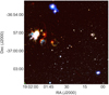 |
Fig. 2 UKIRT/WFCAM three-color composite image (blue: J, green: H and red: K-band) of the R CrA region. |
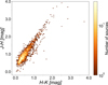 |
Fig. 3 Color distributions on the [J-H]/[H-K] color-color diagram of identified objects with S/N ≥ 10 in all the JHK bands. The distributions were derived by binning their colors by 0.1 mag. |
3.1.2 Selection of YSO candidates
As the observed colors were converted to the WFCAM system, the locus of main sequence stars and CTTS (Meyer et al. 1997; Oasa et al. 1999) were also converted from the CIT to the WFCAM system using relations from Hodgkin et al. (2009) and Carpenter (2001).
Fig. 6 shows the [J – H]/[H – K] color-color diagram of 2922 objects observed with S/N>10 at the K-band in the WFCAM system. On the [J – H]/[H – K] color-color diagram, objects with NIR excess were identified as YSO candidates. Identifications of Class I, II, and background objects on the [J – H]/[H – K] color-color diagram are based on Oasa et al. (1999). The YSOs with NIR excess should be distributed not only above the intrinsic CTTS locus but also below it since the locus was estimated using linear least-square fitting. We also identified objects located under the line within (J-H)=0.14 mag as Class II candidates. Table 4 shows the number of classified objects in the R CrA region. The detected objects in the R CrA region are more reddened than those in the reference field (Fig. 6 right), which distributed near the main sequence locus. Furthermore, the ratio of NIR-excess sources is higher in the R CrA region (9.5%) than in the reference field (6.7%).
Number of classified YSO and background candidates objects in the target field.
Number of classified Class II candidates.
The extinction and its error toward each source were determined based on the observed colors and errors. The extinction of the Class II candidates was derived from the distance between the observed colors and the intrinsic CTTS locus. The AV values were assumed as 0 mag for the Class II candidates located below the CTTS locus. For the background stars, we derived their extinctions the same way as Oasa et al. (2006). The uncertainty of these Av values was estimated from the [J-H] and [H-K] color errors. The derived extinction value reached up to Av ∼35 mag at the cluster center. In that region, there were fewer identified YSO candidates than in other regions. This means that there might be more reddened objects and faint YSO candidates that could not be detected from this observation, indicating that this cluster center is not only younger but also the densest cloud region of the Corona Australis cloud.
Fig. 8 shows the absolute J/[J – H] color-magnitude diagram of our identified Class II candidates in the R CrA region and the NIR-excess sources in the reference field. Class II candidates in the R CrA region are widely distributed due to the reddening, while NIR-excess sources in the reference field are concentrated around the isochrone. Since sources with NIR excess in the reference field are considered to be contaminated sources, their number in the R CrA region is estimated from the number of INR-excess sources identified in the reference region (see Section 4.1.1).
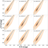 |
Fig. 4 Examples of the kernel density distributions of the [J-H]/[H-K] diagram with changing bw_method parameter. The bw_method values are from 0.5 to 0.9 and are shown in steps of 0.05 from the upper left to the bottom right. Gray distributions are the same as Fig. 3, and orange contours are derived kernel density distributions. Blue solid lines are estimated reddening vectors for each figure. |
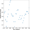 |
Fig. 5 Derived reddening slopes for each bw_method values. The bw_method values are from 0.5 to 0.9 with steps of 0.01. Error bars show standard deviations of each fitting. |
3.2 Deriving masses of Class II candidates
The masses of the Class II candidates were derived from their intrinsic J-band luminosities. This is because the J-band luminosities provide a more precise reflection of the stellar photosphere than the H- and K-band luminosities, which contain larger NIR excesses (Oasa et al. 2006). To determine the intrinsic J-band luminosities, the observed J-band magnitudes were corrected for individual extinctions and distance modulus. The luminosities of YSOs depend on their masses and ages. The masses of Class II objects were estimated from evolutionary models (e.g., Baraffe et al. 2015) by assuming an age of 1 Myr, which is typical for Class II objects. Then, we classified the candidates as LMSs (>0.08 M⊙), BDs (≤0.08 M⊙), and PMOs (≤0.013 M⊙) based on their estimated mass. The masses derived from the H-band luminosities were ∼13% larger than those from the J-band luminosities for all the Class II candidates (Fig. 7). This indicates that the H-band luminosities could contain not only the stellar photosphere but also some contributions of NIR excesses. Table 5 shows the number of Class II candidates by classification. Most of the detected candidates are identified as PMOs.
We compared our Class II candidates with unWISE (W1 and W2; Schlafly et al. 2019) data, allWISE (W3 and W4) data, Spitzer YSO candidates (IRAC1-4; Gutermuth et al. 2009; Peterson et al. 2011), and EL22 YSOs. Among our Class II candidates, 29, four, nine, and nine objects were cross-matched with these data that have high quality photometry, respectively. The total number of VLMO candidates in them is six (all of our BD candidates and one PMO candidate). We analyzed their spectral energy distributions (SEDs) using the Virtual Observatory Sed Analyzer (VOSA; Bayo et al. 2008) to estimate stellar physical parameters. Details about the SED analysis are summarized in the Appendix. For four of the six VLMO candidates, the SEDs exhibit clear evidence of NIR excesses, which is indicative of a circumstellar disk. As a result, we estimated the TSEDs of all six VLMO candidates to be 2500–3100 K, suggesting that they could be young BDs.
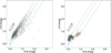 |
Fig. 6 Left: [J – H]/[H – K] color-color diagram of 2922 objects observed with S/N>10 at the K-band in the R CrA region. Circles and crosses show the objects identified as YSO candidates and background stars. Orange dashed lines show the intrinsic locus of CTTS, and blue solid and green solid lines show the intrinsic colors of main sequence stars and giants, respectively. An orange dash-dotted line shows the line that includes the 10σ color errors and reddening from the CTTS locus. Blue dotted lines represent the boundary of Class I and II, reddening vectors of main sequence stars and giant stars, from right to left. The black arrow shows the reddening vector of Av = 5. Right: [J – H]/[H – K] color-color diagram of the reference field. Lines and markers are the same as the color-color diagram of the R CrA region. The black arrow shows the reddening vector of Av = 5. |
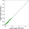 |
Fig. 7 Comparison of the masses of the Class II candidates derived from the J- and H-band luminosities. A dashed line represents where the J-masses are equal to the H-masses. The derived H-masses were ∼13% larger than the J-masses, suggesting that the H-band luminosities could contain some NIR excesses. |
4 Discussions
4.1 The initial mass functions
4.1.1 Subtraction of estimated contaminations
Our identified YSO candidates are considered to contain some background stars and galaxies, because they have NIR colors similar to those of CTTS. To evaluate the contributions of contaminated objects, we derived the contaminated mass function (MF) by estimating the number of NIR-excess sources identified in the off-cloud reference field (northern half of Region-4 in Fig. 1) using an artificially reddened [J – H]/[H – K] color-color diagram (Fig. 9). We note that there are no “off-cloud YSOs” of (Galli et al. 2020) in the selected reference field, but a few YSOs are located near the field. The Av is variable within the cloud, so we tried to classify the target region into four groups according to the cloud dust column density. We have estimated the contaminations for each group using the median Av value through the following steps. (1) We classified the R CrA region into four groups based on the Herschel dust column densities. (2) We derived a median Av value of background/Class III objects in each group. (3) We reddened the observed magnitudes of all sources in the reference field using a median Av value (2) for each group. (4) We identified objects with NIR excess that are brighter than the limiting magnitudes in the target region. (5) We estimated the masses of the identified (4) sources. (6) We constructed a contaminated MF considering the area ratio. The estimated number of the NIR-excess sources in the reference field for each column density is summarized in Table 6.
Number of classified YSO and background objects in the reference field.
We estimated the masses of objects classified as NIR-excess sources on the reddened color-color diagram in the reference field using the same method described in Section 3.2. All the derived masses of NIR-excess sources in the reference field are equivalent to PMOs. Sources whose luminosities correspond to the BDs are not identified in the reference color-color diagram. This indicates that there would not be contaminated background sources in the LMS and BD regimes. The contaminated MF was derived from the number of objects in each bin and then normalized to the size of the target region. There are objects only in the bins below the completeness limits where log(M*/M⊙) = −2.4 in the contaminated MF. We note that there is not any NIR-excess source whose parallax were measured by Gaia DR3. Thus, it is difficult to distinguish whether these NIR-excess sources are on-cloud YSOs or not. Additionally, there could be even more YSOs since our method can only identify YSOs showing the K-excess.
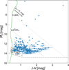 |
Fig. 8 Absolute J/[J – H] color-magnitude diagram of our identified Class II candidates in the R CrA region (blue circle) and the NIR-excess sources in the reference field (grey crosses). The green solid line and black arrow show the 1 Myr isochrone (Baraffe et al. 2015) and reddening vector of AV = 5 mag, respectively. The grey dotted and dash-dotted lines are the reddening lines of the LMS/BD and BD/PMO boundaries, respectively, and the gray dashed lines indicate the completeness limit. The brightest candidates, T CrA and S CrA, are not shown in this figure for better visibility. |
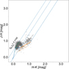 |
Fig. 9 Reddened [J – H]/[H – K] color-color diagram of the reference Group 1. All sources in the figure were reddened by Av = 2.4 mag along the reddening lines. The Av value represents the derived median value of background/Class III objects with their dust column density <1.2 × 10²¹/cm2 in the R CrA region. A black arrow shows the reddening vector of Av = 2.4 mag. Lines and markers in the figure are the same as in Fig. 6. |
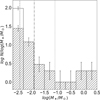 |
Fig. 10 Derived 1 Myr IMF in the R CrA region. Error bars represent the Poisson errors for each bin. Vertical dotted, dash-dotted, and dashed lines show the LMS/BD, BD/PMO boundaries and the completeness limit, respectively. The open histogram shows the IMF of all the sources, while the hatched histogram shows the IMF after subtracting the contaminated MF. |
4.1.2 Derived IMF
Our derived IMF of Class II candidates in the R CrA region are shown in Fig. 10. The completeness limit was determined from the dereddened limiting J0 magnitude in the target region. In the figure, we have subtracted the contaminated MF from the target MF for each bin.
The number of Class II candidates increases toward the completeness limit in the PMO regime. There is a small peak in the LMS regime, and the IMF appears to increase from the LMS/BD boundary to the BD/PMO boundary. The slope of the IMF can be regarded as flat when considered with the errors. However, the number of PMOs significantly increases from the BDs. We note that the determined background contaminated MF is likely an overestimate. Given this and the completeness, the derived IMF in the R CrA region would not decrease in the BD/PMO regime. Our derived IMF is similar to the IMF derived in ONC (Drass et al. 2016), although in ONC there is the first peak in the LMS regime (∼0.25 M⊙) and the second peak in the BD regime (∼0.025 M⊙), which is more massive than the second peak in the IMF of R CrA. The increasing features in the PMO regime in the R CrA IMF is similar to those (M* ≳ 0.01 M⊙) in ρ Oph (Marsh et al. 2010) and NGC1333 (Oasa et al. 2008). Those IMFs monotonously increase toward the PMO regime, unlike the R CrA IMF. The R CrA IMF shows a larger number of PMOs unlike open clusters (e.g., Jeffries 2012; Miret-Roig et al. 2022). This suggests that there might be environmental variations in the IMF, although there must be biases from observations and methods. We also estimated the masses of Class II candidates with age assumptions of 3 Myr and 5 Myr (Fig. 11), but there were no significant differences between them. It is important to confirm VLMO candidates by spectroscopic observations in order to obtain more detailed and precise comparisons of IMFs, and we propose this as a next step.
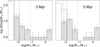 |
Fig. 11 Derived 3 Myr (left) and 5 Myr (right) IMFs in the R CrA region. Lines are the same as in the Fig. 10. We note that the last two bins in the 5 Myr IMF are less reliable due to a more massive mass-completeness limit. |
4.2 Comparing YSO candidates with cloud properties
4.2.1 Spatial distributions of YSO candidates
We compared the spatial distributions of our identified YSO candidates with the Herschel dust column density (Bresnahan et al. 2018) in Fig. 12. Class I candidates are concentrated in the cloud core (≥10 × 1021/cm2), which is called the “coronet cluster.” There is also the Herbig Ae star R CrA and some PMO candidates. The BD candidates are not identified in the cloud core region, while the PMO candidates have been identified there. The PMO candidates are more distributed in the low to high dust density regions than other YSO candidates. Most of the LMS candidates and BD candidates are located in the southern part of the cloud, where the dust density is intermediate (∼3−10 × 1021/cm2). In addition, most of the LMS candidates are located in higher dust density regions (≳ 5 × 10²¹/cm2) compared to BD candidates (∼4 × 10²¹/cm2). Also, lower mass BD and LMS candidates are located in the higher dust density regions compared to candidates with a higher mass. This suggests that the YSO distribution cloud be dependent on the local dust density in the R CrA region.
4.2.2 Comparing derived mass of YSO candidates with the Herschel dust column density
We compared the estimated mass of our YSO candidates with the Herschel dust column density of the molecular cloud to quantitatively examine the relations between the YSO mass and the local dust density. Fig. 13 shows a comparison between the estimated mass of our YSO candidates and their local dust density for the same source. The completeness limit is derived from the 10σ limiting J mag with an average AJ in the observed region.
The mean values of the local dust column density are estimated as NH2 = 16, 9.2, and 3.9 × 10²¹/cm2 for LMS, BD, and PMO candidates. Our survey is deep enough to identify ∼10 MJ PMO ages at 1 Myr, which suffer from AV ∼20 mag (NH2 ∼2.0 × 10²²/cm2). We note that it is possible that there exists more PMOs in the dense cloud core. All the identified LMS candidates and BD candidates are located in the higher (≥2.5 × 10²¹/cm2) dust density regions, while PMO candidates are independent of their local dust densities. This indicates that LMSs and BDs might be formed in regions with higher dust density. For PMO candidates, it has been suggested that they could be formed even in the low dust density, although the probability of background contaminations, such as distant galaxies and active galactic nuclei, become higher for the lower dust density regions. This indicates the formations of very LMSs (M* ≲ 0.5 M⊙) and VLMOs could be dependent on the local cloud properties.
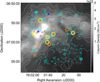 |
Fig. 12 Spatial distribution of the identified YSO candidates in the R CrA region. Yellow, orange, cyan and red circles represent identified LMS, BD, PMO, and Class I candidates, respectively. Objects with their luminosity below the completeness limit are shown as small cyan circles. Blue star symbols show positions of young early-type stars named R CrA and TY CrA that are not among our YSO candidates. Solid contours show the Herschel dust column density distribution where 1, 2, 3, 4, 5, 6, 7, 8, 9, 10, 15, 20, 25, 30, 35, 40, 45, 50 × 1021/cm2. |
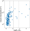 |
Fig. 13 Mass of YSO candidates versus dust column density determined from Herschel. Vertical dotted, dash-dotted and dashed lines show the LMS/BD, BD/PMO boundaries and completeness limit, respectively. Gray dots represent objects with a mass below the completeness limit, while blue circles represent those above it. |
5 Summary
We have conducted deep JHK photometric survey using UKIRT/WFCAM to identify VLMO candidates in the nearby star forming region R CrA. We summarize our main results as follows:
The 10 σ limiting magnitudes were 20.7, 19.6, and 19.2 mag in the J-, H-, and K-band, respectively. They are more than 3 mag deeper than the previous JHK survey in the R CrA region (Haas et al. 2008). Our survey identified 2922 JHK sources in all the JHK bands.
We identified 222 Class I and II candidates (Class I: 15; Class II: 207) with NIR excess from the [J-H]/[H-K] colorcolor diagram.
Masses of Class II candidates were estimated from the dereddend J-band luminosities with an age assumption of 1 Myr using the evolutionary models. Six LMS candidates, five BD candidates, and 198 PMO candidates were identified.
We derived the IMF down to the PMO regime (M* ≲ 0.01 M⊙) in the R CrA region, which is subtracted the expected contaminations. The number of PMOs is larger than that of BDs. The derived IMF does not appear to decrease in the BD and PMO regime, even when taking into account of the background star and galactic contamination.
We compared the spatial distribution of our identified Class I and II candidates with dust column densities derived from the Herschel observation. The PMO candidates are located in the low to high dust density regions (∼1−20 × 1021/cm2), while BD candidates are located in the intermediate dust density regions (∼3−10 × 1021/cm2).
We compared the derived mass of Class II candidates to the dust density of their positions. All the LMS candidates and BD candidates are located in the relatively higher (≥2.5 × 10²¹/cm2) dust density regions, while PMO candidates are independent of their local dust densities.
Data availability
Full Table 2 is available at the CDS via anonymous ftp to cdsarc.cds.unistra.fr (130.79.128.5) or via https://cdsarc.cds.unistra.fr/viz-bin/cat/J/A+A/698/A96
Acknowledgements
We thank Dr. T. Kudo and Dr. Y. Saito for helping UKIRT/WFCAM observations. We are grateful to Dr. Y. Itoh for helpful discussions. We are also grateful to the anonymous referee for helpful comments on the original manuscript that improved the discussion of this work.
This work was supported by the Japan Society for the Promotion of Science (JSPS) KAKENHI Grant Number 25870124, 17K00960, 17K05390 and 22 K 03677. UKIRT is owned by the University of Hawaii (UH) and operated by the UH Institute for Astronomy. When the data reported here were obtained, UKIRT was operated by the Joint Astronomy Centre on behalf of the Science and Technology Facilities Council of the U.K. This research has made use of the SIMBAD database, operated at CDS, Strasbourg, France. This work made use of Astropy1: a community-developed core Python package and an ecosystem of tools and resources for astronomy (Astropy Collaboration 2013, 2018, 2022). This research made use of APLpy (Robitaille & Bressert 2012), an open-source plotting package for Python. This publication makes use of VOSA, developed under the Spanish Virtual Observatory (https://svo.cab.inta-csic.es) project funded by MCIN/AEI/10.13039/501100011033/through grant PID2020-112949GB-I00. VOSA has been partially updated by using funding from the European Union’s Horizon 2020 Research and Innovation Programme, under Grant Agreement no. 776403 (EXOPLANETS-A).
Appendix A Known members of Class II candidates
We compared our Class II candidates with unWISE (W1 and W2; Schlafly et al. 2019) data, allWISE (W3 and W4) data, Spitzer YSO candidates (IRAC1-4; Gutermuth et al. 2009; Peterson et al. 2011), and EL22 YSOs. Among our Class II candidates, 29, four, nine, and nine objects were cross-matched with these data that have high quality photometry, respectively.
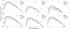 |
Fig. A.1 Derived SEDs of our BD and PMO candidates. Green, yellow, orange, and red circles represent optical (SDSS and/or Gaia), our JHK photometry, unWISE(Schlafly et al. 2019), and Spitzer data. Open triangles in the figure show that the AllWISE upper limit. Error bars are smaller than the symbol size. Blue and gray solid line shows the best fitted flux and spectrum of the BT-Settl model (Caffau et al. 2011). The source ID and the derived parameters are shown in the upper right of figures. The TSED was determined from the fluxes in the wavelength shorter than the vertical dashed line. |
The observed SED in the optical (SDSS and/or Gaia, if available) and the NIR for each object is compared to the synthetic photometry for BT-settle (CIFIST2011) models (Caffau et al. 2011) suitable for LMS using a chi-square test. In this analysis, we require that the objects have high quality photometries all in JHK, W1-2 and IRAC1-4. The total number of VLMOs fulfilling this criterion is six (all of our BD candidates and one PMO candidate). To estimate stellar physical parameters, we have used the Virtual Observatory Sed Analyzer (VOSA Bayo et al. 2008) as follows: (1) give an Av in the range of our derived Av ± 1.5 mag and the log g was assumed to 3.5−4, since the surface gravity of YSOs show intermediate values between those of main sequence and giants (e.g. Takagi et al. 2011) (2) fit the SED models to the objects without defining the NIR excess (3) if the fitting results do not show the significant NIR excess, we adopted photometry from optical to 5 μm (4) if the NIR excess was detected, we adopted photometry from optical to 5 μm to 3.6−5 μm to search best fit parameters The derived best fit SEDs are shown in Fig. A.1. For four of six very VLMO candidates, the SED exhibit clear evidence of NIR excesses, indicative of the circumstellar disks. Derived parameters of our VLMO candidates from VOSA SED fitting and previous NIR spectroscopy (EL22) are summarized in Table A.1.
Derived VLMO candidate parameters from VOSA SED fitting.
The derived TSED of all five BD candidates are similar to the spectral types identified by NIR spectroscopy (EL22). Both our SED fitting and EL22 spectral analysis indicate that they are cool (TSED = 2500−3100 K) objects. These low temperatures suggest that these BD candidates cloud be young BDs. In our PMO candidates, only #2058 is found in the YSO list of EL22. Their identified spectral type of #2058 is identified as M6. From our SED fitting, the TSED is determined to be 3100 K, slightly higher than EL22, and the NIR excess is clearly detected from 3.4 μm. Combined with the TSED = 3100 K or M6, this object appears to be a young BD older than 3 Myr. In addition, for our LMS candidates, spectral types of our LMS candidates, #2066, #2315 and #2595 are identified as M3, M2 and M8, respectively (EL22). For #2596, our photometric mass is derived to be 0.093 M⊙. T CrA (#2777) and S CrA (#741), well known a F-type LMS (Manoj et al. 2006) and a G-type LMS (Carmona et al. 2007), respectively, and IRS 2 (#2314), also known as a Class I object (e.g. Forbrich & Preibisch 2007), are also selected as LMS candidates in our method. We note that the magnitudes of the brighter LMS candidates are replaced to the 2MASS catalogue.
In summary, seven of our eight LMS/BD candidates and one PMO candidate have been spectroscopically confirmed as YSOs located in the R CrA region. In addition, TSED of six VLMO candidates were estimated as low temperatures similar to the spectral types of EL22. For four of the six VLMO candidates, the SEDs exhibit clear evidence of NIR excesses, which is indicative of a circumstellar disk.
References
- Astropy Collaboration (Robitaille, T. P., et al.,) 2013, A&A, 558, A33 [NASA ADS] [CrossRef] [EDP Sciences] [Google Scholar]
- Astropy Collaboration (Price-Whelan, A. M., et al.,) 2018, AJ, 156, 123 [Google Scholar]
- Astropy Collaboration (Price-Whelan, A. M., et al.,) 2022, ApJ, 935, 167 [NASA ADS] [CrossRef] [Google Scholar]
- Baraffe, I., Homeier, D., Allard, F., & Chabrier, G., 2015, A&A, 577, A42 [NASA ADS] [CrossRef] [EDP Sciences] [Google Scholar]
- Bate, M. R., Bonnell, I. A., & Bromm, V., 2002, MNRAS, 332, L65 [NASA ADS] [CrossRef] [Google Scholar]
- Bayo, A., Joergens, V., Liu, Y., et al. 2017, ApJ, 841, L11 [Google Scholar]
- Bayo, A., Rodrigo, C., Barrado Y Navascués, D., et al. 2008, A&A, 492, 277 [NASA ADS] [CrossRef] [EDP Sciences] [Google Scholar]
- Bertin, E., & Arnouts, S., 1996, A&AS, 117, 393 [NASA ADS] [CrossRef] [EDP Sciences] [Google Scholar]
- Bresnahan, D., Ward-Thompson, D., Kirk, J. M., et al. 2018, A&A, 615, A125 [NASA ADS] [CrossRef] [EDP Sciences] [Google Scholar]
- Caffau, E., Ludwig, H. G., Steffen, M., Freytag, B., & Bonifacio, P., 2011, Sol. Phys., 268, 255 [Google Scholar]
- Carmona, A., van den Ancker, M. E., & Henning, T., 2007, A&A, 464, 687 [NASA ADS] [CrossRef] [EDP Sciences] [Google Scholar]
- Carpenter, J. M., 2001, AJ, 121, 2851 [Google Scholar]
- Casali, M., Adamson, A., Alves de Oliveira, C., et al. 2007, A&A, 467, 777 [NASA ADS] [CrossRef] [EDP Sciences] [Google Scholar]
- Choi, M., Tatematsu, K., Hamaguchi, K., & Lee, J.-E., 2009, ApJ, 690, 1901 [Google Scholar]
- Drass, H., Haas, M., Chini, R., et al. 2016, MNRAS, 461, 1734 [NASA ADS] [CrossRef] [Google Scholar]
- Esplin, T. L., & Luhman, K. L., 2022, AJ, 163, 64 [NASA ADS] [CrossRef] [Google Scholar]
- Forbrich, J., & Preibisch, T., 2007, A&A, 475, 959 [NASA ADS] [CrossRef] [EDP Sciences] [Google Scholar]
- Galli, P. A. B., Bouy, H., Olivares, J., et al. 2020, A&A, 634, A98 [NASA ADS] [CrossRef] [EDP Sciences] [Google Scholar]
- Gray, R. O., Corbally, C. J., Garrison, R. F., et al. 2006, AJ, 132, 161 [Google Scholar]
- Gutermuth, R. A., Megeath, S. T., Myers, P. C., et al. 2009, ApJS, 184, 18 [Google Scholar]
- Haas, M., Heymann, F., Domke, I., et al. 2008, A&A, 488, 987 [NASA ADS] [CrossRef] [EDP Sciences] [Google Scholar]
- Hodgkin, S. T., Irwin, M. J., Hewett, P. C., & Warren, S. J., 2009, MNRAS, 394, 675 [CrossRef] [Google Scholar]
- Jeffries, R. D., 2012, in EAS Publications Series, 57, eds. C. Reylé, C. Charbonnel, & M. Schultheis, 45 [Google Scholar]
- Luhman, K. L., 2012, ARA&A, 50, 65 [CrossRef] [Google Scholar]
- Luhman, K. L., Alves de Oliveira, C., Baraffe, I., et al. 2024, AJ, 167, 19 [Google Scholar]
- Manoj, P., Bhatt, H. C., Maheswar, G., & Muneer, S., 2006, ApJ, 653, 657 [Google Scholar]
- Marsh, K. A., Plavchan, P., Kirkpatrick, J. D., et al. 2010, ApJ, 719, 550 [NASA ADS] [CrossRef] [Google Scholar]
- Martín, E. L., Žerjal, M., Bouy, H., et al. 2025, A&A, 697, A7 [NASA ADS] [CrossRef] [EDP Sciences] [Google Scholar]
- Meyer, M. R., Calvet, N., & Hillenbrand, L. A., 1997, AJ, 114, 288 [Google Scholar]
- Miret-Roig, N., Bouy, H., Raymond, S. N., et al. 2022, Nat. Astron., 6, 89 [NASA ADS] [CrossRef] [Google Scholar]
- Naoi, T., Tamura, M., Nagata, T., et al. 2007, ApJ, 658, 1114 [Google Scholar]
- Neuhäuser, R., & Forbrich, J., 2008, in Handbook of Star Forming Regions, Volume II, 5, ed. B. Reipurth, 735 [Google Scholar]
- Nishiyama, S., Tamura, M., Hatano, H., et al. 2009, ApJ, 696, 1407 [NASA ADS] [CrossRef] [Google Scholar]
- Oasa, Y., Tamura, M., & Sugitani, K., 1999, ApJ, 526, 336 [NASA ADS] [CrossRef] [Google Scholar]
- Oasa, Y., Tamura, M., Nakajima, Y., et al. 2006, AJ, 131, 1608 [Google Scholar]
- Oasa, Y., Tamura, M., Sunada, K., & Sugitani, K., 2008, AJ, 136, 1372 [Google Scholar]
- Offner, S. S. R., Clark, P. C., Hennebelle, P., et al. 2014, in Protostars and Planets VI, eds. H. Beuther, R. S. Klessen, C. P. Dullemond, & T. Henning, 53 [Google Scholar]
- Olofsson, G., Huldtgren, M., Kaas, A. A., et al. 1999, A&A, 350, 883 [NASA ADS] [Google Scholar]
- Peterson, D. E., Caratti o Garatti, A., Bourke, T. L., et al. 2011, ApJS, 194, 43 [NASA ADS] [CrossRef] [Google Scholar]
- Robitaille, T., & Bressert, E., 2012, APLpy: Astronomical Plotting Library in Python, Astrophysics Source Code Library [record ascl:1208.017] [Google Scholar]
- Schlafly, E. F., Meisner, A. M., & Green, G. M., 2019, ApJS, 240, 30 [Google Scholar]
- Skrutskie, M. F., Cutri, R. M., Stiening, R., et al. 2006, AJ, 131, 1163 [NASA ADS] [CrossRef] [Google Scholar]
- Takagi, Y., Itoh, Y., Oasa, Y., & Sugitani, K., 2011, PASJ, 63, 677 [Google Scholar]
- Taylor, K. N. R., & Storey, J. W. V., 1984, MNRAS, 209, 5 [Google Scholar]
- Tokunaga, A. T., 2000, in Allen’s Astrophysical Quantities, ed. A. N. Cox, 143 [Google Scholar]
- Vaytet, N., & Haugbølle, T., 2017, A&A, 598, A116 [NASA ADS] [CrossRef] [EDP Sciences] [Google Scholar]
- Virtanen, P., Gommers, R., Oliphant, T. E., et al. 2020, Nat. Methods, 17, 261 [Google Scholar]
- Wilking, B. A., McCaughrean, M. J., Burton, M. G., et al. 1997, AJ, 114, 2029 [Google Scholar]
All Tables
All Figures
|
Fig. 1 UKIRT/WFCAM observed regions (square) overlayed on the Herschel three-color composite image (blue: 150, green: 250 and red: 500 μm). The regions are referred to as Region-1 to Region-4 starting from the southwest in a clockwise way, and the field of view is 13.75′ × 13.75′ for each region. In this paper, we focus on objects in Region-2, the most active star forming region. The northern half of Region-4 was regarded as an off-cloud reference field. |
| In the text | |
|
Fig. 2 UKIRT/WFCAM three-color composite image (blue: J, green: H and red: K-band) of the R CrA region. |
| In the text | |
|
Fig. 3 Color distributions on the [J-H]/[H-K] color-color diagram of identified objects with S/N ≥ 10 in all the JHK bands. The distributions were derived by binning their colors by 0.1 mag. |
| In the text | |
|
Fig. 4 Examples of the kernel density distributions of the [J-H]/[H-K] diagram with changing bw_method parameter. The bw_method values are from 0.5 to 0.9 and are shown in steps of 0.05 from the upper left to the bottom right. Gray distributions are the same as Fig. 3, and orange contours are derived kernel density distributions. Blue solid lines are estimated reddening vectors for each figure. |
| In the text | |
|
Fig. 5 Derived reddening slopes for each bw_method values. The bw_method values are from 0.5 to 0.9 with steps of 0.01. Error bars show standard deviations of each fitting. |
| In the text | |
|
Fig. 6 Left: [J – H]/[H – K] color-color diagram of 2922 objects observed with S/N>10 at the K-band in the R CrA region. Circles and crosses show the objects identified as YSO candidates and background stars. Orange dashed lines show the intrinsic locus of CTTS, and blue solid and green solid lines show the intrinsic colors of main sequence stars and giants, respectively. An orange dash-dotted line shows the line that includes the 10σ color errors and reddening from the CTTS locus. Blue dotted lines represent the boundary of Class I and II, reddening vectors of main sequence stars and giant stars, from right to left. The black arrow shows the reddening vector of Av = 5. Right: [J – H]/[H – K] color-color diagram of the reference field. Lines and markers are the same as the color-color diagram of the R CrA region. The black arrow shows the reddening vector of Av = 5. |
| In the text | |
|
Fig. 7 Comparison of the masses of the Class II candidates derived from the J- and H-band luminosities. A dashed line represents where the J-masses are equal to the H-masses. The derived H-masses were ∼13% larger than the J-masses, suggesting that the H-band luminosities could contain some NIR excesses. |
| In the text | |
|
Fig. 8 Absolute J/[J – H] color-magnitude diagram of our identified Class II candidates in the R CrA region (blue circle) and the NIR-excess sources in the reference field (grey crosses). The green solid line and black arrow show the 1 Myr isochrone (Baraffe et al. 2015) and reddening vector of AV = 5 mag, respectively. The grey dotted and dash-dotted lines are the reddening lines of the LMS/BD and BD/PMO boundaries, respectively, and the gray dashed lines indicate the completeness limit. The brightest candidates, T CrA and S CrA, are not shown in this figure for better visibility. |
| In the text | |
|
Fig. 9 Reddened [J – H]/[H – K] color-color diagram of the reference Group 1. All sources in the figure were reddened by Av = 2.4 mag along the reddening lines. The Av value represents the derived median value of background/Class III objects with their dust column density <1.2 × 10²¹/cm2 in the R CrA region. A black arrow shows the reddening vector of Av = 2.4 mag. Lines and markers in the figure are the same as in Fig. 6. |
| In the text | |
|
Fig. 10 Derived 1 Myr IMF in the R CrA region. Error bars represent the Poisson errors for each bin. Vertical dotted, dash-dotted, and dashed lines show the LMS/BD, BD/PMO boundaries and the completeness limit, respectively. The open histogram shows the IMF of all the sources, while the hatched histogram shows the IMF after subtracting the contaminated MF. |
| In the text | |
|
Fig. 11 Derived 3 Myr (left) and 5 Myr (right) IMFs in the R CrA region. Lines are the same as in the Fig. 10. We note that the last two bins in the 5 Myr IMF are less reliable due to a more massive mass-completeness limit. |
| In the text | |
|
Fig. 12 Spatial distribution of the identified YSO candidates in the R CrA region. Yellow, orange, cyan and red circles represent identified LMS, BD, PMO, and Class I candidates, respectively. Objects with their luminosity below the completeness limit are shown as small cyan circles. Blue star symbols show positions of young early-type stars named R CrA and TY CrA that are not among our YSO candidates. Solid contours show the Herschel dust column density distribution where 1, 2, 3, 4, 5, 6, 7, 8, 9, 10, 15, 20, 25, 30, 35, 40, 45, 50 × 1021/cm2. |
| In the text | |
|
Fig. 13 Mass of YSO candidates versus dust column density determined from Herschel. Vertical dotted, dash-dotted and dashed lines show the LMS/BD, BD/PMO boundaries and completeness limit, respectively. Gray dots represent objects with a mass below the completeness limit, while blue circles represent those above it. |
| In the text | |
|
Fig. A.1 Derived SEDs of our BD and PMO candidates. Green, yellow, orange, and red circles represent optical (SDSS and/or Gaia), our JHK photometry, unWISE(Schlafly et al. 2019), and Spitzer data. Open triangles in the figure show that the AllWISE upper limit. Error bars are smaller than the symbol size. Blue and gray solid line shows the best fitted flux and spectrum of the BT-Settl model (Caffau et al. 2011). The source ID and the derived parameters are shown in the upper right of figures. The TSED was determined from the fluxes in the wavelength shorter than the vertical dashed line. |
| In the text | |
Current usage metrics show cumulative count of Article Views (full-text article views including HTML views, PDF and ePub downloads, according to the available data) and Abstracts Views on Vision4Press platform.
Data correspond to usage on the plateform after 2015. The current usage metrics is available 48-96 hours after online publication and is updated daily on week days.
Initial download of the metrics may take a while.