| Issue |
A&A
Volume 698, May 2025
|
|
|---|---|---|
| Article Number | A123 | |
| Number of page(s) | 13 | |
| Section | Extragalactic astronomy | |
| DOI | https://doi.org/10.1051/0004-6361/202449878 | |
| Published online | 03 June 2025 | |
Multifrequency simultaneous VLBA view of the radio source 3C 111
1
Max-Planck-Institut für Radioastronomie, Auf dem Hügel 69, D-53121 Bonn, Germany
2
Dipartimento di Fisica e Astronomia, Università degli Studi di Bologna, Via Gobetti 93/2, I-40129 Bologna, Italy
3
Instituto de Astrofísica de Andalucía-CSIC, Glorieta de la Astronomía s/n, E-18008 Granada, Spain
4
INAF – Istituto di Radioastronomia, Via Gobetti 101, I-40129 Bologna, Italy
⋆ Corresponding author.
Received:
6
March
2024
Accepted:
24
March
2025
Context. Relativistic jets originating at the center of active galactic nuclei are embedded in extreme environments with strong magnetic fields and high particle densities, which makes them a fundamental tool for studying the physics of magnetized plasmas.
Aims. We aim to investigate the magnetic field structure and the parsec and sub-parsec properties of the relativistic jet in the radio galaxy 3C 111. Rotation measure (RM) studies of nearby radio-galaxies, such as this one, provide a valuable tool with which to investigate the transversal magnetic field properties.
Methods. We used multifrequency simultaneous Very Long Baseline Array (VLBA) data from 5 GHz up to 87.6 GHz. We performed an analysis of both total intensity and polarization maps to study the jet magnetic field and infer the spectral properties of the synchrotron emission. We modeled the brightness distribution of the source with multiple 2D Gaussian components to characterize individual emission features.
Results. After determining the core shift (rc ∝ ν−1.27 ± 0.17), we computed the spectral index maps for all the adjacent frequency pairs and found different distributions for the core region (αmax ≈ 1.5 and αmin ≈ 0.2) and the jet (α ≈ −1.5 on average) with an unusual optically thick or flat feature in it at ≈1 − 2 pc from the core. Using modelfit, we found a total of 56 components at different frequencies. By putting constraints on the size and position, we identified 22 components at different frequencies for which we computed the equipartition magnetic field. We computed the rotation measure at two different triplets of frequencies. At 15.2 − 21.9 − 43.8 GHz, we discovered high values of RM in the same region where the optically thick or flat feature was found. This can be associated with a high electron density value at ≈1 − 2 pc from the core that we interpret as originating in a cloud of the clumpy torus. At 5 − 8.4 − 15.2 GHz, we found a distribution of the electric vector position angles and significant RM transverse gradient that provide strong evidence of a helical configuration of the magnetic field, as found in simulations.
Key words: galaxies: active / galaxies: individual: 3C111 / galaxies: jets / galaxies: magnetic fields / galaxies: nuclei
© The Authors 2025
 Open Access article, published by EDP Sciences, under the terms of the Creative Commons Attribution License (https://creativecommons.org/licenses/by/4.0), which permits unrestricted use, distribution, and reproduction in any medium, provided the original work is properly cited.
This article is published in open access under the Subscribe to Open model.
Open Access funding provided by Max Planck Society.
1. Introduction
Active galactic nuclei (AGNi) are some of the most interesting astronomical objects among the ones observable using the Very Long Baseline Interferometer (VLBI) technique. They are excellent laboratories for a variety of physical processes. The standard model of AGNi suggests the presence of a supermassive black hole (SMBH) at the center of the galaxy, which accretes matter and can be surrounded by an obscuring torus (Urry & Padovani 1995). The complex dynamics around the SMBH and the presence of intense magnetic fields may lead to the production of two relativistic plasma streams of charged particles, emitting nonthermal radiation, called jets, propagating in opposite directions to each other. Radio galaxies (RGs) are defined as AGNi with jets at a large angle to the line of sight and, among RGs, Fanaroff & Riley (1974) suggested a division based on their morphology and radio luminosity. FR I RGs have lower power (i.e., P1.4 GHz < 1024.5 W/Hz) and their emission on kiloparsec scales is dominated by their jet; FR II RGs, on the other hand, have high power (i.e., P1.4 GHz > 1024.5 W/Hz) and are dominated on large scales by hotspots; that is, regions in which a jet terminates due to an interaction with the intergalactic medium (IGM). The emission from RGs spans the whole electromagnetic spectrum, from the radio domain to γ-rays (e.g., Casadio et al. 2015; Grandi et al. 2012). Nonthermal radiation is mainly produced by charged particles, that is, leptons interacting with each other (e.g., via scattering processes) and with the magnetic field in the jet (e.g., synchrotron emission). Therefore, properly characterizing the particle population and the magnetic field intensity and distribution is crucial to understanding the physics of AGNi. Thanks to the VLBI technique, it is possible to resolve radio jets down to event horizon scales (Event Horizon Telescope Collaboration 2019), and therefore it is one of the best tools for studying the jet structure and evolution.
Synchrotron emission from AGN jets is polarized. Therefore, with a simultaneous multifrequency dataset, it is possible to infer the rotation measure (RM) structure (see e.g., Hovatta et al. 2012, for a complete review of the topic), and thus the Faraday-corrected magnetic field distribution in a certain region of the jet.
Relativistic magnetohydrodynamic (RMHD) simulations of AGN jets can successfully reproduce different magnetic field configurations based on different types of environmental and intrinsic AGN properties (e.g., Perucho 2019). Hence, high-resolution VLBI observations of polarized AGN jets, along with RMHD simulations, are fundamental to shed light on the accretion and ejection mechanisms from SMBHs. In this paper, we focus on an interesting case study: the broad-line RG (BLRG) 3C 111.
In the radio domain, 3C 111 is classified as an FR II RG, presenting two radio lobes and a single-sided jet. The jet lies at an angle of ≈17° with respect to the line of sight (Jorstad et al. 2017). On parsec scales, the counter-jet is not detected, likely due to Doppler deboosting (Chatterjee et al. 2011). The radio core is highly compact and bright, and on parsec scales the jet has a blazar-like behavior, showing apparent superluminal motion (e.g., Beuchert et al. 2018), at odds with the kiloparsec-scale morphology (Linfield & Perley 1984). In addition to these features, given its proximity, VLBI observations of 3C 111 (z = 0.049) (Véron-Cetty & Véron 2006) down to millimeter wavelengths enable us to probe the jet base with a high spatial resolution and reduced opacity effects, and thus to investigate the magnetic field geometry and nuclear environment within the jet collimation region (Kovalev et al. 2020).
The main aim of this work is to study the physics and magnetic field structure in the parsec-scale jet of 3C 111. This source has been widely studied throughout the years, both from an observational point of view (e.g., Kadler et al. 2008; Beuchert et al. 2018; Schulz et al. 2020) and with the help of simulations (e.g., Perucho et al. 2008; Fichet de Clairfontaine et al. 2022). Our work fits into this context thanks to our simultaneous observation that span six different frequencies, providing the chance to study the jet structure from parsec to sub-parsec scales. This paper is organized as follows. In Sect. 2, we describe the calibration of the dataset used in this work. In Sect. 3, we produce maps for all the available frequencies, both in total and polarization intensity. After correcting for the core-shift, we produce the spectral index distribution for all the frequency pairs. In Sect. 4, we explore the relation between the physical parameters associated with the different modelfit components (e.g., the magnetic field) and we retrieve RM maps for two different triplets of frequency.
In this paper, we assume a ΛCDM cosmology with H0 = 69.6 km s−1 Mpc−1, ΩM = 0.286, and ΩΛ = 0.714 (Bennett et al. 2014). At the redshift of 3C 111, the luminosity distance is DL = 214 Mpc, and the angular size of 1 mas corresponds to a linear size of ≈0.95 pc.
2. Dataset and calibration
In this work, we analyze a set of multi-wavelength radio observations obtained with the Very Long Baseline Array (VLBA) on May 8, 2014. The dataset spans seven different frequencies: 1.4 GHz (L band), 5 GHz (C band), 8.4 GHz (X band), 15.2 GHz (U band), 21.9 GHz (K band), 43.8 GHz (Q band), and 87.6 GHz (W band). Each observing frequency is divided into eight IFs (Intermediate Frequencies) with a bandwidth of 32 MHz and a channel separation of 500 kHz, producing a total bandwidth per polarization of 256 MHz. The total on-source time is 15.6 m for the C band, 9.1 m for the X band, 20.5 m for the U band, 147.9 m for the K band, 54.6 m for the Q band, and 55.1 for the W band. The recorded data rate at each band is 2 Gbit/s. Due to a reduced number of scans, we did not include the 1.4 GHz data in the analysis. During the observations, North Liberty was not observing due to technical problems, leaving nine telescopes observing. To analyze and calibrate the data, we used ParselTongue (Kettenis et al. 2006), a Python interface of AIPS, the Astronomical Image Processing System (Greisen et al. 2003). For the calibration of the dataset, we made use of a routine developed by J. L. Gómez and A. Fuentes that follows the standard procedures for polarization observations (e.g., Jorstad et al. 2005). At this stage, it is possible to perform the imaging process with Difmap (Shepherd 1997). We used the CLEAN deconvolution algorithm (Högbom 1974) along with self-calibration procedures in order to produce the total intensity images. After producing the spectrum of 3C 111 integrated over the whole source, we noticed that the 21.9 GHz flux was lower than expected. We inspected the integrated spectrum for other known flux density calibrators (e.g., 3C 84) and found the same scaling issue. Namely, the K-band flux density was ≈20% lower than expected in all the sources, suggesting a possible issue in the observation. We noticed that for some scans, some baselines (e.g., the ones involving Brewster or Hancock) were dragging the average amplitude down. Therefore, we flagged those baselines and proceeded with the amplitude self-calibration without said antennas. Then, we used the obtained model to scale all the antennas. We then performed the polarimetry calibration by uploading the total intensity images in ParselTongue. We used the AIPS task LPCAL to determine the instrumental polarization generally referred to as “D-terms” polarization leakages (see, e.g. Casadio et al. 2019, for an extended description). We found leakages in the range of a few percent, with values progressively higher with frequency, but all below 10%. To correct for the absolute orientation of the electric vector position angles (EVPAs), we considered the appropriate frequency data from the FGAMMA program (Angelakis et al. 2019, 5 GHz and 8.4 GHz), the MOJAVE database (15.2 GHz), and the VLBA-BU-BLAZAR Program1 for 43 GHz. We interpolated the data for the EVPA at 21.9 GHz and extrapolated those at 87.6 GHz, the latter therefore being quite uncertain and needing to be handled with care.
To perform a discrete analysis of the jet emission, we modeled its brightness distribution at each frequency as a set of 2D circular Gaussian components through the modelfit function in Difmap, following the approach by Lico et al. (2012). This was done to better characterize the jet structure and to try to recognize the same features at different frequencies (see Sect. 4.2). To prevent the fitting procedure from modeling components that are not physically realistic in order to reach a better convergence, we fixed the size of each component to 0.1 of the beam minor axis whenever a component was shrunk to a size smaller than 10% of the beam minor axis. When the latter happened, we treated the sizes of such components as upper limits. We estimated the uncertainties of the modelfit flux, ΔF(ν), with Eq. (1):

where the first term (10% F(ν)) is a conservative choice that represents the calibration error and 3σrms is 3 times the off-source root mean square (rms) noise of the map, representing the statistical error as was done in previous studies (e.g., Lico et al. 2012). The uncertainties on the position and size of the components were estimated based on the approach followed by Orienti et al. (2011). Namely, for the position, we estimated Δr as Δr = θ/SNR, where θ is the angular size of the component, SNR = F(ν)/(σrms × (θ/θbeam, min)) is the signal-to-noise ratio, and θbeam, min is the beam minor axis. If SNR > 10, then the error was taken as (1/10)×θbeam, min. We conservatively estimated the error of each component’s size as Δθ = 0.1 × θ. The proper estimation of the errors for the modelfit components is nontrivial, and therefore our work treats said uncertainties conservatively in order to ensure more robustness and reliability in our results. Comparing these with other work in the literature (e.g., Jorstad et al. 2017; Lister et al. 2009; Homan et al. 2002), our estimates are ≈1 − 2 times larger.
3. Results
3.1. Total intensity images
We produced total intensity images, shown in Fig. 1, for all six independent frequencies available in the dataset. For each of them, we plot the restoring beam in the bottom left corner and also the length of 1 pc in the top right corner in order to provide a visualization of the spatial resolution achieved. The source is well detected at all frequencies, dominated by a compact core of brightness ranging between ≈1 Jy and ≈3 Jy. From the core, a one-sided jet emerges, extending up to ≈25 mas in length in the lowest-frequency image (e.g., 5 GHz). The jet is remarkably straight, being oriented at a position angle of ≈65°, in agreement with previous studies of 3C 111 (e.g., Kadler et al. 2008; Beuchert et al. 2018; Schulz et al. 2020) and shows no evidence of any bending over its full extension. At the highest frequency of 87.6 GHz, we achieve a resolution of 0.22 mas.
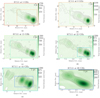 |
Fig. 1. Total intensity images of 3C 111 for the May 8, 2014, observation produced in natural weighting. In each panel the restoring beam is plotted as a white ellipse in the bottom left corner and a size scale reference of 1 pc is plotted in the top right corner. Starting from Fig. 1a, in each image, there is a colored box representing the size of the following frequency image. The frequencies are color-coded from the lowest (5 GHz) to the highest (87.6 GHz), going from red to blue. (a) 3C 111 total intensity image at 5 GHz. The beam size is 3.06 mas × 1.93 mas at −7°, the pixel size is 0.08 mas, the peak is 1.80 Jy/beam, the total intensity is 2.94 Jy, the rms is 0.21 mJy/beam, and contours are at −0.03, 0.03, 0.07, 0.18, 0.43, 1.05, 2.56, 6.23, 15.18, 36.96, 90.0% of the peak. (b) 3C 111 total intensity image at 8.4 GHz. The beam size is 1.78 mas × 1.13 mas at −11°, the pixel size is 0.04 mas, the peak is 2.28 Jy/beam, the total intensity is 3.84 Jy, the rms is 0.19 mJy/beam, and contours are at −0.04, 0.04, 0.09, 0.22, 0.52, 1.23, 2.9, 6.84, 16.15, 38.12, 90.0% of the peak. (c) 3C 111 total intensity image at 15.2 GHz. The beam size is 0.97 mas × 0.60 mas at −14°, the pixel size is 0.04 mas, the peak is 1.46 Jy/beam, the total intensity is 3.49 Jy, the rms is 0.23 mJy/beam, and contours are at −0.06, 0.06, 0.14, 0.31, 0.7, 1.57, 3.53, 7.94, 17.83, 40.06, 90.0% of the peak. (d) 3C 111 total intensity image at 21.9 GHz. The beam size is 0.79 mas × 0.51 mas at −13°, the pixel size is 0.02 mas, the peak is 1.31 Jy/beam, the total intensity is 3.33 Jy, the rms is 0.46 mJy/beam, and contours are at −0.15, 0.15, 0.3, 0.62, 1.26, 2.57, 5.23, 10.65, 21.69, 44.18, 90.0% of the peak. (e) 3C 111 total intensity image at 43.8 GHz. The beam size is 0.49 mas × 0.26 mas at −26°, the pixel size is 0.02 mas, the peak is 1.31 Jy/beam, the total intensity is 2.66 Jy, the rms is 1.14 mJy/beam, and contours are at −0.34, 0.34, 0.64, 1.18, 2.2, 4.08, 7.57, 14.06, 26.1, 48.47, 90.0% of the peak. (f) 3C 111 total intensity image at 87.6 GHz. The beam size is 0.43 mas × 0.22 mas at 77°, the pixel size is 0.02 mas, the peak is 0.89 Jy/beam, the total intensity is 1.18 Jy, the rms is 2.13 mJy/beam, and contours are at −0.84, 0.84, 1.42, 2.38, 4.0, 6.72, 11.29, 18.97, 31.88, 53.56, 90.0% of the peak. |
3.2. Core-shift analysis
The radio core is the region at the base of a jet where there is a transition from an optically thick regime to an optically thin one. Therefore, the observed position of the radio core depends on the frequency observed (e.g., Lobanov 1998). The transition region (i.e., the core) changes with frequency as r ∝ ν1/kr, where ν is the frequency and kr is the power index that, in the condition of equipartition between jet particle and magnetic field energy densities, is equal to −1. To study the core-shift, we produced and analyzed the maps in two different ways. The first method (Fits) is based on the 2D cross-correlation script FITSAlign, described in Pushkarev et al. (2012), and the second one, labeled as Modelfit, is based on the modelfit components. For the first method, we computed the equivalent beam (EB) following Eq. (2) and produced the maps with a pixel size of  . Even though Fromm et al. (2013) claimed that the best choice for the pixel size is 1/20 of the high-frequency beam size, we opted for a higher value. This was done both to avoid incurring over-resolution issues and to have comparable error bars with the Modelfit method.
where Bmin and Bmax are the minor and major axes of the restoring beam. We then produced the maps at two consecutive frequencies with the same imaging parameters (see Sect. 3.3). We chose a common pixel size of  , where CB is the common beam; that is, the mean between the two EBs. The FITSAlign script is based on the 2D pixel-based cross-correlation of a user-selected optically thin region. The program calculates a normalized cross-correlation between the low-frequency image and the selected feature of the high-frequency image using a fast method described by Lewis (1994). For each ν, we summed the obtained shift with all of the ones at higher frequencies in order to reference the core-shift values to the 87.6 GHz core. As was described in Pushkarev et al. (2012), the core shift is the offset between two maps, summed with the difference between the relative peaks in each map. Thus, after shifting the maps, we added the relative difference between the peaks, computed with Difmap. We computed the associated uncertainties for r through Eq. (3):
where x and y are the x and y position of the peak, in mas. Since Δx = Δy = px, the associated error on r is again equal to the pixel size. When summing the shifts, we propagated the uncertainties following the theory of error propagation with the help of the uncertainties2 python package. The second method is based on the modelfit components. We shifted all the modelfit components in such a way that the core component at each frequency is located at the phase center of each map. We then matched the same component at two consecutive frequencies following the procedure outlined in Sect. 4.2. We then computed the shift between the two frequencies for all the matched components. If two or more components were matched in the same frequency pair, we took the mean value for the shift. All the selected components lie in an extended region of the jet, which is optically thin.
Moreover, for every frequency, we computed the average (AVG) value between the two methods. The value of the parameters with their associated uncertainties is presented in Table 1. The two methods and their average values yield similar results for the fitting values, as can be seen in Fig. 2. The black line, r ∝ ν−1.29 ± 0.10, represents a fit of all the points. All the values from different methods are consistent with each other. The fit in the AVG case gives r ∝ ν−1.27 ± 0.17, corresponding to kr = 0.79 ± 0.17. This can be suggestive of a slight particle dominance with respect to the magnetic field energy density. We used the scipy (v1.8.0) function curve_fit to fit the parameters, taking into account the errors. The error of kr was estimated as the square root of the diagonal elements of the covariance matrix produced with the same scipy module.
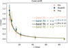 |
Fig. 2. Core-shift effect for 3C 111 between all six frequencies taken into account in this work (from 5 GHz to 87.6 GHz). The different colors represent the different methods used to estimate the core shift, as is explained in Sect. 3.2. The black line, r ∝ ν−1.29 ± 0.10, represents a fit of all the points together. The fit performed with the AVG data points gives r ∝ ν−1.27 ± 0.17, implying that kr = 0.79 ± 0.17. This result is suggestive of a mild dominance of the particle over the magnetic field, in the energy budget. |
3.3. Spectral index
We produced spectral index (Sν ∝ να) maps for all five frequency pairs to investigate the distribution of α across the jet from parsec to sub-parsec scales. The images were produced for each frequency pair, imposing the same uvmin, uvmax, mapsize, and pixelsize, and restoring beam. The relevant information is collected in Table 2 The spectral index maps were produced with the FITSAlign script (see Sect. 3.2) using a threshold of 5 × σh, where σh is the off-source rms noise of the higher-frequency map. We used Eq. (4) to estimate the uncertainties of the spectral index:
where ΔF(ν) represents the error of the flux density that was estimated following Eq. (1). The calibration contribution dominates the total error of ΔF(ν) as long as F(ν)≫σrms. This holds throughout the jet extension, whereas, on the edges of the jet, the rms contribution starts to rise. In the final spectral index images, all pixels with SNR < 5 were blanked. All the spectral index maps are presented in Fig. 3.
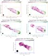 |
Fig. 3. Spectral index maps for all five frequency pairs, computed following Sect. 3.3, plotted over the higher-frequency contours. In each panel, the common beam for the two frequencies is plotted as a black circle in the bottom left corner, and a size scale reference of 1 pc is in the top right corner. The frequency pairs are color-coded from the lowest (5 − 8.4 GHz) to the highest (43.8 − 87.6 GHz), going from red to blue. The color map is chosen from a colour-vision deficiency-friendly package (Crameri 2023). |
3.4. Model-fitting of the brightness distribution
As is explained in Sect. 2, we used the modelfit function in Difmap to fit the visibilities with discrete 2D circular Gaussians. The total number of components found is 56, confirming the richness in the jet structure of 3C 111. Modelfit provides several parameters for each component: the flux density, the distance and position angle with respect to the center of the map, and the full width half maximum (FWHM) size of the Gaussian. We could then compute the observed brightness temperature, TB, and the equipartition magnetic field, Heq, for each component. The values found for all the components with the associated uncertainties are reported in Table A.1. We estimated the observed brightness temperature to be
where F(ν) is the flux density of the component in Jy, θ is its angular size in mas, ν is the observing frequency in GHz, and z is the redshift ( = 0.049) (Véron-Cetty & Véron 2006). We estimated the uncertainties for the brightness temperature with Eq. (6):
For the core component, we find observed brightness temperature values in the range 0.1 − 1.3 × 10¹² K for the various frequencies. The different range of values can be ascribed to the fact that for various resolutions, the core region can be fit with one or more modelfit components. We estimated the magnetic field under the assumption that it is at the minimum energy state (i.e., equipartition magnetic field) only for the matched components at two different frequencies (see Sect. 4.2). Therefore, it is possible to compute the magnetic flux density through Eq. (7), taken from Pacholczyk (1970):

where k is the ratio between the proton energy and the electron energy that we assumed to be 0 (i.e., purely leptonic), Φ is the filling factor that we assumed to be 13, c12 is a constant tabulated in Pacholczyk (1970) that depends on the frequencies of observations and the spectral index α, and L and V are, respectively, the luminosity and the volume of the emitting region, computed following Eq. (8).
where DL is the luminosity distance at redshift z = 0.048, obtained through Ned Wright’s cosmological calculator (Wright 2006), and is equal to ≈214 Mpc; the subscripts 1, 2 indicate, respectively, the lower and higher frequency taken into consideration; F(ν) is the flux density; and θ is the size of the modelfit component. The various components were selected following the method outlined in Sect. 4.2.
We present an image of all 56 components found through this work in Fig. 4. The position of every component was corrected for the core-shift found in Sect. 3.2. From Fig. 4, it is possible to notice that some regions of the jet can be seen and modeled at various frequencies. This leads to a recognition criterion in order to identify said Gaussian components (see Sect. 4.2).
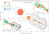 |
Fig. 4. All the modelfit components found in 3C 111, plotted over the 5 GHz contours (Fig. 1a). The components at each frequency are represented by the color in the legend, and their position is corrected for the core shift found in Sect. 3.2. The upper right panel shows the region between 9 and 2 mas in right ascension (RA) and 0 and 5 in declination (Dec). The contours are of the 21.9 GHz maps (Fig. 1d). The lower left panel shows the region between −0.5 and 3 mas in RA and −0.7 and 1.7 in Dec. The contours are of the 43.8 GHz map (Fig. 1e). |
3.5. Polarization maps
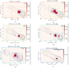 |
Fig. 5. Linear polarization intensity images of 3C 111 for the May 8, 2014, observation, plotted over the respective total intensity contours (Fig. 1). In each panel we plot the restoring beam as a white ellipse in the bottom left corner and a size scale reference of 1 pc in the top right corner. The blue bars represent the EVPAs. Starting from Fig. 5a, in each image, there is a colored box representing the size of the following frequency image. The frequencies are color-coded from the lowest (5GHz) to the highest (87.6 GHz), going from red to blue. All the information for each map can be found in Table 3. |
Total intensity and polarization data integrated over the whole structure detected in our observations.
To retrieve information on the magnetic field in the jet of 3C 111, we produced polarization maps for each frequency in the dataset. We present the polarization maps at every available frequency (Fig. 5). In the final polarization maps, all pixels with a linear polarization of ml < 9σrms, pol were blanked. We computed ml both by integrating over the source and at the polarization peak, ml, peak. All the information is presented in Table 3. By looking at the total polarized flux of 3C 111 at the highest frequency, it is possible to notice that this value is lower than the peak of the map. This is due to the different units and the fact that at 87.6 GHz the region that has a polarization above the threshold is smaller than the beam size.
3.6. Rotation measure analysis
When linearly polarized radiation crosses a magnetized medium with free electrons, the polarization angle, χ (i.e., the EVPA), rotates from its intrinsic value, χ0, following Eq. (9) via a process called birefringence (see Beck 2015, for a more complete review):

where λ is the wavelength and RM is the rotation measure. This is defined as Eq. (10):
where ne is the electron density, H∥ is the magnetic field component of the intervening medium along the line of sight, and d is the distance between the source and the observer. The rotation may occur both internally to the radio-emitting region and externally, as long as a magnetized plasma is crossed by the polarized radiation anywhere along the line of sight. By correcting the EVPAs for the effect of RM, it is also possible to study the intrinsic plane-of-sky or perpendicular electromagnetic field structure within the jet. To produce the RM maps, we combined two different sets of frequency triplets: 5 − 8.4 − 15.2 GHz (Fig. 7a) and 15.2 − 21.9 − 43.8 GHz (Fig. 7b). Both maps were produced by first convolving the images at the three different frequencies with a common circular restoring beam of diameter 1.1 mas for the lower-frequency triplets and 0.4 mas for the higher-frequency ones. The images were then aligned with a cross-correlation script following an approach similar to Sect. 3.3. To account for phase wrapping, we applied a correction to the EVPAs, making them flip by 180° if their value combined with the respective error is > 90° or < − 90°. We used the method of circular statistics outlined in Sarala & Jain (2001), which fits RM independently of the initial EVPA of the polarized emission. To account for the nπ ambiguity introduced by having a small number of frequencies for which to determine RM, we solved for nπ wraps of each EVPA, limiting our search for RM up to  . We applied the fitting function to each pixel with a linear polarization and Stokes I signal-to-noise ratio above 3σ and rejected any fits for which χ2 did not meet our significance threshold of 95% (i.e., χ2 > 3.84), as was done by Hovatta et al. (2012). As Beuchert et al. (2013) showed, for 3C111, the polarized emission at 5 GHz and 8.4 GHz can be ascribed to the core and the inner jet emission. Therefore, the integrated value of the EVPA can be used to calibrate the VLBA maps. We can thus infer various insights from the 5 − 8.4 − 15.2 GHz map (Fig. 7a). The region for which we manage to compute the RM lies at ≈6 pc from the core. The 15.2 − 21.9 − 43.8 GHz polarization images are sensitive to the inner portion of the jet, out to about 3 mas ( ≈ 3 pc) from the core. This allows us to study the RM distribution close to the central engine (Fig. 7b). The interpretation of these results is discussed in Sect. 4.3.
4. Discussion
In this section, we consider the various parameters measured in the previous one and search for correlations with the jet structure.
4.1. Spectral index distribution
The spectral index analysis performed in Sect. 3.3 can provide us with various insights into the electron population in the jet. By looking at the spectral index distribution, we can infer that the jet base is optically thick (α > 0) at all frequencies, becoming closer to a flat distribution (α = 0) as the frequency rises. The jet emission stays optically thin throughout all frequencies, reaching values of ≈ − 3 in the 43.8 − 87.6 GHz map. The general α distribution is typical of AGN jets, and is related to the optical depth of the emitting region (see Urry & Padovani 1995, for a complete review). Nonetheless, if we explore the spectral distribution in detail, we can find some discrepancies. The jet shows some optically thick features at its edges in the three lowest frequency pairs. This can be explained by considering the low SNR and, consequently, the higher errors that are present at the edge of the jet brightness distribution. If we analyze the spectral index in the region at ≈6 pc from the center of the map, we can see a clear steepening in the value of α going from −0.5 in the 5 − 8.4 GHz map to −2.5 in the 15.2 − 21.9 GHz map. If intrinsic, this can be ascribed to multiple effects like radiative losses or multiple electron distributions in that region. The same effect has been found in other objects like M87 (Nikonov et al. 2023) or NGC 315 (Ricci et al. 2022). A peculiar feature, which shows an inverted or flat distribution of α at all the frequency pairs but the highest one, is the one at ≈1.5 mas in RA and ≈0.5 mas in Dec. An inverted or flat spectrum in a region at ≈1.5 pc from the SMBH does not have a unique interpretation but it could be associated with an external electron-dense region responsible for free–free absorption (see also Sect. 4.4).
4.2. Modelfit components relations
In this section, we present an analysis of the physical quantities derived for the various components listed in Table A.1. As can be seen from Eq. (8), we require components to be matched between multiple frequencies to determine L and V. We matched components across different frequencies based on their size, θ, position angle, and relative distance to the core, r (corrected for the core-shift effect), with the following conditions:
Here, the subscript 1 indicates the component at the lower frequency and the subscript 2 indicates the component at the higher one. We retrieved a total of 22 components matched across at least two frequencies, as can be seen in Table 4.
For these components, we then investigated the interplay between the equipartition magnetic field, Heq, and the average value of different physical parameters. We notice that at the highest frequency pair (e.g., 87.6 − 43.8 GHz), the core component passes our criteria because the difference in resolution is smaller than our threshold. We acknowledge this, and we interpret the result accordingly. In Fig. 6, we show the equipartition magnetic field, Heq, as a function of the distance from the core, r. The magnetic field decreases as a function of distance with different trends based on the jet geometry (e.g., Boccardi et al. 2021; Ricci et al. 2022; Kovalev et al. 2020). The volume of the emitting region increases at larger r, while the flux density decreases, causing Heq to decrease with distance (Eq. (7)).
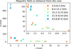 |
Fig. 6. Equipartition magnetic field, Heq, in mG vs. the distance from the core component, r, in mas. The error bars represent the uncertainties, and the arrows represent the upper or lower limits. The various colors represent the different pairs of frequencies at which each component has been matched (Sect. 4.2), as can be seen from the legend. The inset represents a zoomed-in version of the plot. |
4.3. Polarized emission and rotation measure distribution
As is described in Sect. 3.5, 3C 111 shows polarized emission at all frequencies during the observation taken into account in this paper. The polarized emission lies mostly in the jet at all frequencies, reaching its maximum value integrated over the whole emitting region at 43.8 GHz of ≈59 mJy, corresponding to a polarization degree of ≈2%, integrated over the whole emitting region. As the wavelength decreases, this emission also arises from regions progressively closer to the jet base. At 87.6 GHz (Fig. 5f), we manage to also retrieve polarized emission from the core, with an integrated value over the whole emission region of ≈5 mJy. By looking at Fig. 5, it is possible to recognize some features that are common at more than one frequency. For example, the polarized emission that arises at 43.8 GHz around 2 pc from the core (Fig. 5e can also be found in the lower frequency maps (e.g., Fig. 5c) with various intensities. In Fig. 5b, we retrieve a polarization distribution similar to the one found in Beuchert et al. (2018) in the stacked images at 15.2 GHz. They found polarization in a smaller region slightly closer to the core. Nonetheless, the EVPAs orientation is consistent with what they interpret as a continuously expanding and recollimating flow, supporting this scenario (see Beuchert et al. 2018, for more details).
The combination of polarized emission at different frequencies allows us to study the RM distribution in different jet regions, as is seen in Fig. 7. We notice that the high values of RM are caused by the innermost jet emission, which is more likely to have leakages between the Stokes parameter, low polarization signal-to-noise, and which also has χ2 values close to our threshold (3.84). Therefore, we treat such regions as artifacts. As can be seen in Fig. 7a, there seems to be a transversal gradient of RM across the jet structure, going from about −400 rad/m2 in the northern region to about 350 rad/m2 on the southern limb. The transition region between positive and negative values of RM appears to lie in the spine of the jet. In Fig. 8, we show the 33 slices that pass the criteria (with length ranging between 2 and 2.3 × θbeam) corresponding to a region with an angular size of 1.32 × 2.2 mas2, confirming the significance of the spatial size of the gradient. The median value of the maximum difference in RM values across the transversal region is  . Such a significant RM transversal gradient is strong evidence for the presence of a helical magnetic field in the jet region.
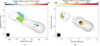 |
Fig. 7. (a): RM map between 5 GHz, 8.4 GHz, and 15.2 GHz, plotted over the 15.2 GHz contours. The green bars correspond to the Faraday-corrected EVPAs. The RM values are high because of the innermost region, which likely yields more errors due to leakage or low polarization signal-to-noise. Moreover, this region has χ2 values close to our threshold, i.e., 3.84. (b): RM map between 15.2 GHz, 21.9 GHz, and 43.8GHz, plotted over the 43.8 GHz contours. The green bars correspond to the Faraday-corrected EVPAs. |
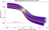 |
Fig. 8. Transversal slices of RM in the 5 − 8.4 − 15.2 GHz map (Fig. 7a) that are statistically significant (i.e., > 2θbeam) (see Hovatta et al. 2012, for details). The total number of slices is 33, each plotted with its relative error in purple. For reference, the beam size is plotted in the bottom left corner. The 33 slices occupy a region of 1.32 × 2.2 mas2. |
The magnetic field orientation is tilted by ≈ ± 45° with respect to the jet axis in the northern and southern limbs, while it is parallel to the jet axis in the spine region. This distribution is in agreement with the simulated behavior of a helical magnetic field, as was predicted by Fuentes et al. (2021). In Fig. 7b, two regions can be seen: the brightest is at about 1 mas and shows RM values from ≈3900 to ≈8500 rad/m2. It is in between the two brightest components, visible in the total intensity emission. The magnetic field orientation is almost perpendicular to the jet axis in the outer part, and it is titled to ≈60° with the jet axes in the inner part. At a distance of about 3 mas, there is an additional region with RM values ≈5000 rad/m2. Here, the magnetic field seems to be perpendicular to the jet axis.
4.4. A possible denser region at ≈1.5 pc from the SMBH
From Fig. 3, it is possible to notice that at ≈1.5pc from the central engine, there is a region with a flat or inverted spectral index. In addition to that, the RM map between 15.2 − 21.9 − 43.8 GHz (Fig. 7a) shows a positive gradient going towards this region, possibly suggesting higher values of Faraday rotation. These two independent results are consistent with the presence of a region with high free electron density and/or strong magnetic fields. By using the virial relation Eq. (12), it is possible to estimate the size of the broad-line region (RBLR):
where MBH = 108.6 M⊙ is the black hole mass taken from Chatterjee et al. (2011), G = 4.3 × 10⁻³ pc M⊙−1 (km/s)2 is the gravitational constant, f is the virial factor, estimated with Eq. 6 in Yu et al. (2019), and ΔV = 4800 km/s is the FWHM of the Hα taken from Eracleous & Halpern (2003). From this estimate, the size of the BLR is ≈0.08 pc, more than an order of magnitude smaller than the distance at which we observe a possible region with increased electron density. We therefore suggest the possibility that a cloud of the clumpy torus, which is thought to extend at ≈2 pc from the BH (Cackett et al. 2021), is responsible for what we observe, since it can explain both the flat or inverted spectrum at higher frequencies in a region different from the core and the high values of RM.
5. Conclusion
In this paper, we present a set of multifrequency, high-angular-resolution observations of parsec-scale radio emission in the BLRG 3C 111. The images were obtained in full polarization with the VLBA, and as such our work is the first study of this jet with simultaneous data from 5 GHz up to 87.6 GHz. In the highest-angular-resolution image (87.6 GHz), our convolving beam is as small as 0.22 mas, corresponding to ≈0.2 pc. The source is well detected at all frequencies, dominated by a compact core of brightness ranging between ≈3 Jy and ≈1 Jy (at 8.4 GHz and 87.6 GHz, respectively). Our main results can be summarized as follows:
-
From the core, a one-sided jet emerges, extending up to ≈25 mas in length at 5 GHz. The jet is remarkably straight, being oriented at a position angle of ≈65° and showing little to no evidence of bending over its full extension. Thanks to the multifrequency analysis, it was possible to perform the core-shift analysis, in which we found a trend of r ∝ ν−1.27 ± 0.17, implying that kr = 0.79 ± 0.17. This is suggestive of a slight dominance of the particle energy density with respect to the magnetic field.
-
We computed the spectral index maps of the source. For the core, the spectral index varies from α ≈ 1.5 in the lower-frequency pair, 5 − 8.4 GHz, to α ≈ 0 in the higher-frequency pair, 43.8 − 87.6 GHz. The spectral index along the jet is generally steep, reaching the minimum value of α ≈ −3 in the highest-frequency pair. When the same jet region is detected in more than one frequency pair, its spectral index steepens at a higher frequency. This could be due to different effects, such as radiative losses or multilayer electron distribution, as it is found in other AGN (e.g., Nikonov et al. 2023; Ricci et al. 2022).
-
From our model-fitting analysis, we found 56 components across all frequencies. We then estimated the brightness temperature distribution across the source for all the components. We found values in the range of 107 − 1012 K. Under the assumption that the emitting region is at the minimum total energy, the equipartition magnetic field was estimated for those components that we matched at different frequencies. We found values in the range of 1 − 100 mG.
-
The polarized emission lies mostly in the jet at all the frequencies and, with increasing frequency, this emission also arises from regions progressively closer to the jet base. The integrated fraction of polarization spans from a minimum of 0.40% at 87.6 GHz, where only the core shows polarized emission, to 2.21% at 43.8 GHz. Our results confirm the scenario proposed by Beuchert et al. (2018) of an interaction of traveling features with a standing shock downstream in the jet.
-
By considering the polarized regions common to various frequencies, we computed the RM for two triplets of frequencies. For the 15.2 − 21.9 − 43.8 GHz triplet, we identified two regions: the brightest one is at ≈2 pc from the core and shows a gradient of RM from ≈3900 to ≈8400 rad/m2; at a distance of about 3 mas, there lies another region with RM values of ≈6000 rad/m2. In this outer region, the magnetic field seems to start aligning with the jet axis. At the lowest frequencies, the region with common polarised emission is at a distance of ≈6 mas from the core. In this region, there is a significant transverse gradient of RM, going from about 250 rad/m2 down to ≈ − 400 rad/m2. The magnetic field orientation is perpendicular to the jet axis in the central region, where the transition from positive to negative values of RM happens. In the outer region, the magnetic field seems to align with the jet axis. This magnetic field distribution is in agreement with a helical structure (Fuentes et al. 2021).
-
By looking at the spectral index map between 21.9 GHz and 43.8 GHz and the RM between 15.2 − 21.9 − 43.8 GHz, there seems to be a co-spatiality between the region of the flat or inverted spectrum and the region with a high RM value. We propose, as a possible explanation, a cloud of the clumpy torus that lies at ≈1.5 pc from the SMBH.
Acknowledgments
We would like to thank Dr. M. Kadler and Dr. B. Boccardi for their helpful discussion, which improved the manuscript. This paper made use of “Uncertainties: a Python package for calculations with uncertainties, Eric O. LEBIGOT”, http://pythonhosted.org/uncertainties/. This research has made use of data from the MOJAVE database that is maintained by the MOJAVE team (Lister et al. 2018). This research has been partially funded by the Deutsche Forschungsgemeinschaft (DFG, German Research Foundation) – project number 443220636 (DFG research unit FOR 5195: “Relativistic Jets in Active Galaxies”). J.D.L. would like to acknowledge that this publication is part of the M2FINDERS project, which has received funding from the European Research Council (ERC) under the European Union’s Horizon 2020 Research and Innovation Programme (grant agreement No 101018682).
References
- Angelakis, E., Fuhrmann, L., Myserlis, I., et al. 2019, A&A, 626, A60 [NASA ADS] [CrossRef] [EDP Sciences] [Google Scholar]
- Beck, R. 2015, A&ARv, 24, 4 [Google Scholar]
- Bennett, C. L., Larson, D., Weiland, J. L., & Hinshaw, G. 2014, ApJ, 794, 135 [Google Scholar]
- Beuchert, T., Kadler, M., Wilms, J., et al. 2013, Eur. Phys. J. Web Conf., 61, 06006 [Google Scholar]
- Beuchert, T., Kadler, M., Perucho, M., et al. 2018, A&A, 610, A32 [NASA ADS] [CrossRef] [EDP Sciences] [Google Scholar]
- Boccardi, B., Perucho, M., Casadio, C., et al. 2021, A&A, 647, A67 [NASA ADS] [CrossRef] [EDP Sciences] [Google Scholar]
- Cackett, E. M., Bentz, M. C., & Kara, E. 2021, iScience, 24, 102557 [NASA ADS] [CrossRef] [Google Scholar]
- Casadio, C., Gómez, J. L., Grandi, P., et al. 2015, ApJ, 808, 162 [Google Scholar]
- Casadio, C., Marscher, A. P., Jorstad, S. G., et al. 2019, A&A, 622, A158 [NASA ADS] [CrossRef] [EDP Sciences] [Google Scholar]
- Chatterjee, R., Marscher, A. P., Jorstad, S. G., et al. 2011, ApJ, 734, 43 [NASA ADS] [CrossRef] [Google Scholar]
- Crameri, F. 2023, https://doi.org/10.5281/zenodo.8035877 [Google Scholar]
- Eracleous, M., & Halpern, J. P. 2003, ApJ, 599, 886 [NASA ADS] [CrossRef] [Google Scholar]
- Event Horizon Telescope Collaboration (Akiyama, K., et al.) 2019, ApJ, 875, L1 [Google Scholar]
- Fanaroff, B. L., & Riley, J. M. 1974, MNRAS, 167, 31 [Google Scholar]
- Fichet de Clairfontaine, G., Meliani, Z., & Zech, A. 2022, A&A, 661, A54 [NASA ADS] [CrossRef] [EDP Sciences] [Google Scholar]
- Fromm, C. M., Ros, E., Perucho, M., et al. 2013, A&A, 557, A105 [NASA ADS] [CrossRef] [EDP Sciences] [Google Scholar]
- Fuentes, A., Torregrosa, I., Martí, J. M., Gómez, J. L., & Perucho, M. 2021, A&A, 650, A61 [NASA ADS] [CrossRef] [EDP Sciences] [Google Scholar]
- Grandi, P., Torresi, E., & Stanghellini, C. 2012, ApJ, 751, L3 [NASA ADS] [CrossRef] [Google Scholar]
- Greisen, E. W. 2003, in Information Handling in Astronomy - Historical Vistas, ed. A. Heck, Astrophysics and Space Science Library, 285,109 [NASA ADS] [CrossRef] [Google Scholar]
- Högbom, J. A. 1974, A&AS, 15, 417 [Google Scholar]
- Homan, D. C., Ojha, R., Wardle, J. F. C., et al. 2002, ApJ, 568, 99 [NASA ADS] [CrossRef] [Google Scholar]
- Hovatta, T., Lister, M. L., Aller, M. F., et al. 2012, AJ, 144, 105 [Google Scholar]
- Jorstad, S. G., Marscher, A. P., Lister, M. L., et al. 2005, AJ, 130, 1418 [Google Scholar]
- Jorstad, S. G., Marscher, A. P., Morozova, D. A., et al. 2017, ApJ, 846, 98 [Google Scholar]
- Kadler, M., Ros, E., Perucho, M., et al. 2008, ApJ, 680, 867 [NASA ADS] [CrossRef] [Google Scholar]
- Kettenis, M., van Langevelde, H. J., Reynolds, C., & Cotton, B. 2006, in Astronomical Data Analysis Software and Systems XV, eds. C. Gabriel, C. Arviset, D. Ponz, & S. Enrique, ASP Conf. Ser., 351, 497 [NASA ADS] [Google Scholar]
- Kovalev, Y. Y., Pushkarev, A. B., Nokhrina, E. E., et al. 2020, MNRAS, 495, 3576 [NASA ADS] [CrossRef] [Google Scholar]
- Lewis, J. 1994, Vis. Interface, 95 [Google Scholar]
- Lico, R., Giroletti, M., Orienti, M., et al. 2012, A&A, 545, A117 [CrossRef] [EDP Sciences] [Google Scholar]
- Linfield, R., & Perley, R. 1984, ApJ, 279, 60 [Google Scholar]
- Lister, M. L., Cohen, M. H., Homan, D. C., et al. 2009, AJ, 138, 1874 [NASA ADS] [CrossRef] [Google Scholar]
- Lister, M. L., Aller, M. F., Aller, H. D., et al. 2018, ApJS, 234, 12 [CrossRef] [Google Scholar]
- Lobanov, A. P. 1998, A&A, 330, 79 [NASA ADS] [Google Scholar]
- Nikonov, A. S., Kovalev, Y. Y., Kravchenko, E. V., Pashchenko, I. N., & Lobanov, A. P. 2023, MNRAS, 526, 5949 [NASA ADS] [CrossRef] [Google Scholar]
- Orienti, M., Venturi, T., Dallacasa, D., et al. 2011, MNRAS, 417, 359 [NASA ADS] [CrossRef] [Google Scholar]
- Pacholczyk, A. G. 1970, Radio astrophysics. Nonthermal processes in galactic and extragalactic sources (San Francisco: WH Freeman and Co.) [Google Scholar]
- Perucho, M. 2019, Galaxies, 7, 70 [Google Scholar]
- Perucho, M., Agudo, I., Gómez, J. L., et al. 2008, A&A, 489, L29 [NASA ADS] [CrossRef] [EDP Sciences] [Google Scholar]
- Pushkarev, A. B., Hovatta, T., Kovalev, Y. Y., et al. 2012, A&A, 545, A113 [NASA ADS] [CrossRef] [EDP Sciences] [Google Scholar]
- Ricci, L., Boccardi, B., Nokhrina, E., et al. 2022, A&A, 664, A166 [NASA ADS] [CrossRef] [EDP Sciences] [Google Scholar]
- Sarala, S., & Jain, P. 2001, MNRAS, 328, 623 [NASA ADS] [CrossRef] [Google Scholar]
- Schulz, R., Kadler, M., Ros, E., et al. 2020, A&A, 644, A85 [NASA ADS] [CrossRef] [EDP Sciences] [Google Scholar]
- Shepherd, M. C. 1997, in Astronomical Data Analysis Software and Systems VI, eds. G. Hunt, & H. Payne, ASP Conf. Ser., 125, 77 [Google Scholar]
- Urry, C. M., & Padovani, P. 1995, PASP, 107, 803 [NASA ADS] [CrossRef] [Google Scholar]
- Véron-Cetty, M. P., & Véron, P. 2006, A&A, 455, 773 [Google Scholar]
- Wright, E. L. 2006, PASP, 118, 1711 [NASA ADS] [CrossRef] [Google Scholar]
- Yu, L.-M., Bian, W.-H., Wang, C., Zhao, B.-X., & Ge, X. 2019, MNRAS, 488, 1519 [Google Scholar]
Appendix A: modelfit components
All 56 modelfit components parameters with respective uncertainties (see Sect. 3.4).
All Tables
Total intensity and polarization data integrated over the whole structure detected in our observations.
All 56 modelfit components parameters with respective uncertainties (see Sect. 3.4).
All Figures
|
Fig. 1. Total intensity images of 3C 111 for the May 8, 2014, observation produced in natural weighting. In each panel the restoring beam is plotted as a white ellipse in the bottom left corner and a size scale reference of 1 pc is plotted in the top right corner. Starting from Fig. 1a, in each image, there is a colored box representing the size of the following frequency image. The frequencies are color-coded from the lowest (5 GHz) to the highest (87.6 GHz), going from red to blue. (a) 3C 111 total intensity image at 5 GHz. The beam size is 3.06 mas × 1.93 mas at −7°, the pixel size is 0.08 mas, the peak is 1.80 Jy/beam, the total intensity is 2.94 Jy, the rms is 0.21 mJy/beam, and contours are at −0.03, 0.03, 0.07, 0.18, 0.43, 1.05, 2.56, 6.23, 15.18, 36.96, 90.0% of the peak. (b) 3C 111 total intensity image at 8.4 GHz. The beam size is 1.78 mas × 1.13 mas at −11°, the pixel size is 0.04 mas, the peak is 2.28 Jy/beam, the total intensity is 3.84 Jy, the rms is 0.19 mJy/beam, and contours are at −0.04, 0.04, 0.09, 0.22, 0.52, 1.23, 2.9, 6.84, 16.15, 38.12, 90.0% of the peak. (c) 3C 111 total intensity image at 15.2 GHz. The beam size is 0.97 mas × 0.60 mas at −14°, the pixel size is 0.04 mas, the peak is 1.46 Jy/beam, the total intensity is 3.49 Jy, the rms is 0.23 mJy/beam, and contours are at −0.06, 0.06, 0.14, 0.31, 0.7, 1.57, 3.53, 7.94, 17.83, 40.06, 90.0% of the peak. (d) 3C 111 total intensity image at 21.9 GHz. The beam size is 0.79 mas × 0.51 mas at −13°, the pixel size is 0.02 mas, the peak is 1.31 Jy/beam, the total intensity is 3.33 Jy, the rms is 0.46 mJy/beam, and contours are at −0.15, 0.15, 0.3, 0.62, 1.26, 2.57, 5.23, 10.65, 21.69, 44.18, 90.0% of the peak. (e) 3C 111 total intensity image at 43.8 GHz. The beam size is 0.49 mas × 0.26 mas at −26°, the pixel size is 0.02 mas, the peak is 1.31 Jy/beam, the total intensity is 2.66 Jy, the rms is 1.14 mJy/beam, and contours are at −0.34, 0.34, 0.64, 1.18, 2.2, 4.08, 7.57, 14.06, 26.1, 48.47, 90.0% of the peak. (f) 3C 111 total intensity image at 87.6 GHz. The beam size is 0.43 mas × 0.22 mas at 77°, the pixel size is 0.02 mas, the peak is 0.89 Jy/beam, the total intensity is 1.18 Jy, the rms is 2.13 mJy/beam, and contours are at −0.84, 0.84, 1.42, 2.38, 4.0, 6.72, 11.29, 18.97, 31.88, 53.56, 90.0% of the peak. |
| In the text | |
|
Fig. 2. Core-shift effect for 3C 111 between all six frequencies taken into account in this work (from 5 GHz to 87.6 GHz). The different colors represent the different methods used to estimate the core shift, as is explained in Sect. 3.2. The black line, r ∝ ν−1.29 ± 0.10, represents a fit of all the points together. The fit performed with the AVG data points gives r ∝ ν−1.27 ± 0.17, implying that kr = 0.79 ± 0.17. This result is suggestive of a mild dominance of the particle over the magnetic field, in the energy budget. |
| In the text | |
|
Fig. 3. Spectral index maps for all five frequency pairs, computed following Sect. 3.3, plotted over the higher-frequency contours. In each panel, the common beam for the two frequencies is plotted as a black circle in the bottom left corner, and a size scale reference of 1 pc is in the top right corner. The frequency pairs are color-coded from the lowest (5 − 8.4 GHz) to the highest (43.8 − 87.6 GHz), going from red to blue. The color map is chosen from a colour-vision deficiency-friendly package (Crameri 2023). |
| In the text | |
|
Fig. 4. All the modelfit components found in 3C 111, plotted over the 5 GHz contours (Fig. 1a). The components at each frequency are represented by the color in the legend, and their position is corrected for the core shift found in Sect. 3.2. The upper right panel shows the region between 9 and 2 mas in right ascension (RA) and 0 and 5 in declination (Dec). The contours are of the 21.9 GHz maps (Fig. 1d). The lower left panel shows the region between −0.5 and 3 mas in RA and −0.7 and 1.7 in Dec. The contours are of the 43.8 GHz map (Fig. 1e). |
| In the text | |
|
Fig. 5. Linear polarization intensity images of 3C 111 for the May 8, 2014, observation, plotted over the respective total intensity contours (Fig. 1). In each panel we plot the restoring beam as a white ellipse in the bottom left corner and a size scale reference of 1 pc in the top right corner. The blue bars represent the EVPAs. Starting from Fig. 5a, in each image, there is a colored box representing the size of the following frequency image. The frequencies are color-coded from the lowest (5GHz) to the highest (87.6 GHz), going from red to blue. All the information for each map can be found in Table 3. |
| In the text | |
|
Fig. 6. Equipartition magnetic field, Heq, in mG vs. the distance from the core component, r, in mas. The error bars represent the uncertainties, and the arrows represent the upper or lower limits. The various colors represent the different pairs of frequencies at which each component has been matched (Sect. 4.2), as can be seen from the legend. The inset represents a zoomed-in version of the plot. |
| In the text | |
|
Fig. 7. (a): RM map between 5 GHz, 8.4 GHz, and 15.2 GHz, plotted over the 15.2 GHz contours. The green bars correspond to the Faraday-corrected EVPAs. The RM values are high because of the innermost region, which likely yields more errors due to leakage or low polarization signal-to-noise. Moreover, this region has χ2 values close to our threshold, i.e., 3.84. (b): RM map between 15.2 GHz, 21.9 GHz, and 43.8GHz, plotted over the 43.8 GHz contours. The green bars correspond to the Faraday-corrected EVPAs. |
| In the text | |
|
Fig. 8. Transversal slices of RM in the 5 − 8.4 − 15.2 GHz map (Fig. 7a) that are statistically significant (i.e., > 2θbeam) (see Hovatta et al. 2012, for details). The total number of slices is 33, each plotted with its relative error in purple. For reference, the beam size is plotted in the bottom left corner. The 33 slices occupy a region of 1.32 × 2.2 mas2. |
| In the text | |
Current usage metrics show cumulative count of Article Views (full-text article views including HTML views, PDF and ePub downloads, according to the available data) and Abstracts Views on Vision4Press platform.
Data correspond to usage on the plateform after 2015. The current usage metrics is available 48-96 hours after online publication and is updated daily on week days.
Initial download of the metrics may take a while.