| Issue |
A&A
Volume 697, May 2025
|
|
|---|---|---|
| Article Number | A106 | |
| Number of page(s) | 17 | |
| Section | Numerical methods and codes | |
| DOI | https://doi.org/10.1051/0004-6361/202553886 | |
| Published online | 14 May 2025 | |
An efficient integrator for stellar dynamics in effective gravity fields based on the isochrone potential
LTE, Observatoire de Paris, Université PSL, Sorbonne Université, Université de Lille, LNE, CNRS,
61 Avenue de l’Observatoire,
75014
Paris,
France
★ Corresponding author: This email address is being protected from spambots. You need JavaScript enabled to view it.
Received:
24
January
2025
Accepted:
19
March
2025
Abstract
Context. Integrating the motion of stars immersed in some smoothed potential is necessary in many stellar and galactic studies. Previous works have generally used numerical integrators that alternate between linear drifts and velocity kicks (such as the standard Leapfrog scheme). The low efficiency of this approach contrasts with the sophisticated methods developed in other fields such as planetary dynamics, for which integrators alternate between Keplerian drifts and velocity kicks.
Aims. Inspired by the splitting methods used in planetary dynamics, we aim to build an efficient integration scheme dedicated to stellar and galactic dynamics.
Methods. We took advantage of the peculiar properties of Hénon’s isochrone potential to design a new symplectic splitting scheme that can be used to integrate the motion of stars in any gravitational potential. This scheme alternates between isochrone drifts and velocity kicks. As a first application, we considered the motion of a star in a Plummer potential – an essential constituent of galactic potentials – and determined the set of integration parameters that provide the best integration efficiency (i.e. the best conservation of total energy for the lowest computational cost).
Results. We derived the analytical solution for all possible kinds of orbits in Hénon’s isochrone potential (bound and unbound trajectories) as needed in our integration scheme. Our numerical experiments for stars in a Plummer potential show excellent performances in regions in the inner and outer parts of the gravity field, that is, where the motion of stars is well approximated by isochrone trajectories (with perturbations of order 10−3 or less). For highly elongated orbits that cross the characteristic length of the Plummer potential, the performance is equivalent to that of previous methods.
Conclusions. The splitting scheme presented here is a good alternative to previous methods: it performs at least as well, and up to orders of magnitude better, depending on the dynamical regime of the star.
Key words: methods: analytical / methods: numerical / stars: kinematics and dynamics / galaxies: kinematics and dynamics
© The Authors 2025
 Open Access article, published by EDP Sciences, under the terms of the Creative Commons Attribution License (https://creativecommons.org/licenses/by/4.0), which permits unrestricted use, distribution, and reproduction in any medium, provided the original work is properly cited.
This article is published in open access under the Subscribe to Open model. This email address is being protected from spambots. You need JavaScript enabled to view it. to support open access publication.
1 Introduction
Numerical integration of gravitational systems is a crucial component in solving many astrophysics problems. According to Pouliasis et al. (2017), ‘The study of the orbits of stars and stellar systems, like globular and open clusters in the Milky Way, is essential to understand the properties of the different Galactic stellar populations (thin and thick discs, stellar halo) and their mode of formation’. For instance, Khoperskov et al. (2020) propose a dynamical explanation for the presence of metal-rich stars in the outer Galactic disc. But this is not the only relevant context: for example, the galactic influences to which trans-Neptunian objects in the Oort Cloud have been subjected since the formation of the Solar System – like passing stars or galactic tides (see Saillenfest 2020, for a review) – depend on the trajectory of the Sun within the Milky Way (Kaib et al. 2011; Martínez-Barbosa et al. 2017). The Sun’s motion through the Milky Way may also be correlated with geological cyclic sedimentation over long timescales (Boulila et al. 2018). These examples, though not exhaustive, underscore the importance of integrating the trajectories of stars within the Galaxy.
In stellar dynamics, the large number of particles makes numerical resolution extremely demanding in terms of computational performance. Fortunately, in relatively dilute regimes such as galaxies, the gravitational force acting on a star can be approximated as arising from a smooth density distribution rather than a discrete collection of mass points (Binney & Tremaine 2008). At the same time, the exact form of the galactic potential remains unknown and is the subject of active research (see e.g. the discussions by Pouliasis et al. 2017). As such, ‘the study of individual orbits in various galactic potentials is an important branch of galactic dynamics’ (Greiner 1987). Depending on the model used and the initial conditions, orbits can change significantly (see e.g. Pichardo et al. 2004; Zotos 2014; Caritá et al. 2018). Therefore, the exploration of possible trajectories often requires sampling thousands of initial conditions and integrating them all numerically over long timescales, as done for instance by Martínez-Barbosa et al. (2017). For this purpose, the numerical integrator used must be fast and reliable, that is, it must show good stability properties over long timescales.
For planetary systems, much effort has been put into designing integrators that optimise computational cost while preserving the symplectic structure of the Hamiltonian (see e.g. Wisdom & Holman 1991; Chambers 1999; Laskar & Robutel 2001; Farrés et al. 2013; Rein & Tamayo 2015; Rein et al. 2019; Hernandez & Dehnen 2024). These integrators take advantage of the specific properties of planetary systems – or any system with a similar hierarchy – that are made of a dominant central mass (the ‘star’) and other, much smaller bodies (the ‘planets’), such that most orbits follow perturbed Keplerian ellipses. These integrators therefore alternate between Keplerian drifts and velocity corrections. We refer to this methodology as ‘Kepler splitting’. Kepler splitting has shown its merits not only in the context of interacting planets (serial problem), but also for non-interacting test particles affected by known – or pre-computed – perturbations (the parallel problem, e.g. small moons, asteroids, and comets). By allowing people to use much larger time steps, computation costs are dramatically reduced.
To our knowledge, no dedicated integrators have been designed for the dynamics of stars immersed in effective galactic potentials, even though stellar orbits do exhibit some remarkable properties. The widely used galpy Python package (Bovy 2015) provides a handful of symplectic integrators, which include a second-order scheme (also known as ‘Leapfrog’), the fourth-order scheme from Forest & Ruth (1990), and the sixth-order scheme from Yoshida (1990)1. These schemes are multi-purpose integrators in the sense that they do not take advantage of any specific property of stellar trajectories. Their principle is to alternate between linear drifts and velocity kicks – implicitly assuming that the trajectories followed are perturbed rectilinear motions. We refer to this method as ‘kinetic splitting’.
Besides the limitations of kinetic splitting, the fourth- and sixth-order schemes implemented in galpy include large negative sub-steps, which results in ‘not very good stability properties for large step sizes’ (Laskar & Robutel 2001, Sect. 1, paragraph 1; see also the discussions by Blanes et al. 2013 and Farrés et al. 2013). As a result, ‘[there are regimes where], at an equivalent cost, the leapfrog integrators become more effective’ (Laskar & Robutel 2001, Sect. 3, last paragraph). Pascale et al. (2022) even conclude that in some cases, the fourth-order Runge-Kutta (RK4) method is more stable than the integrator from Forest & Ruth (1990), despite RK4 being not symplectic. This probably explains why the integrators generally used in stellar dynamics are of low order, such as the Leapfrog (see e.g. Pouliasis et al. 2017; Ferrone et al. 2023), or ‘Runge-Kutta’ (see e.g. Smirnova 2015; Boulila et al. 2018; Sharina et al. 2018; Pascale et al. 2022; Baba et al. 2024; Khalil et al. 2024). Some integrators are symplectic, while others are not2.
The choice of low-order integrators in galactic dynamics also comes from the fact that using a smoothed galactic potential is itself an approximation that neglects the effect of close encounters between stars. This approximation is good for dilute systems, such as field stars in galaxies3, but poor for dense stellar clusters in the process of relaxation. Hence, in this context, highly accurate numerical integrations are not needed: instead, general properties of stellar dynamics are computed from an ensemble of many trajectories, whose statistics do not critically depend on the accuracy of each individual orbit (see e.g. Portegies Zwart & Boekholt 2014; Hernandez et al. 2020 for N-body systems). Yet, to avoid producing biased statistics, general properties of the dynamical system must be correctly reproduced by numerical integrations – even at a reduced precision. For instance, we do not want conserved quantities (e.g. the total energy) to irreversibly drift over time away from those of the original system. To this aim, irrespective of the integrator chosen, reasonably small integration time steps must be used. When aiming for a given level of energy conservation, the question of how large the time steps can possibly be depends on the integration method – in particular, the choice of splitting.
We investigated whether we can take advantage of the very good properties of splitting symplectic integrators in the context of stellar and galactic dynamics using an appropriate splitting of the Hamiltonian function. The goal of this new splitting is to decrease computation costs, in particular when many thousands of trajectories are needed.
Contrary to planetary – or asteroid – dynamics, there is no obvious choice of splitting, because trajectories in most smoothed potentials used for galaxies (e.g. Plummer 1911) cannot be solved analytically. This contrasts with the dominant Keplerian potential found in planetary systems. However, one galactic potential does admit analytical solutions: Hénon’s isochrone potential (Hénon 1959b,a). Our idea is to use this potential as the basis of a new splitting scheme, which would alternate between isochrone drifts and velocity kicks. We call it ‘isochrone splitting’. As shown below, isochrone splitting can be seen as a generalisation of Kepler splitting. Our aim here is to use it in the context of non-collisional stellar trajectories in galactic potentials.
Even though generic galactic potentials are not isochrone, the Hénon isochrone potential does generate rosette-shaped trajectories resembling those of many stars in the plane of the Milky Way (see e.g. Dinescu et al. 1999; Pouliasis et al. 2017; Boulila et al. 2018; Pérez-Villegas et al. 2018; Ibata et al. 2019; Ferrone et al. 2023). Besides, the isochrone potential is guaranteed to be a very efficient splitting scheme when we consider the orbits of distant stars in any centrally condensed potential. This property comes from the fact that all centrally condensed potentials (including the Hénon isochrone) tend to the Kepler potential at large distances. At small radii, near the centre of the mass distribution, the isochrone potential tends to a harmonic potential, which is a property shared by most potentials used in galactic dynamics (e.g. Plummer 1911; Miyamoto & Nagai 1975, the Halo component of Paczynski 1990, etc.). These characteristics of the isochrone potential make us confident that, at least in specific regimes, the isochrone potential should offer a very good kernel for a symplectic splitting.
As a first application, we present the isochrone splitting scheme for integrating the motion of a star in a Plummer potential (Plummer 1911). Even though the Plummer potential was initially introduced to model globular clusters, it is now a fundamental building block of smoothed galactic potentials, used to compute non-collisional stellar trajectories within galaxies (see e.g. Allen & Santillan 1991 and other references in this section). The Plummer potential is generally used to model galactic bulges; for stars orbiting in the disc plane, the Miyamoto-Nagai potential used to model galactic discs also reduces to the Plummer potential (Miyamoto & Nagai 1975). The omnipresence of the Plummer potential in galactic models and its simplicity motivate its use here as a testbed for the isochrone splitting scheme.
In Sect. 2, we recall the basics of splitting symplectic integrators. In Sect. 3 we present the analytical solutions of the isochrone dynamics needed by our integration scheme. In Sect. 4 we outline how to use these analytical solutions to build a new splitting scheme. In Sect. 5, we determine how to maximise the performances of the isochrone splitting scheme in the context of a particle orbiting in a Plummer potential. In Sect. 6, we illustrate our analytical results for a star orbiting in a Plummer globular cluster and compare them to those of other integration methods. Finally, we discuss our choice of integration parameters in Sect. 7 and conclude in Sect. 8.
2 Splitting symplectic integrators
Throughout the article, we use the following symbol: dX as the total derivative operator with respect to the variable X.
2.1 Basics of symplectic integrators
Let ℋ(x) be an autonomous Hamiltonian with m degrees of freedom, where x = (q, p) ∈ ℝ2m is the state vector, with q ∈ ℝm denoting the generalised coordinates and p ∈ ℝm the conjugate momenta. The time evolution of the state vector is governed by Hamilton’s equation, which can be expressed as
![Mathematical equation: $\[\mathrm{d}_t \mathbf{x}=\{\mathbf{x}, \mathcal{H}\}=\mathcal{L}_{\mathcal{H}} \mathbf{x},\]$](/articles/aa/full_html/2025/05/aa53886-25/aa53886-25-eq1.png) (1)
(1)
where ℒℋ := {. , ℋ} is the Lie derivative4 along the flow of ℋ. The flow of ℋ is defined as the map
![Mathematical equation: $\[\phi_t^{\mathcal{H}}: \mathbf{x}_0 \mapsto \mathbf{x}(t),\]$](/articles/aa/full_html/2025/05/aa53886-25/aa53886-25-eq2.png) (2)
(2)
which associates with every point x0 in the phase space the position x of the system at time t, starting from the initial condition x0 at time t = 0. The formal solution of Eq. (1) is
![Mathematical equation: $\[\phi_t^{\mathcal{H}}\left(\mathbf{x}_0\right)=e^{t \mathcal{L}_{\mathcal{H}}} \phi_0^{\mathcal{H}}\left(\mathbf{x}_0\right).\]$](/articles/aa/full_html/2025/05/aa53886-25/aa53886-25-eq3.png) (3)
(3)
In general, analytical solutions of the equations of motion do not exist, so we need to integrate Eq. (1) numerically. In principle, any standard non-symplectic integrator can be used for this purpose (such as the methods of Euler or Runge-Kutta; see e.g. Hairer et al. 2006). However, these methods provide an approximate solution to an exact system of equations, with no guarantee that fundamental properties of the original system will be preserved – such as the conservation of energy, the time reversibility, or the area-preserving nature of the flow in the phase space. Therefore, these integrators inevitably lead, over time, to a drift in total energy5, which distorts the dynamical structure of the system. In Hamiltonian mechanics, although these types of integrators can be used, there is a way to bypass this problem by reversing the approach: instead of seeking an approximate solution to an exact system of equations, one seeks the exact solution of an approximate Hamiltonian system of equations. This type of integrator is called a symplectic integrator (see e.g. Yoshida 1993; Hairer et al. 2006 for a comprehensive review). The solution obtained tends to oscillate around the true solution, with no irreversible drift in energy away from the real system. As such, the qualitative behaviour of the system remains correct even over long-term integrations. For accurate results, however, the oscillations artificially introduced by the symplectic integration scheme need to be minimised as much as possible.
The splitting method is the simplest kind of symplectic integrator to implement: it approximates the operator etℒℋ in Eq. (3). We consider the case in which ℋ(x) can be split into two individually integrable parts:
![Mathematical equation: $\[\mathcal{H}=\mathcal{H}_{\mathrm{A}}+\mathcal{H}_{\mathrm{B}}.\]$](/articles/aa/full_html/2025/05/aa53886-25/aa53886-25-eq4.png) (4)
(4)
A symplectic splitting scheme with N steps is obtained by approximating ℋ by a Hamiltonian κ for which the flow ![Mathematical equation: $\[\phi_{\delta t}^{\mathcal{K}}\]$](/articles/aa/full_html/2025/05/aa53886-25/aa53886-25-eq5.png) is exactly given by
is exactly given by
![Mathematical equation: $\[\mathcal{S}_N=\prod_{i=1}^N e^{c_i \delta t \mathcal{L}_{\mathcal{H}_{\mathrm{A}}}} e^{d_i \delta t \mathcal{L}_{\mathcal{H}_{\mathrm{B}}}},\]$](/articles/aa/full_html/2025/05/aa53886-25/aa53886-25-eq6.png) (5)
(5)
where (ci, di) ∈ ℝ2. Therefore, performing one time step δt with Hamiltonian κ simply amounts to alternate sub-steps with the (analytical) propagation of ℋA and ℋB. Moreover, it is symmetric if
![Mathematical equation: $\[\mathcal{S}_N(\delta t) \mathcal{S}_N(-\delta t)=\mathcal{S}_N(-\delta t) \mathcal{S}_N(\delta t)=\mathbb{1},\]$](/articles/aa/full_html/2025/05/aa53886-25/aa53886-25-eq7.png) (6)
(6)
which means that it has the exact time reversibility. In this case, the Hamiltonian κ is necessarily even with respect to δt.
In practice, the coefficients ci and di are chosen such that the difference |ℋ − κ| is as small as possible. A symplectic integrator is said to be of ‘order p′ if ℋ = κ + 𝒪(δtp). For instance, the Leapfrog integration scheme,
![Mathematical equation: $\[\mathcal{S}_2=e^{\frac{\delta t}{2} \mathcal{L}_{\mathcal{H}_{\mathrm{A}}}} e^{\delta t \mathcal{L}_{\mathcal{H}_{\mathrm{B}}}} e^{\frac{\delta t}{2} \mathcal{L}_{\mathcal{H}_{\mathrm{A}}}},\]$](/articles/aa/full_html/2025/05/aa53886-25/aa53886-25-eq8.png) (7)
(7)
is a symmetric symplectic scheme of order 2.
Very efficient symplectic schemes can be obtained if the splitting of ℋ in Eq. (4) is hierarchical, that is, if we can write ℋA = 𝒜 and ℋB = εℬ, where ε ≪ 1. For instance, the symmetric integrators 𝒮𝒜ℬ𝒜n and 𝒮𝒜ℬ𝒜𝒞n of Laskar & Robutel (2001) have errors ℋ − κ = 𝒪(εδt2n) + 𝒪(ε2δt2), and 𝒪(εδt2n) + 𝒪(ε2δt4), respectively6. The fact that powers of ε appear in the remainders means that if ε is small, even a scheme with a small number of steps N gives very good performances. For instance, the integrator 𝒮𝒜ℬ𝒜3 has 4 steps and it behaves as an integrator of order 6 if ε is small enough, despite remainders being formally of order 2 in δt. For comparison, the integrator given by Forest & Ruth (1990) has the same number of steps as 𝒮𝒜ℬ𝒜3 but it is of order 4 (Laskar & Robutel 2001). More general symplectic schemes have been developed by Blanes et al. (2013), with remainders of the form ℋ − κ = 𝒪(εδts1) + 𝒪(ε2δts2) + 𝒪(ε3δts3) + ... where {s1, s2, s3 ...} are even integer coefficients. These integrators are symmetric and do not have negative coefficients ci and di; or, if they do, such coefficients are few and very small (lower than one in absolute value). According to Laskar & Robutel (2001), this increases the global numerical stability of the integration scheme (see also Blanes et al. 2013; Farrés et al. 2013).
2.2 The choice of splitting
In our case, we consider a generic Hamiltonian function ℋ in the form
![Mathematical equation: $\[\mathcal{H}(\mathbf{r}, \dot{\mathbf{r}})=\frac{\|\dot{\mathbf{r}}\|^2}{2}+\Psi(\mathbf{r}),\]$](/articles/aa/full_html/2025/05/aa53886-25/aa53886-25-eq9.png) (8)
(8)
where Ψ(r) is a potential. Any splitting scheme can be introduced by rewriting Eq. (8) as
![Mathematical equation: $\[\mathcal{H}(\mathbf{r}, \dot{\mathbf{r}})=\mathcal{A}(\mathbf{r}, \dot{\mathbf{r}})+\varepsilon \mathcal{B}(\mathbf{r}),\]$](/articles/aa/full_html/2025/05/aa53886-25/aa53886-25-eq10.png) (9)
(9)
where
![Mathematical equation: $\[\mathcal{A}(\mathbf{r}, \dot{\mathbf{r}})=\frac{\|\dot{\mathbf{r}}\|^2}{2}+\Phi(\mathbf{r}),\]$](/articles/aa/full_html/2025/05/aa53886-25/aa53886-25-eq11.png) (10)
(10)
![Mathematical equation: $\[\varepsilon \mathcal{B}(\mathbf{r})=\Psi(\mathbf{r})-\Phi(\mathbf{r}),\]$](/articles/aa/full_html/2025/05/aa53886-25/aa53886-25-eq12.png) (11)
(11)
and Φ(r) is an arbitrary potential. In practice, we choose Φ(r) such that the dynamics driven by Hamiltonian function 𝒜 can be solved analytically.
The most simple choice of splitting is to set Φ(r) = 0; this corresponds to the classic kinetic splitting, used for instance in the popular Leapfrog symplectic integrator (Ruth 1983). Yet, depending on the problem under study, other choices can be much more judicious. In particular, if the chosen potential Φ(r) is close to Ψ(r), then 𝒜 becomes a dominant integrable part and εℬ is a small perturbation. We can then solve for the dynamics using symplectic integrators for perturbed Hamiltonian systems (see e.g. McLachlan 1995; Laskar & Robutel 2001; Blanes et al. 2013). Depending on the magnitude ε of the perturbation, these more judicious splitting schemes can be many orders of magnitude more efficient than kinetic splitting (see Sect. 2.1). This is the case in planetary systems, for which the motion of planets is a perturbed Keplerian orbit; in that case, we choose Φ(r) = −μ/||r||, and the parameter μ and coordinates r are selected to give the best performances (see e.g. Farrés et al. 2013; Hernandez & Dehnen 2017; Rein et al. 2019); this corresponds to Kepler splitting.
When dealing with the motion of a star in a stellar cluster or a galaxy, there is no obvious choice of splitting potential, because Ψ(r) can be composed of many different parts, which are generally not integrable and have no particular hierarchy (see e.g. Paczynski 1990; Gardner et al. 2011; Pouliasis et al. 2017). Yet, one galactic potential has very interesting properties: the Hénon isochrone potential (see e.g. Simon-Petit et al. 2018; Ramond & Perez 2020). As the isochrone dynamics is analytically integrable and the Hénon isochrone potential does reproduce realistic distributions of mass in stellar dynamics (e.g. in globular clusters; see Hénon 1959b), we investigated whether it can be used as an efficient splitting scheme.
3 Analytical solution of the isochrone dynamics
A potential Φ(r), where r is the radial coordinate, is called isochrone if all non-radial bounded orbits have a radial period that does not depend on the angular momentum. As a theorem, Ramond & Perez (2021) have shown that this definition is fulfilled if and only if the curve y = 𝒴(x), where x = 2r2 and 𝒴(x) = xΦ(r(x)), depicts a (convex arc of) parabola in the xOy plane. The Kepler potential is an example of the application of this theorem. The family of isochrone potentials can be divided into several groups based on the orientation of the isochrone parabola 𝒴(x) in the xOy plane and the number of intersections of the parabola with the y-axis (Simon-Petit et al. 2018). The Hénon isochrone potential, often referred to simply as the ‘isochrone potential’, is one of this family and is widely used in various contexts in galactic dynamics. In fact, ‘... the isochrone potential is guaranteed a role in dynamical astronomy because it is the most general potential in which closed-form expressions for angle-action coordinates are available’ (Binney 2016). Initially introduced by Hénon (1959b) to reproduce the mass distribution of globular clusters, this potential accurately describes any self-gravitating system whose isochrone characteristics have not been erased by dynamical perturbations during its evolutionary process (Simon-Petit et al. 2019). Our goal here is to use this potential as part of a splitting scheme to integrate the motion of stars immersed in effective galactic potentials.
To implement our proposed splitting scheme, the first step is to express the explicit analytical solution of the two parts, 𝒜 and εℬ, taken individually. The integration of εℬ is trivial because it only depends on the position. The integration of 𝒜 requires more work.
Let 𝒜 be the Hamiltonian of the system made of a unit mass test particle orbiting in Hénon’s isochrone potential Φ(r). In terms of position r and velocity ![Mathematical equation: $\[\dot{\mathbf{r}}\]$](/articles/aa/full_html/2025/05/aa53886-25/aa53886-25-eq13.png) , the Hamiltonian reads
, the Hamiltonian reads
![Mathematical equation: $\[\mathcal{A}(\mathbf{r}, \dot{\mathbf{r}})=\frac{\|\dot{\mathbf{r}}\|^2}{2}-\frac{\mu}{b+\sqrt{\|\mathbf{r}\|^2+b^2}},\]$](/articles/aa/full_html/2025/05/aa53886-25/aa53886-25-eq14.png) (12)
(12)
where (μ, b) ∈ (ℝ+)2. The isochrone parameter b is a characteristic length that quantifies the way the mass is distributed in the physical system, and it is related to the half-mass radius – the radius of the sphere that contains half the total mass – as follows:
![Mathematical equation: $\[r_{1 / 2}=\left(8+\sum_{ \pm} \sqrt[3]{1592 \pm 81 \sqrt{327}}\right) \frac{b}{9} \approx 3 b.\]$](/articles/aa/full_html/2025/05/aa53886-25/aa53886-25-eq15.png)
In this equation, the summation is made over two terms, for which the ‘±’ symbol is replaced by ‘+’ and by ‘−’. The potential is Keplerian if all the mass is concentrated at a single point (b = 0). More generally, when ||r|| ≫ b, the potential in Eq. (12) felt by the particle is Keplerian, and it is harmonic when ||r|| ≪ b.
The analytical solution to the equations of motion for a bound orbit generated by any isochrone potential is provided by Ramond & Perez (2021). However, to use Hénon’s potential as a splitting scheme, all possible types of isochrone trajectories must be implemented, including unbound trajectories. Inspired by Ramond & Perez (2021), we derived here the solutions for all possible kinds of trajectories in a formalism adapted to our goals.
We note that there is a vast literature dedicated to the Kepler problem (i.e. for b = 0), including sets of variables that allow one to describe all kinds of trajectories at once – bounded and unbounded (see e.g. Wisdom & Hernandez 2015). The derivation of analogous variables for isochrone orbits and similar algorithmic refinements are left for future works.
As the angular momentum Λ = r × ![Mathematical equation: $\[\dot{\mathbf{r}}\]$](/articles/aa/full_html/2025/05/aa53886-25/aa53886-25-eq16.png) is constant, the particle’s motion lies on a plane. On this plane, the particle’s position can be described by its radial distance r and polar angle φ. We now need to express r and φ as functions of time t for any kind of trajectory. From expanding the kinetic energy in the Hamiltonian in Eq. (12), we can express the energy constant as
is constant, the particle’s motion lies on a plane. On this plane, the particle’s position can be described by its radial distance r and polar angle φ. We now need to express r and φ as functions of time t for any kind of trajectory. From expanding the kinetic energy in the Hamiltonian in Eq. (12), we can express the energy constant as
![Mathematical equation: $\[h=\frac{1}{2}\left(\left(\mathrm{~d}_t r\right)^2+\left(\frac{\Lambda}{r}\right)^2\right)-\frac{\mu}{b+\sqrt{r^2+b^2}},\]$](/articles/aa/full_html/2025/05/aa53886-25/aa53886-25-eq17.png) (13)
(13)
where Λ = ||Λ||.
3.1 Bound orbit: Negative particle’s energy
A bound orbit corresponds to a negative total energy: h < 0. In that case, the particle oscillates between two values of r called the periapsis, rp, and the apoapsis, ra, which can be expressed as a function of Λ and h.
Following Appendix A.1, the time and position of the particle along its orbit are related through
![Mathematical equation: $\[t=\int \frac{\mathrm{d} r}{\sqrt{2(h-\Phi(r))-(\Lambda / r)^2}}\]$](/articles/aa/full_html/2025/05/aa53886-25/aa53886-25-eq18.png) (14)
(14)
![Mathematical equation: $\[=\frac{\mathbf{r} \cdot \dot{\mathbf{r}}}{2 h}-\frac{\mu}{\sqrt{-2 h^3}} \arctan \left(\frac{-1}{\sqrt{-2 h}} \mathrm{~d}_{\sqrt{r^2+b^2}}(\mathbf{r} \cdot \dot{\mathbf{r}})\right).\]$](/articles/aa/full_html/2025/05/aa53886-25/aa53886-25-eq19.png) (15)
(15)
The dot product between the position and the velocity is zero at periapsis and apoapsis. Therefore, the travel time from periapsis to apoapsis is
![Mathematical equation: $\[\Delta t_{r_{\mathrm{p}} \rightarrow r_{\mathrm{a}}}=\frac{\mu}{\sqrt{-2 h^3}}\left[\lim _{s \rightarrow 0^{+}} \arctan \left(\frac{\mathrm{d}_u s}{\sqrt{-2 h}}\right)\right],\]$](/articles/aa/full_html/2025/05/aa53886-25/aa53886-25-eq20.png) (16)
(16)
where s = r · ![Mathematical equation: $\[\dot{\mathbf{r}}\]$](/articles/aa/full_html/2025/05/aa53886-25/aa53886-25-eq21.png) and
and
![Mathematical equation: $\[u=\sqrt{1+(r / b)^2}.\]$](/articles/aa/full_html/2025/05/aa53886-25/aa53886-25-eq22.png) (17)
(17)
The variables u and s depend on each other as
![Mathematical equation: $\[s=\sqrt{k_3\left(u^2-1\right)+k_2(u-1)-k_1},\]$](/articles/aa/full_html/2025/05/aa53886-25/aa53886-25-eq23.png) (18)
(18)
where k1 = (Λ/b2)2, k2 = 2μ/b3, and k3 = 2h/b2. From Eq. (18), dus in Eq. (16) behaves as 1 / s when s approaches 0+. A radial period τ corresponds to a complete cycle (rp → ra → rp), which gives
![Mathematical equation: $\[\tau=2 \pi \frac{\mu}{|2 h|^{1.5}}.\]$](/articles/aa/full_html/2025/05/aa53886-25/aa53886-25-eq24.png) (19)
(19)
This is Kepler’s third law. By analogy with the resolution of the two-body problem, we can define an eccentricity, ε, and an eccentric anomaly, E, that obey Kepler’s equation:
![Mathematical equation: $\[n \Delta t=E-\epsilon \sin E,\]$](/articles/aa/full_html/2025/05/aa53886-25/aa53886-25-eq25.png) (20)
(20)
where n = 2π/τ is the mean motion. By identification of the two terms in the right-hand side of Eqs. (15) and (20), we set
![Mathematical equation: $\[\frac{n}{2 h} \mathbf{r} \cdot \dot{\mathbf{r}}=-\epsilon \sin E,\]$](/articles/aa/full_html/2025/05/aa53886-25/aa53886-25-eq26.png)
where r · ![Mathematical equation: $\[\dot{\mathbf{r}}\]$](/articles/aa/full_html/2025/05/aa53886-25/aa53886-25-eq27.png) = b2dtu2/2 (see Eq. (17)). The previous expression can be rewritten as
= b2dtu2/2 (see Eq. (17)). The previous expression can be rewritten as
![Mathematical equation: $\[b^2 u^2=\alpha^2 \int 2 \epsilon ~\sin~ E(1-\epsilon ~\cos~ E) \mathrm{d} E,\]$](/articles/aa/full_html/2025/05/aa53886-25/aa53886-25-eq28.png)
where we define the semi-major axis as α = −μ/2h, such that μ = n2α3 (as in the two-body problem). Finally, the radial solution is
![Mathematical equation: $\[r(E)^2=\alpha^2(1-\epsilon ~\cos~ E)^2-b^2,\]$](/articles/aa/full_html/2025/05/aa53886-25/aa53886-25-eq29.png) (21)
(21)
with the eccentricity
![Mathematical equation: $\[\epsilon=\sqrt{\left(1-\frac{b}{\alpha}\right)^2-\frac{\Lambda^2}{\mu \alpha}}.\]$](/articles/aa/full_html/2025/05/aa53886-25/aa53886-25-eq30.png) (22)
(22)
It remains to express the polar angle φ as a function of E. We obtain
![Mathematical equation: $\[\begin{aligned}\mathrm{d}_t \varphi=\frac{\Lambda}{r^2} \Longleftrightarrow \mathrm{~d} \varphi & =\frac{\Lambda}{\sqrt{\mu \alpha}} \frac{1-\epsilon ~\cos~ E}{(1-\epsilon ~\cos~ E)^2-(b / \alpha)^2} \mathrm{~d} E \\& =\frac{\Lambda}{\sqrt{\mu \alpha}} \sum_{ \pm} \frac{1-\epsilon ~\cos~ E}{(1 \pm b / \alpha-\epsilon ~\cos~ E)} \mathrm{d} E,\end{aligned}\]$](/articles/aa/full_html/2025/05/aa53886-25/aa53886-25-eq31.png)
which, when integrated, gives the angular solution:
![Mathematical equation: $\[\varphi(E)=\frac{\Lambda}{\sqrt{\mu \alpha}} \sum_{ \pm} \frac{\arctan \left(\sqrt{\frac{1 \pm(b / \alpha)+\epsilon}{1 \pm(b / \alpha)-\epsilon}} \tan (E / 2)\right)}{\sqrt{(1 \pm(b / \alpha))^2-\epsilon^2}}.\]$](/articles/aa/full_html/2025/05/aa53886-25/aa53886-25-eq32.png) (23)
(23)
Table 1 shows all the possible forms of bound orbits (see Appendix A.2 for details).
3.2 Unbound orbit: Positive particle’s energy
When the total energy in Eq. (13) is positive (h > 0), the orbit is unbound and Eq. (15) remains valid. Similarly to the previous (see Sect. 3.1), the hyperbolic Kepler equation allows us to define a hyperbolic eccentric anomaly H and an eccentricity ε :
![Mathematical equation: $\[n \Delta t=\epsilon \sinh H-H.\]$](/articles/aa/full_html/2025/05/aa53886-25/aa53886-25-eq33.png) (24)
(24)
Again, by identification of the two terms in the right-hand side of Eqs. (15) and (24), in a manner similar to the previous section, we set
![Mathematical equation: $\[\frac{n}{2 h} \mathbf{r} \cdot \dot{\mathbf{r}}=\epsilon \sinh H,\]$](/articles/aa/full_html/2025/05/aa53886-25/aa53886-25-eq34.png)
which can be rewritten as
![Mathematical equation: $\[b^2 u^2=\alpha^2 \int 2 \epsilon \sinh H(\epsilon \cosh H-1) \mathrm{d} H,\]$](/articles/aa/full_html/2025/05/aa53886-25/aa53886-25-eq35.png)
so the radial solution is
![Mathematical equation: $\[r(H)^2=\alpha^2(\epsilon \cosh H-1)^2-b^2,\]$](/articles/aa/full_html/2025/05/aa53886-25/aa53886-25-eq36.png) (25)
(25)
with the eccentricity
![Mathematical equation: $\[\epsilon=\sqrt{\left(1+\frac{b}{\alpha}\right)^2+\frac{\Lambda^2}{\mu \alpha}},\]$](/articles/aa/full_html/2025/05/aa53886-25/aa53886-25-eq37.png)
and the semi-major axis α = μ/2h. As for the polar angle as a function of H, we obtain
![Mathematical equation: $\[\begin{aligned}\mathrm{d} \varphi & =\frac{\Lambda}{\sqrt{\mu \alpha}} \frac{\epsilon \cosh H-1}{(\epsilon \cosh H-1)^2-(b / \alpha)^2} \mathrm{~d} H \\& =\frac{\Lambda}{\sqrt{\mu \alpha}} \sum_{ \pm} \frac{\epsilon \cosh H-1}{(\epsilon \cosh H \pm b / \alpha-1)} \mathrm{d} H,\end{aligned}\]$](/articles/aa/full_html/2025/05/aa53886-25/aa53886-25-eq38.png)
which, when integrated, gives the angular solution:
![Mathematical equation: $\[\varphi(H)=\frac{\Lambda}{\sqrt{\mu \alpha}} \sum_{ \pm} \frac{\arctan \left(\sqrt{\frac{\epsilon+1 \pm(b / \alpha)}{\epsilon-(1 \pm(b / \alpha))}} \tanh (H / 2)\right)}{\sqrt{\epsilon^2-(1 \pm(b / \alpha))^2}}.\]$](/articles/aa/full_html/2025/05/aa53886-25/aa53886-25-eq39.png) (26)
(26)
When H tends to −∞ or +∞, the trajectory tends to the branches of a Keplerian hyperbola.
3.3 Unbound orbit: Zero particle’s energy
When the total energy in Eq. (13) is zero (h = 0), the orbit is unbound, and Eq. (15) is undefined. However, we can use the same change of variable as in Sect. 3.1, with the relation
![Mathematical equation: $\[\left(\mathrm{d}_t u^2\right)^2=4 s^2.\]$](/articles/aa/full_html/2025/05/aa53886-25/aa53886-25-eq40.png)
Following Appendix A.1 with h = 0, this equation yields the polynomial
![Mathematical equation: $\[\tilde{s}^3+3\left(\Lambda^2+2 b \mu\right) \tilde{s}=6 \mu^2 t,\]$](/articles/aa/full_html/2025/05/aa53886-25/aa53886-25-eq41.png)
with ![Mathematical equation: $\[\tilde{s}=b^{2} s\]$](/articles/aa/full_html/2025/05/aa53886-25/aa53886-25-eq42.png) , and which can be solved using Cardano’s method. The unique real root provides the dot product between the position and velocity at the given instant: s = f(t), where
, and which can be solved using Cardano’s method. The unique real root provides the dot product between the position and velocity at the given instant: s = f(t), where
![Mathematical equation: $\[f(t)=\varsigma(t)-\frac{\Lambda^2+2 b \mu}{\varsigma(t)},\]$](/articles/aa/full_html/2025/05/aa53886-25/aa53886-25-eq43.png)
and ![Mathematical equation: $\[\varsigma(t)=3^{1 / 3}\left(\mu^{2} t+\sqrt{\mu^{4} t^{2}+\frac{\left(\Lambda^{2}+2 b \mu\right)^{3}}{9}}\right)^{1 / 3}\]$](/articles/aa/full_html/2025/05/aa53886-25/aa53886-25-eq44.png) . The radial solution in this case is given by
. The radial solution in this case is given by
![Mathematical equation: $\[r^2=\left(\frac{\Lambda^2+f(t)^2}{2 \mu}+b\right)^2-b^2.\]$](/articles/aa/full_html/2025/05/aa53886-25/aa53886-25-eq45.png) (27)
(27)
To obtain the temporal evolution of the polar angle φ, one needs to take the limit of Eq. (23) – or Eq. (26) – as the total energy, h, approaches zero. As detailed in Appendix A.3, we obtain
![Mathematical equation: $\[\varphi_{h \rightarrow 0}=\frac{\Lambda}{\sqrt{\Lambda^2+4 b \mu}} \arctan \left(\frac{f(t)}{\sqrt{\Lambda^2+4 b \mu}}\right)+\arctan \left(\frac{f(t)}{\Lambda}\right).\]$](/articles/aa/full_html/2025/05/aa53886-25/aa53886-25-eq46.png) (28)
(28)
When t tends to −∞ or +∞, the trajectory tends to the branches of a Keplerian parabola.
Classification of isochrone bound orbits.
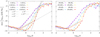 |
Fig. 1 Maximum relative variation in the Hamiltonian in Eq. (29) as a function of the time step used. We integrate a slightly perturbed isochrone potential where ε = 10−4. The integration is conducted over two radial periods (Δt = 2τ ≈ 239) of an orbit with unperturbed isochrone semi-major axis α ≈ 7.12 and eccentricity ε ≈ 4.21 × 10⁻¹. Black lines show several power laws for comparison. |
4 The isochrone splitting scheme
Now that all solutions of the isochrone dynamics are available, we can use them to build a symplectic splitting scheme, as described in Sect. 2. For sub-steps with Hamiltonian 𝒜 (i.e. an unperturbed isochrone motion), we used the formulas described in Sect. 3 to propagate any position and velocity (r, ![Mathematical equation: $\[\dot{\mathbf{r}}\]$](/articles/aa/full_html/2025/05/aa53886-25/aa53886-25-eq47.png) ) to their new value. We followed the standard methodology used for Kepler solvers (see e.g. Rein & Tamayo 2015). Yet, we did not find isochrone analogous versions of the Gauss functions f and g (Danby 1988), which means that our algorithm needs to compute the true anomaly φ explicitly. While doing so, we had to take special care that the value returned by the two arc-tangents (see the formulas in Sect. 3) lie in the correct quadrant of the trigonometric circle. The outline of an algorithm to compute the isochrone sub-steps is given in Appendix B.
) to their new value. We followed the standard methodology used for Kepler solvers (see e.g. Rein & Tamayo 2015). Yet, we did not find isochrone analogous versions of the Gauss functions f and g (Danby 1988), which means that our algorithm needs to compute the true anomaly φ explicitly. While doing so, we had to take special care that the value returned by the two arc-tangents (see the formulas in Sect. 3) lie in the correct quadrant of the trigonometric circle. The outline of an algorithm to compute the isochrone sub-steps is given in Appendix B.
To validate our analytical computations and numerical implementations, we first applied the isochrone splitting scheme to a slightly perturbed isochrone dynamics. We chose a dimensionless Hamiltonian function of the form
![Mathematical equation: $\[\mathcal{H}(\mathbf{r}, \dot{\mathbf{r}})=\frac{1}{2}\|\dot{\mathbf{r}}\|^2-\frac{\eta}{\kappa+\sqrt{\|\mathbf{r}\|^2+\kappa^2}}-\varepsilon \frac{\eta}{\|\mathbf{r}\|},\]$](/articles/aa/full_html/2025/05/aa53886-25/aa53886-25-eq48.png) (29)
(29)
where η = 1, κ = 1 and ε is a small quantity. To apply the isochrone splitting scheme, we split the Hamiltonian function as in Eqs. (10) and (11), in which ![Mathematical equation: $\[\Psi(r)=-\eta /\left(\kappa+\sqrt{r^{2}+\kappa^{2}}\right)-\varepsilon \eta / r\]$](/articles/aa/full_html/2025/05/aa53886-25/aa53886-25-eq49.png) and
and ![Mathematical equation: $\[\Phi(r)=-\mu /\left(b+\sqrt{r^{2}+b^{2}}\right)\]$](/articles/aa/full_html/2025/05/aa53886-25/aa53886-25-eq50.png) , where we chose μ = η and b = κ.
, where we chose μ = η and b = κ.
Figure 1 illustrates the results obtained for the 𝒮𝒜ℬ𝒜n, 𝒮ℬ𝒜ℬn, 𝒮𝒜ℬ𝒜𝒞n, and 𝒮ℬ𝒜ℬ𝒞n families of integrators, where n = 2 to 5. We note ℋ0 the Hamiltonian at the initial time and Δℋ its instantaneous variation relative to ℋ0 at time t. As introduced in Sect. 2, the integrators of Laskar & Robutel (2001) have errors of order 𝒪(εδt2n) + 𝒪(ε2δt2) for 𝒮𝒜ℬ𝒜n and 𝒮ℬ𝒜ℬn, and 𝒪(εδt2n) + 𝒪(ε2δt4) for 𝒮𝒜ℬ𝒜𝒞n and 𝒮ℬ𝒜ℬ𝒞n, where δt is the integration step. As expected, Fig. 1 shows that depending on the value of δt, either the first or the second error term dominates (see the curve slopes). This validates our implementation of the isochrone splitting scheme. As shown in Fig. 2, the use of a symplectic integrator (e.g. 𝒮𝒜ℬ𝒜2) with the isochrone splitting produces bounded energy variations, and no irreversible drift of energy over long timescales. In contrast, the RK4 non-symplectic integrator produces an energy drift that is visible within the first radial period.
To apply our splitting scheme to a generic potential Ψ(r), which may have an expression that greatly differs from the isochrone potential, we must find a generic way of choosing the parameters μ and b of the isochrone potential Φ(r) used for the splitting. To maximise the efficiency of our symplectic splitting scheme (see Sect. 2), we need to minimise the size of the perturbation εℬ as much as possible all along the trajectory. A possible choice is to set
![Mathematical equation: $\[\left\{\begin{array} { r } { ( \varepsilon \mathcal { B } ) _ { r = q } = 0 } \\{ ( \mathrm { d } _ { r } \varepsilon \mathcal { B } ) _ { r = q } = 0 }\end{array} \Longleftrightarrow \left\{\begin{array}{l}b=\left(\frac{r\left(1+r \frac{\mathrm{~d}_{r} \Psi}{\Psi}\right)}{\left.\sqrt{1-\left(1+r \frac{\mathrm{~d}_{r} \Psi}{\Psi}\right.}\right)^2}\right)_{r=q}\\\mu=-\left(\left(\sqrt{r^2+b^2}+b\right) \Psi\right)_{r=q}\end{array},\right.\right.\]$](/articles/aa/full_html/2025/05/aa53886-25/aa53886-25-eq51.png) (30)
(30)
where q is a given distance (e.g. the initial radial distance of the particle). This choice for the parameters μ and b implies that if εℬ solely depends on the radial distance r, the integration is exact whenever the star is located at a distance r = q. This parameter choice is studied in Sect. 5 for a Plummer potential. Equation (30) shows that this way of choosing the parameters μ and b for the isochrone splitting function Φ(r) cannot be applied to any potential Ψ(r); the following property must be satisfied:
![Mathematical equation: $\[-1 \leq\left(r \frac{\mathrm{~d}_r \Psi}{\Psi}\right)_{r=q}<0.\]$](/articles/aa/full_html/2025/05/aa53886-25/aa53886-25-eq52.png) (31)
(31)
If this condition is not verified, then the parameters μ and b must be chosen in a different way (see Sect. 7 for more details).
We note that, if we set b = 0, we retrieve the Kepler splitting scheme widely used in celestial mechanics; in that case, μ is generally chosen as the gravitational parameter of the central body (see e.g. Farrés et al. 2013; Hernandez & Dehnen 2017; Rein et al. 2019). Here, the addition of a second parameter – the length scale, b – gives us more freedom to adjust the integration scheme and adapt it to the particular problem under study.
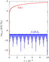 |
Fig. 2 Relative error in total energy as a function of time for the same orbit as in Fig. 1. The behaviour of two fourth-order integrators is shown: the Runge-Kutta method and the 𝒮𝒜ℬ𝒜2 method using the isochrone splitting (see the labels). A constant time step δt = 2.5 is used for both integrators. |
5 Application: Motion of a star in a Plummer potential
As a first experimentation of our new splitting scheme, we chose to solve for the motion of a star in a Plummer potential (Plummer 1911). The Plummer potential is the most simple galactic potential for which no closed-form analytic solution exists. The Plummer potential is an essential component of most galactic potentials (see e.g. Paczynski 1990; Allen & Santillan 1991; Pouliasis et al. 2017). It is therefore an unavoidable testbed for integrating the motion of stars in galaxies. This potential is expressed as
![Mathematical equation: $\[\Psi(\mathbf{r})=-\frac{\eta}{\sqrt{\|\mathbf{r}\|^2+\kappa^2}},\]$](/articles/aa/full_html/2025/05/aa53886-25/aa53886-25-eq53.png) (32)
(32)
where (η, κ) ∈ (ℝ+)2. Even though there is no closed-form solution for the motion of the star in this potential, we know that the motion is planar. Besides, the radial distance of the star either oscillates between the periapsis distance, rp, and the apoapsis distance, ra (bounded orbit), or it goes to infinity before and after reaching the star’s periapsis, rp (unbound orbit).
To apply our new splitting scheme and integrate the motion of the star, we divided the Hamiltonian function of the star as in Eq. (9) such that the perturbation is
![Mathematical equation: $\[\varepsilon \mathcal{B}(\mathbf{r})=\frac{\mu}{b+\sqrt{\|\mathbf{r}\|^2+b^2}}-\frac{\eta}{\sqrt{\|\mathbf{r}\|^2+\kappa^2}}.\]$](/articles/aa/full_html/2025/05/aa53886-25/aa53886-25-eq54.png) (33)
(33)
If εℬ is zero, then the star follows an isochrone orbit, and the solutions to the equations of motion are exact (see Sect. 4). Following Eq. (30), the isochrone mass parameter μ and scale radius b used for the splitting can be chosen as follows:
![Mathematical equation: $\[\left\{\begin{array}{l}b=\frac{\kappa}{\sqrt{2+(q / \kappa)^2}} \\\mu=\eta \sqrt{\frac{2+(q / \kappa)^2}{1+(q / \kappa)^2}},\end{array}\right.\]$](/articles/aa/full_html/2025/05/aa53886-25/aa53886-25-eq55.png) (34)
(34)
where q is an arbitrary value of r taken along the motion of the star7.
The optimal choice of the distance q chosen to compute μ and b in Eq. (34) is not trivial. With no lack of generality, we used normalised distances ![Mathematical equation: $\[\tilde{r}=r / \kappa\]$](/articles/aa/full_html/2025/05/aa53886-25/aa53886-25-eq56.png) and
and ![Mathematical equation: $\[\tilde{q}=q / \kappa\]$](/articles/aa/full_html/2025/05/aa53886-25/aa53886-25-eq57.png) and the normalised time
and the normalised time ![Mathematical equation: $\[\mathrm{d} \tilde{t}=(\eta / \kappa) \mathrm{d} t\]$](/articles/aa/full_html/2025/05/aa53886-25/aa53886-25-eq58.png) , which is equivalent to multiplying the total Hamiltonian function by the constant factor κ/η. In what follows, we drop the tilde symbol ‘~’ for readability. In this system of units, Eq. (33) can be expressed as
, which is equivalent to multiplying the total Hamiltonian function by the constant factor κ/η. In what follows, we drop the tilde symbol ‘~’ for readability. In this system of units, Eq. (33) can be expressed as
![Mathematical equation: $\[\varepsilon \mathcal{B}_q(r)=\frac{q^2+2}{\sqrt{q^2+1}\left(1+\sqrt{1+r^2\left(q^2+2\right)}\right)}-\frac{1}{\sqrt{1+r^2}}.\]$](/articles/aa/full_html/2025/05/aa53886-25/aa53886-25-eq59.png) (35)
(35)
We can prove that the function εℬq(r) is positive for any value of the variable r and parameter q (see Appendix C.1). To simplify the notations, we use below the index ‘p’ when q = rp and the index ‘a’ when q = ra.
Figure 3 shows the behaviour of εℬq(r) as a function of the parametrisation point q and the star’s radial location r. As the star moves between a periapsis and apoapsis, r varies between rp and ra, describing a horizontal segment in Fig. 3. Each parametrisation point q defines a given horizontal segment, and the collection of these segments form a square (see the example in red). For a given parameter q, we define the ‘perturbation index’ Pq as the maximum value of εℬq(r) for r ∈ [rp, ra]:
![Mathematical equation: $\[P_q=\max \left[\varepsilon \mathcal{B}_q(r)\right], \quad r \in\left[r_{\mathrm{p}}, r_{\mathrm{a}}\right].\]$](/articles/aa/full_html/2025/05/aa53886-25/aa53886-25-eq60.png) (36)
(36)
There exists a unique point rc > 0 such that ∂rεℬq(rc) = 0 and ![Mathematical equation: $\[\partial_{r r}^{2} \varepsilon \mathcal{B}_{q}\left(r_{\mathrm{c}}\right)<0\]$](/articles/aa/full_html/2025/05/aa53886-25/aa53886-25-eq61.png) , which corresponds to a local maximum. It can be shown than rc > q (see Appendix C.2). If we restrict r to lie in [rp, ra], then the maximum of εℬq(r) can be reached at rp, ra, or rc, that is,
, which corresponds to a local maximum. It can be shown than rc > q (see Appendix C.2). If we restrict r to lie in [rp, ra], then the maximum of εℬq(r) can be reached at rp, ra, or rc, that is,
![Mathematical equation: $\[P_q=\left\{\begin{array}{l}\max \left\{\varepsilon \mathcal{B}_q\left(r_{\mathrm{p}}\right), \varepsilon \mathcal{B}_q\left(r_{\mathrm{c}}\right)\right\} \text { when } r_{\mathrm{c}}<r_{\mathrm{a}}, \\\max \left\{\varepsilon \mathcal{B}_q\left(r_{\mathrm{p}}\right), \varepsilon \mathcal{B}_q\left(r_{\mathrm{a}}\right)\right\} \text { otherwise }.\end{array}\right.\]$](/articles/aa/full_html/2025/05/aa53886-25/aa53886-25-eq62.png) (37)
(37)
In particular, for q = ra, we always have Pa = εℬa(rp). The best parametrisation point q = q⋆ is that for which Pq is minimum; this minimum value, P⋆, is
![Mathematical equation: $\[P_{\star}=\min \left[P_q\right], \quad q \in\left[r_{\mathrm{p}}, r_{\mathrm{a}}\right].\]$](/articles/aa/full_html/2025/05/aa53886-25/aa53886-25-eq63.png) (38)
(38)
By definition, εℬp(rp) = 0, and εℬq(rp) is an increasing function of q. In contrast, εℬq(rc) and εℬq(ra) are decreasing function of q, and by definition εℬa(ra) = 0 (see Appendix C.1). Hence, the best parametrisation point q⋆ is
![Mathematical equation: $\[q_{\star}=\left\{q \text { such that } \varepsilon \mathcal{B}_q\left(r_{\mathrm{p}}\right)=\varepsilon \mathcal{B}_q\left(\min \left(r_{\mathrm{c}}, r_{\mathrm{a}}\right)\right)\right\}.\]$](/articles/aa/full_html/2025/05/aa53886-25/aa53886-25-eq64.png) (39)
(39)
We can compute it at an arbitrary precision using bisection.
Figure 4 shows the positions of the optimal parametrisation point q⋆ for orbits with periapsis and apoapsis distances ranging from 10−3 to 103 (in our system of units such that the Plummer scale radius is κ = 1). Three distinct regions can be identified: I. for rp > κ, we have q⋆ ≈ rp; II. for ra < κ, we have q⋆ ≈ ra; III. for rp < κ and ra > κ, we have q⋆ ≈ κ.
The performances of our splitting scheme can be evaluated by the size of the perturbation part εℬ (see Sect. 2). Here, the total Hamiltonian function is ![Mathematical equation: $\[\mathcal{H}=\|\dot{\mathbf{r}}\|^{2} / 2+\Psi(\mathbf{r})\]$](/articles/aa/full_html/2025/05/aa53886-25/aa53886-25-eq65.png) , where Ψ(r) is the Plummer potential. If we consider a bound orbit with pericentre rp and apocentre ra, then the constant value of ℋ is automatically set to ℋ = k, where
, where Ψ(r) is the Plummer potential. If we consider a bound orbit with pericentre rp and apocentre ra, then the constant value of ℋ is automatically set to ℋ = k, where
![Mathematical equation: $\[k=\frac{r_{\mathrm{p}}^2 \sqrt{1+r_{\mathrm{a}}^2}-r_{\mathrm{a}}^2 \sqrt{1+r_{\mathrm{p}}^2}}{\left(r_{\mathrm{a}}^2-r_{\mathrm{p}}^2\right) \sqrt{\left(1+r_{\mathrm{p}}^2\right)\left(1+r_{\mathrm{a}}^2\right)}} \in[-1,0).\]$](/articles/aa/full_html/2025/05/aa53886-25/aa53886-25-eq66.png) (40)
(40)
For given values of rp and ra, and a given parametrisation radius q ∈ [rp, ra], we define two quantities that characterise the performances of our splitting scheme: the size of the perturbation,
![Mathematical equation: $\[E_q=-\frac{P_q}{k}>0,\]$](/articles/aa/full_html/2025/05/aa53886-25/aa53886-25-eq67.png) (41)
(41)
and the relative magnitude of the perturbation,
![Mathematical equation: $\[\varepsilon_q=\frac{P_q}{\left|k-P_q\right|}>0.\]$](/articles/aa/full_html/2025/05/aa53886-25/aa53886-25-eq68.png) (42)
(42)
Namely, we have Eq ≈ |εℬ/ℋ|, and εq ≈ |εℬ/𝒜|. If Eq is small, then Eq ≈ εq, and both Eqs. (41) and (42) quantify the relative magnitude of the perturbation. Instead, when Eq is large, then εq ≈ 1 (i.e. there is no hierarchy between the ‘perturbation’ εℬ and the ‘unperturbed part’ 𝒜 in the Hamiltonian function). In that case Eq quantifies the magnitude of quantities that our splitting scheme artificially inserts in the Hamiltonian function, with no benefit on its performances.
The Ep, Ea, E⋆, and εp, εa, ε⋆ are the coefficients obtained when using a parametrisation radius q equal to rp, ra, or q⋆, respectively. Figure 5 shows the value of E⋆ and ε⋆ as a function of ra and rp. As expected, ε⋆ is very small when rp ≫ κ (Keplerian regime) and when ra ≪ κ (harmonic regime). We also obtain good performances when ra ≈ κ and/or rp ≈ κ, with values of ε⋆ of the order of 10−1 or 10−2. Yet, we expect no advantage of using our splitting scheme for highly eccentric orbits crossing the Plummer radius κ (i.e. for ra ≫ κ and rp < κ; see the red region in Fig. 5a), for which E⋆ > 10, and therefore ε⋆ ≈ 1.
This analysis shows that the best way to set up our splitting scheme depends on the properties of the trajectory followed by the star. However, in general we cannot know a priori what the star’s trajectory will be – we only know its initial conditions. Therefore, we must determine whether choosing the best parametrisation point q⋆ is critical to get the best performances of the integrator, or whether any other point along the star’s orbit (e.g. q = rp or ra, or the initial radial location) could give approximately similar performances.
Figure 6 shows how the perturbation sizes Ep and Ea behave relative to E⋆ as a function of ra and rp. Figure 6a shows that E⋆ and Ep only differ by a factor close to unity. Namely, Ep/E⋆ ≈ 2.5 in region I, Ep/E⋆ ≈ 3.5 in region II, and Ep/E⋆ ≈ 2 in region III. Moreover, we note that the largest ratio occurs in region II, where E⋆ is the smallest (see Fig. 5b). We conclude that using the parametrisation point q = rp instead of q = q⋆ would not damage too much the performances of our splitting scheme. In contrast, Fig. 6b shows that Ea is orders of magnitudes larger that E⋆ almost everywhere, except in region II and near the diagonal (for which ra ≈ rp anyway).
We conclude that choosing an adequate parametrisation point q ∈ [rp, ra] is indeed critical. Yet, choosing simply q = rp always give relevant results; it is therefore an easy choice to optimise the performance of the symplectic integrator developed in Sect. 4. We note that it remains true for unbound orbits.
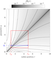 |
Fig. 3 Value of the Hamiltonian εℬq(r) in Eq. (35) as a function of the parametrisation point, q, and the star’s instantaneous position, r. The value of εℬq(r) is shown by the colour shades and black level curves. By definition of q, the value of εℬq(r) is zero along the diagonal (i.e. for r = q). An example of the periapsis, rp, apoapsis, ra, and best parametrisation point, q⋆, are shown in red and blue. In this system of units, the Plummer characteristic radius, κ, lies at r = 1. |
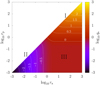 |
Fig. 4 Optimal parametrisation point, q⋆, as a function of the periapsis and apoapsis of the orbit. Some level curves appear in white. Regions I, II, and III are described in the text. |
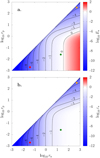 |
Fig. 5 Size, E⋆, of the perturbation (panel a) and relative magnitude, ε⋆, of the perturbation (panel b) computed for the optimal parametrisation point, q⋆. Some level curves appear in black. The three coloured points were used for the numerical experiments described in Sect. 6 (see Figs. 7 and 8). |
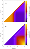 |
Fig. 6 Size, E, of the perturbation computed for q = rp (panel a) and q = ra (panel b) compared to the best parametrisation point, q⋆. The colour scale in panel a is linear; the colour scale in panel b is logarithmic. The level curve Ea/E⋆ = 10 is shown in white. The three coloured points were used for the numerical experiments described in Sect. 6 (see Figs. 7 and 8). |
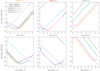 |
Fig. 7 Maximum relative variation in the Hamiltonian as a function of the integration time step over the radial period (top row) and as a function of the CPU integration time (bottom row). Each column corresponds to a different orbit (orange, red, and green points in Figs. 5 and 6), integrated over two radial periods with 𝒮𝒜ℬ𝒜1. The blue curve and the black curve show the results obtained when using kinetic splitting and Kepler splitting. The orange, green, and pink curves correspond to the isochrone splitting with parametrisation points q = rp, q = ra, and q = r⋆, respectively. |
6 Performance for stellar dynamics
In this section, we illustrate the properties obtained in Sect. 5 using numerical integrations. In galactic dynamics, the Plummer potential is often used to describe stellar clusters, in particular globular clusters. To illustrate the performances of our splitting scheme, we apply the symplectic integrator presented in Sect. 4 to a star orbiting in NGC 4372, assuming a Plummer distribution for the cluster. The total mass of NGC 4372 is M = 1.9 × 10⁵ ℳ⊙, and its half-mass radius is r1/2 = 8.34 pc, according to Baumgardt & Hilker (2018)8. The Plummer mass parameter, η, is related to the cluster’s mass by η = GM, where Gℳ⊙ = 4.49850 × 10⁻³ pc3 Myr−2 is the Solar gravitational parameter (Prša et al. 2016). The Plummer scale radius parameter, κ, is related to the half-mass radius by r1/2 ≃ 1.305κ (Heggie & Hut 2003). We do not mean here to reproduce the actual orbital evolution of stars within the NGC 4372 globular cluster, but only to illustrate our results using physically motivated parameter values for η and κ.
We considered three different orbits. These points are taken: in Region I (rp ≫ κ) and close to a circular orbit; in Region II (ra < κ); and in Region III (rp < κ and ra > κ). We call them respectively Orbit #1, Orbit #2, and Orbit #3. Their radial periods are respectively T ≈ 30 Gyr, 1.73 Myr, and 112 Myr. These trajectories are designed to test our integration scheme in a large variety of regimes, even extreme regimes (e.g. Orbit #1 may not be physically realistic).
Figure 7 shows the performances of the isochrone splitting scheme, as compared to the kinetic and Kepler splitting schemes. Integrations are performed with the widely used second-order symplectic integrator given in Eq. (7). This integrator is called 𝒮𝒜ℬ𝒜1 by Laskar & Robutel (2001) and it has errors of order 𝒪(εδt2). Kinetic splitting corresponds to Φ = 0 in Eqs. (10) and (11); when used with 𝒮𝒜ℬ𝒜1, it corresponds to the standard Leapfrog integrator (e.g. implemented in the Python package galpy). Kepler splitting uses Φ = μ/r, where we chose μ = GM. Kepler splitting involves a state-of-the-art two-body propagator, with in particular the Gauss functions f and g (see e.g. Danby 1988).
For Orbits #1 and #2, the choice of parametrisation point q for the isochrone potential does not affect much the integrator’s performance, as expected. The classic Leapfrog is outperformed by several orders of magnitude. Depending on the level of energy conservation requested, time step 100 to 1000 times larger can be used, with a noticeable benefit on the computation time (say, a factor of 10 to 100; see the bottom panels). Indeed, for these two orbits, the magnitude ε of the perturbation when using the isochrone splitting scheme is very small (see Sect. 5), which allows us to take full advantage of the hierarchical symplectic integrator.
For Orbit #3, the choice of parametrisation point q is important: if we choose q = ra, then the isochrone splitting scheme performs poorly – it is even less efficient than kinetic splitting. If we choose q = rp or q = r⋆ instead, we obtain a slightly better conservation of energy than kinetic splitting (top right panel), but an equivalent cost in terms of CPU time (bottom right panel). Indeed, for Orbit #3, the perturbation magnitude ε is close to unity (see the green point in Figs. 5 and 6). In such a case, there is no advantage in using a symplectic splitting scheme based on a particular hierarchy between the two terms of the Hamiltonian function.
Surprisingly, we note that for Orbit #3 the isochrone splitting scheme for q = rp performs slightly better than for q = q⋆; this is likely due to particular terms in the remainders of the integrator (see e.g. Laskar & Robutel 2001), which lose their well-behaved hierarchy when ε ≈ 1. This property confirms our conclusion from Sect. 5 that setting q = rp is an simple choice that optimises the isochrone splitting scheme.
As expected, Kepler splitting performs similarly as the isochrone splitting for Orbit #1 (see the black curve in Fig. 7), because this orbit is far from the centre of the cluster. However, Kepler splitting shows very poor performances for Orbits #2 and #3, which are strongly non-Keplerian. This illustrates that the isochrone splitting is a generalisation of Kepler splitting: it works equally well for perturbed Keplerian orbits but it has a wider range of applications.
The improved hierarchy (i.e. small value of ε) when using the isochrone splitting implies that if a better conservation of energy is needed, more advanced integrators will converge faster to a high precision. This property is illustrated in Fig. 8, showing the results obtained with the integrator 𝒮𝒜ℬ𝒜3, which has errors of the form 𝒪(εδt6) + 𝒪(ε2δt2). For large time steps, the slope 6 is clearly visible (as compared to the slope 2 in Fig. 7). In contrast, the slope remains unchanged for kinetic splitting, because the second error terms in 𝒪(ε2δt2) dominates. However, as discussed in Sect. 1 high precision integrations are generally not needed in the context of galactic dynamics.
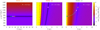 |
Fig. 9 Maximum relative variation in the Hamiltonian as a function of the parameters μ and b of the isochrone potential used for the splitting. Each column corresponds to a different orbit (orange, red, and green points in Figs. 5 and 6), integrated with 𝒮𝒜ℬ𝒜1 over two radial periods for a given integration time step, δt. The orange, green, and pink points correspond to the isochrone splitting with parametrisation points q = rp, q = ra, and q = r⋆, respectively (the points overlap for Orbit #2), while the cyan curve shows all possible parametrisation points, q, between the periapsis distance and apoapsis distance, following Eq. (34). |
7 Discussion
Similarly to other splitting schemes (see e.g. Hernandez & Dehnen 2017), the choice of the isochrone parameters μ and b made in Eq. (30) is not unique. We used Eq. (30) as an attempt to minimise the perturbation Hamiltonian εℬ in a simple way, but other choices for μ and b could possibly yield equal performances, or even better performances than what we obtained in Sect. 5.
Figure 9 illustrates the integrator’s performance as a function of the splitting parameters, which do not specifically follow Eq. (30), for the three orbits presented in Sect. 6. For all three orbits, we observe that there is a region where the performance of the integrator is much better. The choice made in Sect. 4 falls within this region for a well-chosen parametrisation point q. As we mentioned in Sect. 6, the parametrisation at the periapsis distance slightly outperforms the parametrisation at the optimal point defined in Eq. (39) for the Orbit #3. Indeed, the characteristic size of the perturbation for Orbit #3 is ε ≈ 1 (see Fig. 5), so we expect a poor convergence of the remainders as expressed in powers of ε. As a result the exact minimum of ε does not necessarily gives exactly the best performances of the integrator, depending on the splitting scheme used, but it comes close.
8 Summary and conclusions
In many studies of stellar and galactic dynamics, it is necessary to numerically integrate a large number of test particles (typically stars) in some smoothed gravitational potential. Symplectic integrators are widely used in this context because of their exquisite stability properties. To date, the vast majority of studies have used the kinetic symplectic splitting scheme, for which the integrator alternates between a linear drift and a velocity kick (see e.g. Martínez-Barbosa et al. 2015; Pouliasis et al. 2017; Ferrone et al. 2023). However, much more efficient symplectic integrators have been developed for cases where the Hamiltonian has a particular hierarchical structure (e.g. a dominant part plus a perturbation; see Wisdom & Holman 1991; McLachlan 1995; Laskar & Robutel 2001). We investigated whether such integrators can be advantageous for stellar dynamics with an appropriate choice of splitting.
In this regard, Hénon’s isochrone potential seems very promising because it shares many properties with complex galactic potentials (e.g. it is harmonic at short distances and Keplerian at large distances), and the isochrone dynamics is fully integrable analytically. Therefore, we used Hénon’s isochrone potential as a basis for a new splitting scheme, for which the integrator alternates between an isochrone drift (Hamiltonian 𝒜) and a velocity kick (Hamiltonian εℬ). To this end, we have expressed all solutions of the isochrone dynamics – including unbound trajectories – in an explicit form, by introducing an ‘eccentric anomaly’ similar to the Keplerian one. The problem then becomes one of selecting the mass parameter, μ, and the characteristic distance, b, of the isochrone potential used in the integration scheme such that the characteristic magnitude, ε, of the perturbations is minimised.
As a first application of this splitting scheme, we integrated the motion of stars in a Plummer potential – which is an essential component of most galactic potentials. In this case, we have shown that a judicious choice for μ and b is to set εℬ and its first derivative to zero at the star’s periapsis. This way, ε takes very small values for a large fraction of trajectories: typically 10−6 for stars near the centre of the mass distribution (harmonic regime) and 10−3 for stars in the periphery of the distribution (Keplerian regime). Poorer performances are obtained for stars on very elongated orbits that cross the Plummer characteristic radius, for which ε ~ 1.
Numerical experiments show that, depending on the dynamical regime of the star considered, this new splitting scheme can outperform the standard Leapfrog integrator by several orders of magnitude. As a result, computations are faster by a factor of 10 to 100 for the same energy conservation. In the worst cases – very elongated orbits that cross both inner and outer regions of the Plummer distribution – performances are equivalent to those obtained with previous integration methods.
The isochrone splitting scheme introduced here remains to be explored for more general potentials among those used in galactic dynamics. In these future applications, the parameters μ and b will need to be chosen in an adequate way, depending on the potentials included. The results obtained here give us confidence that good performances will be obtained in future applications. We expect clear improvements compared to previous methods at least for some classes of stellar trajectories.
According to the specific implementation methodology, the method presented here could be improved in many ways in the future. For instance, analogous versions of the Gauss functions f and g could be derived for the isochrone dynamics, and round-off errors and computation times could be optimised more than in our proof-of-concept implementation presented here. We leave such refinements for future studies.
Acknowledgements
We thank Alain Vienne for useful discussions about numerical cancellation errors. We also thank the anonymous reviewer for his/her very thorough review that greatly improved the clarity of our manuscript. This work was supported by the Programme de Planétologie (PNP) of CNRS/INSU, co-funded by CNES.
References
- Allen, C., & Santillan, A. 1991, Rev. Mexicana Astron. Astrofis., 22, 255 [Google Scholar]
- Baba, J., Tsujimoto, T., & Saitoh, T. R. 2024, ApJ, 976, L29 [Google Scholar]
- Baumgardt, H., & Hilker, M. 2018, MNRAS, 478, 1520 [Google Scholar]
- Bertrand, J. L. F. 1873, Comp. Rend. Hebdomadaires Séances Acad. Sci., 77, 849 [Google Scholar]
- Binney, J. 2016, in Une vie dédiée aux systèmes dynamiques : Hommage à Michel Hénon, eds. J.-M. Alimi, R. Mohayaee, & J. Perez (Hermann), 99 [CrossRef] [Google Scholar]
- Binney, J., & Tremaine, S. 2008, Galactic Dynamics, 2nd edn. (Princeton University Press) [Google Scholar]
- Blanes, S., Casas, F., Farrés, A., et al. 2013, Appl. Numer. Math., 68, 58 [Google Scholar]
- Boulila, S., Laskar, J., Haq, B. U., Galbrun, B., & Hara, N. 2018, Global Planet. Change, 165, 128 [CrossRef] [Google Scholar]
- Bovy, J. 2015, ApJS, 216, 29 [NASA ADS] [CrossRef] [Google Scholar]
- Caritá, L. A., Rodrigues, I., Puerari, I., & Schiavo, L. E. C. A. 2018, New A, 60, 48 [Google Scholar]
- Chambers, J. E. 1999, MNRAS, 304, 793 [Google Scholar]
- Danby, J. M. A. 1988, Fundamentals of Celestial Mechanics (Atlantic Books) [Google Scholar]
- Dinescu, D. I., Girard, T. M., & van Altena, W. F. 1999, AJ, 117, 1792 [Google Scholar]
- Farrés, A., Laskar, J., Blanes, S., et al. 2013, Celest. Mech. Dyn. Astron., 116, 141 [Google Scholar]
- Ferrone, S., Di Matteo, P., Mastrobuono-Battisti, A., et al. 2023, A&A, 673, A44 [NASA ADS] [CrossRef] [EDP Sciences] [Google Scholar]
- Forest, E., & Ruth, R. D. 1990, Physica D Nonlinear Phenomena, 43, 105 [Google Scholar]
- Gardner, E., Nurmi, P., Flynn, C., & Mikkola, S. 2011, MNRAS, 411, 947 [Google Scholar]
- Greiner, J. 1987, Celest. Mech., 40, 171 [Google Scholar]
- Hairer, E., Wanner, G., & Lubich, C. 2006, Geometric Numerical Integration (Berlin, Heidelberg: Springer) [Google Scholar]
- Heggie, D., & Hut, P. 2003, The Gravitational Million-Body Problem: A Multidisciplinary Approach to Star Cluster Dynamics (Cambridge University Press) [Google Scholar]
- Hénon, M. 1959a, Ann. Astrophys., 22, 491 [Google Scholar]
- Hénon, M. 1959b, Ann. Astrophys., 22, 126 [Google Scholar]
- Hernandez, D. M., & Dehnen, W. 2017, MNRAS, 468, 2614 [Google Scholar]
- Hernandez, D. M., & Dehnen, W. 2024, MNRAS, 530, 3870 [Google Scholar]
- Hernandez, D. M., Hadden, S., & Makino, J. 2020, MNRAS, 493, 1913 [NASA ADS] [CrossRef] [Google Scholar]
- Ibata, R. A., Malhan, K., & Martin, N. F. 2019, ApJ, 872, 152 [Google Scholar]
- Kaib, N. A., Roškar, R., & Quinn, T. 2011, Icarus, 215, 491 [Google Scholar]
- Khalil, Y. R., Famaey, B., Monari, G., et al. 2024, A Non-axisymmetric Potential for the Milky Way Disk [arXiv:2411.12800] [Google Scholar]
- Khoperskov, S., Di Matteo, P., Haywood, M., Gómez, A., & Snaith, O. N. 2020, A&A, 638, A144 [NASA ADS] [CrossRef] [EDP Sciences] [Google Scholar]
- Kinoshita, H., Yoshida, H., & Nakai, H. 1990, Celest. Mech. Dyn. Astron., 50, 59 [Google Scholar]
- Laskar, J., & Robutel, P. 2001, Celest. Mech. Dyn. Astron., 80, 39 [NASA ADS] [CrossRef] [Google Scholar]
- Martínez-Barbosa, C. A., Brown, A. G. A., & Portegies Zwart, S. 2015, MNRAS, 446, 823 [Google Scholar]
- Martínez-Barbosa, C. A., Jílková, L., Portegies Zwart, S., & Brown, A. G. A. 2017, MNRAS, 464, 2290 [Google Scholar]
- McLachlan, R. I. 1995, BIT Numer. Math., 35, 258 [Google Scholar]
- Miyamoto, M., & Nagai, R. 1975, Astron. Soc. Jpn., 27, 533 [Google Scholar]
- Paczynski, B. 1990, ApJ, 348, 485 [NASA ADS] [CrossRef] [Google Scholar]
- Pascale, R., Nipoti, C., & Ciotti, L. 2022, MNRAS, 509, 1465 [Google Scholar]
- Pérez-Villegas, A., Rossi, L., Ortolani, S., et al. 2018, PASA, 35, e021 [CrossRef] [Google Scholar]
- Pichardo, B., Martos, M., & Moreno, E. 2004, ApJ, 609, 144 [NASA ADS] [CrossRef] [Google Scholar]
- Plummer, H. C. 1911, MNRAS, 71, 460 [Google Scholar]
- Portegies Zwart, S., & Boekholt, T. 2014, ApJ, 785, L3 [NASA ADS] [CrossRef] [Google Scholar]
- Pouliasis, E., Di Matteo, P., & Haywood, M. 2017, A&A, 598, A66 [NASA ADS] [CrossRef] [EDP Sciences] [Google Scholar]
- Prša, A., Harmanec, P., Torres, G., et al. 2016, AJ, 152, 41 [Google Scholar]
- Ramond, P., & Perez, J. 2020, Celest. Mech. Dyn. Astron., 132, 22 [Google Scholar]
- Ramond, P., & Perez, J. 2021, J. Math. Phys., 62, 112704 [Google Scholar]
- Rein, H., & Tamayo, D. 2015, MNRAS, 452, 376 [Google Scholar]
- Rein, H., Tamayo, D., & Brown, G. 2019, MNRAS, 489, 4632 [NASA ADS] [CrossRef] [Google Scholar]
- Ruth, R. D. 1983, IEEE Trans. Nucl. Sci., 30, 2669 [Google Scholar]
- Saillenfest, M. 2020, Celest. Mech. Dyn. Astron., 132, 1 [Google Scholar]
- Sharina, M., Ryabova, M., Maricheva, M., & Gorban, A. 2018, Astron. Rep., 62, 733 [Google Scholar]
- Simon-Petit, A., Perez, J., & Duval, G. T. 2018, Commun. Math. Phys., 363, 605 [Google Scholar]
- Simon-Petit, A., Perez, J., & Plum, G. 2019, MNRAS, 484, 4963 [Google Scholar]
- Smirnova, L. V. 2015, Open Astron., 24, 209 [Google Scholar]
- Wisdom, J., & Holman, M. 1991, AJ, 102, 1528 [Google Scholar]
- Wisdom, J., & Hernandez, D. M. 2015, MNRAS, 453, 3015 [Google Scholar]
- Yoshida, H. 1990, Phys. Lett. A, 150, 262 [NASA ADS] [CrossRef] [Google Scholar]
- Yoshida, H. 1993, Celest. Mech. Dyn. Astron., 56, 27 [NASA ADS] [CrossRef] [Google Scholar]
- Zotos, E. E. 2014, Mech. Res. Commun., 62, 102 [Google Scholar]
Appendix A Bounded Hénon’s isochrone orbits
A.1 Deriving the time dependence
The change of variable
![Mathematical equation: $\[u=\sqrt{1+(r / b)^2}\]$](/articles/aa/full_html/2025/05/aa53886-25/aa53886-25-eq69.png)
in the energy equation in Eq. (13) allows us to obtain the following non-linear differential equation:
![Mathematical equation: $\[\left(\mathrm{d}_t u^2\right)^2=4\left(k_3\left(u^2-1\right)+k_2(u-1)-k_1\right),\]$](/articles/aa/full_html/2025/05/aa53886-25/aa53886-25-eq70.png) (A.1)
(A.1)
where k1 = (Λ/b2)2, k2 = 2μ/b3, and k3 = 2h/b2. The next change of variable,
![Mathematical equation: $\[s=\mathbf{r} \cdot \dot{\mathbf{r}}=\sqrt{k_3\left(u^2-1\right)+k_2(u-1)-k_1},\]$](/articles/aa/full_html/2025/05/aa53886-25/aa53886-25-eq71.png)
allows us to integrate the previous equation:
![Mathematical equation: $\[\Delta t=\frac{1}{k_3} \int \mathrm{~d} s-\frac{k_2}{2 k_3} \underbrace{\int \frac{\mathrm{~d} u}{\sqrt{k_3\left(u^2-1\right)+k_2(u-1)-k_1}}}_I,\]$](/articles/aa/full_html/2025/05/aa53886-25/aa53886-25-eq72.png) (A.2)
(A.2)
where the quantity I (see the bottom curly bracket in Eq. (A.2)) can be rewritten as
![Mathematical equation: $\[\begin{aligned}I \sqrt{k_3} & =\int \frac{\mathrm{d} v}{\sqrt{v^2-k_4}} \\& =\ln \left(\sqrt{v^2-k_4}+v\right) \\& =\operatorname{arctanh}\left(\frac{v}{\sqrt{v^2-k_4}}\right) \\& =\operatorname{arctanh}\left(\frac{\mathrm{d}_u s}{\sqrt{k_3}}\right).\end{aligned}\]$](/articles/aa/full_html/2025/05/aa53886-25/aa53886-25-eq73.png)
Here, we have defined v = u + k2/2k3 and ![Mathematical equation: $\[k_{4}= \left(4 k_{3}\left(k_{1}+k_{2}+k_{3}\right)+k_{2}^{2}\right) / 4 k_{3}^{2}\]$](/articles/aa/full_html/2025/05/aa53886-25/aa53886-25-eq74.png) . So, the time it takes for a particle to move between two positions is finally given by
. So, the time it takes for a particle to move between two positions is finally given by
![Mathematical equation: $\[\begin{aligned}\Delta t & =\frac{s}{k_3}-\frac{k_2}{2 k_3^{3 / 2}} \operatorname{arctanh}\left(\frac{\mathrm{~d}_u s}{\sqrt{k_3}}\right) \\& =\frac{\mathbf{r} \cdot \dot{\mathbf{r}}}{2 h}-\frac{\mu}{\sqrt{2 h^3}} \operatorname{arctanh}\left(\frac{1}{\sqrt{2 h}} \mathrm{~d}_{\sqrt{r^2+b^2}}(\mathbf{r} \cdot \dot{\mathbf{r}})\right).\end{aligned}\]$](/articles/aa/full_html/2025/05/aa53886-25/aa53886-25-eq75.png)
A.2 Orbit classification
Figure A.1 shows an example of a bounded particle’s Hénon isochrone trajectory. Bounded orbits form a series of loops, where each loop is shifted by
![Mathematical equation: $\[\Delta \varphi=\pi\left(1+\frac{\Lambda}{\sqrt{\Lambda^2+4 b \mu}}\right),\]$](/articles/aa/full_html/2025/05/aa53886-25/aa53886-25-eq76.png) (A.3)
(A.3)
after each radial period. The curvilinear length of each loop is given by
![Mathematical equation: $\[\Gamma=\alpha \int_0^{2 \pi}(1-\epsilon ~\cos~ E) \sqrt{\frac{\alpha(1+\epsilon \cos E)-b}{\alpha(1-\epsilon ~\cos~ E)+b}} \mathrm{~d} E.\]$](/articles/aa/full_html/2025/05/aa53886-25/aa53886-25-eq77.png) (A.4)
(A.4)
Depending on the possible combinations of values for the particle’s orbital parameters – semi-major axis, α, and eccentricity, ε – and the isochrone characteristic length parameter b9, the geometric shape of the orbit resulting from the succession of loops differs:
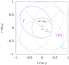 |
Fig. A.1 Example of a particle’s motion in its orbital plane (a special case of a closed orbit where Δφ = 3π/2) with the isochrone parameters μ = 1 and b = 2 × 10⁻¹. The green and blue circles, labelled Crp and Cra, respectively show the particle’s minimum and maximum radial positions. The dashed violet line, denoted by r(t), shows the particle’s orbit. The solid violet line shows the path of the particle during one radial period; its length is given by Γ (see Eq. (A.4)). The small arrow indicates the rotational sense of the loops. |
When b = 0, orbits are Keplerian ellipses.
When α = b, the eccentricity necessarily becomes zero (see Eq. (22)), implying that Γ = 0 : the particle remains unmoved at the origin.
When ε = 0 and 0 ≤ b < α, Eq. (A.4) reduces to the integral of the perimeter of a circle, and the trajectory depicts a circle with radius given in Eq. (21).
When ε = 1 – b/α, the angular momentum is zero. Equation (A.4) reduces to the integral of the length of a straight line, and the orbit is a line segment, as shown by Eqs. (21) and (23).
The other cases are rosette-shaped, characterised by two periods: a radial and an apsidal period.
All different classes of bounded orbits are summarised in Table 1. The orbit is closed if and only if the radial and apsidal periods are multiples of each other, in which case Δφ ∈ 2πℚ, which is a necessary and sufficient condition. Bertrand’s theorem indicates that, in the family of all isochrone potentials (see Simon-Petit et al. 2018), only the Keplerian and harmonic potentials have all their bound orbits closed (Bertrand 1873). Figure A.1 shows a case where a bound Hénon isochrone orbit is closed.
A.3 Polar angle
For a bound orbit, the polar angle φ as a function of the eccentric anomaly given in Eq. (23) can be rewritten as
![Mathematical equation: $\[\begin{aligned}\varphi(E)= & \frac{\Lambda}{\sqrt{\Lambda^2+4 b \mu}} \arctan \left(\sqrt{\frac{\mu \alpha}{\Lambda^2+4 b \mu}}\left(1+\frac{b}{\alpha}+\epsilon\right) \tan \left(\frac{E}{2}\right)\right) \\& +\arctan \left(\frac{\sqrt{\mu \alpha}\left(1-\frac{b}{\alpha}+\epsilon\right)}{\Lambda} \tan \left(\frac{E}{2}\right)\right) \\= & \frac{\Lambda}{\sqrt{\Lambda^2+4 b \mu}} \arctan \left(\frac{1+\frac{b}{\alpha}+\epsilon}{1+\epsilon-\frac{\sqrt{r^2+b^2}}{\alpha}} \frac{\mathbf{r} \cdot \dot{\mathbf{r}}}{\sqrt{\Lambda^2+4 b \mu}}\right) \\& +\arctan \left(\frac{1-\frac{b}{\alpha}+\epsilon}{1+\epsilon-\frac{\sqrt{r^2+b^2}}{\alpha}} \frac{\mathbf{r} \cdot \dot{\mathbf{r}}}{\Lambda}\right),\end{aligned}\]$](/articles/aa/full_html/2025/05/aa53886-25/aa53886-25-eq78.png)
where we have used
![Mathematical equation: $\[\left\{\begin{array}{l}\epsilon ~\cos~ E=1-\frac{\sqrt{r^2+b^2}}{\alpha} \\\epsilon ~\sin~ E=\frac{\mathbf{r} ~\cdot ~\dot{\mathbf{r}}}{\sqrt{\mu \alpha}}\end{array}.\right.\]$](/articles/aa/full_html/2025/05/aa53886-25/aa53886-25-eq79.png)
This form of the equation is more convenient when we take the limit as the energy h tends towards zero in Sect. 3.3. In this case, ![Mathematical equation: $\[\alpha \underset{h \rightarrow 0}\longrightarrow{ } \infty\]$](/articles/aa/full_html/2025/05/aa53886-25/aa53886-25-eq80.png) .
.
Appendix B Algorithm for the isochrone sub-steps
In this section we outline an algorithm to propagate a particle from the state vector (r0, ![Mathematical equation: $\[\dot{\mathbf{r}}\]$](/articles/aa/full_html/2025/05/aa53886-25/aa53886-25-eq81.png) 0) at time t0 to the state vector (r,
0) at time t0 to the state vector (r, ![Mathematical equation: $\[\dot{\mathbf{r}}\]$](/articles/aa/full_html/2025/05/aa53886-25/aa53886-25-eq82.png) ) at time t = t0 + δt following the isochrone dynamics with parameters μ and b. We start by computing the angular momentum Λ and energy h as
) at time t = t0 + δt following the isochrone dynamics with parameters μ and b. We start by computing the angular momentum Λ and energy h as
![Mathematical equation: $\[\begin{aligned}\mathbf{\Lambda} & =\mathbf{r}_0 \times \dot{\mathbf{r}}_0 \\z & =\frac{\left\|\dot{\mathbf{r}}_0\right\|}{\mu}-\frac{2}{b+\sqrt{r_0^2+b^2}}\end{aligned}.\]$](/articles/aa/full_html/2025/05/aa53886-25/aa53886-25-eq83.png) (B.1)
(B.1)
We note that z is equal to 2h/μ. According to the value of z, we select the type of trajectory followed by the particle (see Sect. 3). If z < 0, the trajectory is bound and z is equal to −1/α. We then compute k0 = ε cos E0 and l0 = ε sin E0 as
![Mathematical equation: $\[\begin{aligned}& k_0=1+z \sqrt{r_0^2+b^2}, \\& l_0=\mathbf{r}_0 \cdot \dot{\mathbf{r}}_0 \sqrt{-\frac{z}{\mu}},\end{aligned}\]$](/articles/aa/full_html/2025/05/aa53886-25/aa53886-25-eq84.png) (B.2)
(B.2)
and the variation of mean anomaly as ![Mathematical equation: $\[\delta M=\delta t \sqrt{-z^{3} \mu}\]$](/articles/aa/full_html/2025/05/aa53886-25/aa53886-25-eq85.png) . We can now solve the variational Kepler equation,
. We can now solve the variational Kepler equation,
![Mathematical equation: $\[\delta M-l_0=\delta E-k_0 ~\sin~ \delta E-l_0 ~\cos~ \delta E,\]$](/articles/aa/full_html/2025/05/aa53886-25/aa53886-25-eq86.png) (B.3)
(B.3)
for the variation δE in eccentric anomaly. This step is realised with a root-finding algorithm that converges to machine precision within a few iterations (typically two) for any value of k0, l0, and δM.
At that point, as we did not find an isochrone version of the Gauss functions f and g (see e.g. Danby 1988), a few operations still need to be performed. We first compute the unitary vector ![Mathematical equation: $\[\hat{\boldsymbol{\epsilon}}\]$](/articles/aa/full_html/2025/05/aa53886-25/aa53886-25-eq87.png) pointing towards the previous periapsis,
pointing towards the previous periapsis,
![Mathematical equation: $\[\hat{\boldsymbol{\epsilon}}=\left(\hat{\boldsymbol{\Lambda}} \times \hat{\mathbf{r}}_0\right) \times \hat{\boldsymbol{\Lambda}} ~\cos~ \varphi_0-\hat{\boldsymbol{\Lambda}} \times \hat{\mathbf{r}}_0 ~\sin~ \varphi_0,\]$](/articles/aa/full_html/2025/05/aa53886-25/aa53886-25-eq88.png) (B.4)
(B.4)
where ![Mathematical equation: $\[\hat{\boldsymbol{\Lambda}}=\boldsymbol{\Lambda} / \Lambda, \hat{\mathbf{r}}_{0}=\mathbf{r}_{0} / r_{0}\]$](/articles/aa/full_html/2025/05/aa53886-25/aa53886-25-eq89.png) , and the initial true anomaly φ0 is computed from E0 = atan2(l0, k0) using Eq. (23). The vector
, and the initial true anomaly φ0 is computed from E0 = atan2(l0, k0) using Eq. (23). The vector ![Mathematical equation: $\[\hat{\boldsymbol{\epsilon}}\]$](/articles/aa/full_html/2025/05/aa53886-25/aa53886-25-eq90.png) is needed to compute the rotation matrix ℛ that converts a vector expressed in the orbital reference frame (i.e. with first axis
is needed to compute the rotation matrix ℛ that converts a vector expressed in the orbital reference frame (i.e. with first axis ![Mathematical equation: $\[\hat{\boldsymbol{\epsilon}}\]$](/articles/aa/full_html/2025/05/aa53886-25/aa53886-25-eq91.png) and third axis
and third axis ![Mathematical equation: $\[\hat{\boldsymbol{\Lambda}}\]$](/articles/aa/full_html/2025/05/aa53886-25/aa53886-25-eq92.png) ) to the working reference frame. The three columns of matrix ℛ are respectively
) to the working reference frame. The three columns of matrix ℛ are respectively ![Mathematical equation: $\[\hat{\boldsymbol{\epsilon}}, \hat{\boldsymbol{\Lambda}} \times \hat{\boldsymbol{\epsilon}}\]$](/articles/aa/full_html/2025/05/aa53886-25/aa53886-25-eq93.png) , and
, and ![Mathematical equation: $\[\hat{\boldsymbol{\Lambda}}\]$](/articles/aa/full_html/2025/05/aa53886-25/aa53886-25-eq94.png) .
.
The new distance r of the particle is computed as
![Mathematical equation: $\[r^2=r_0^2+p\left(p-2 \sqrt{r_0^2+b^2}\right),\]$](/articles/aa/full_html/2025/05/aa53886-25/aa53886-25-eq95.png) (B.5)
(B.5)
where
![Mathematical equation: $\[p=\frac{1}{z}\left(2\left(1+z \sqrt{r_0^2+b^2}\right) ~\sin~ ^2 \frac{\delta E}{2}+l_0 ~\sin~ \delta E\right).\]$](/articles/aa/full_html/2025/05/aa53886-25/aa53886-25-eq96.png) (B.6)
(B.6)
Equation (B.5) is equivalent to Eq. (21) but it avoids dramatic cancellation errors occurring whenever r ≪ b. We also computed the quantity s = r · ![Mathematical equation: $\[\dot{\mathbf{r}}\]$](/articles/aa/full_html/2025/05/aa53886-25/aa53886-25-eq97.png) as
as
![Mathematical equation: $\[s=\sqrt{-\frac{\mu}{z}} \epsilon ~\sin~ E,\]$](/articles/aa/full_html/2025/05/aa53886-25/aa53886-25-eq98.png) (B.7)
(B.7)
where ![Mathematical equation: $\[\epsilon=\sqrt{k_{0}^{2}+l_{0}^{2}}\]$](/articles/aa/full_html/2025/05/aa53886-25/aa53886-25-eq99.png) and E = E0 + δE. Expressed in the orbital reference frame, the new position vector of the particle has components (r cos φ, r sin φ, 0), and the new velocity vector has components (s cos φ − Λ sin φ, Λ cos φ + s sin φ, 0/r, where the true anomaly φ is computed from E using Eq. (23). It now remains to multiply these two vectors by the matrix ℛ, which finally gives the position r and velocity
and E = E0 + δE. Expressed in the orbital reference frame, the new position vector of the particle has components (r cos φ, r sin φ, 0), and the new velocity vector has components (s cos φ − Λ sin φ, Λ cos φ + s sin φ, 0/r, where the true anomaly φ is computed from E using Eq. (23). It now remains to multiply these two vectors by the matrix ℛ, which finally gives the position r and velocity ![Mathematical equation: $\[\dot{\mathbf{r}}\]$](/articles/aa/full_html/2025/05/aa53886-25/aa53886-25-eq100.png) of the particle in the working reference frame.
of the particle in the working reference frame.
Unbound trajectories (i.e. when h ≥ 0) and special cases (e.g. when Λ = 0) are treated in a similar manner with the corresponding formulas.
Appendix C Properties of the function εℬq(r)
In this section we study the properties of the continuous and differentiable function εℬq(r), defined in Eq. (35) as
![Mathematical equation: $\[\varepsilon \mathcal{B}_q(r)=\frac{q^2+2}{\sqrt{q^2+1}\left(1+\sqrt{1+r^2\left(q^2+2\right)}\right)}-\frac{1}{\sqrt{1+r^2}},\]$](/articles/aa/full_html/2025/05/aa53886-25/aa53886-25-eq101.png) (C.1)
(C.1)
where r ≥ 0 is the particle’s radial position, and q ≥ 0 is the distance used as parameter.
C.1 Positive function
We have the following demonstrated propositions:
-
![Mathematical equation: $\[\left\{\begin{array}{rl}\varepsilon \mathcal{B}_q(r) & =0 \\\partial_q \varepsilon \mathcal{B}_q(r) & =0\end{array} \quad \Longleftrightarrow \quad r=q.\right.\]$](/articles/aa/full_html/2025/05/aa53886-25/aa53886-25-eq102.png)
As a function of q, the function εℬq(r) is monotonically decreasing for q ∈ (0, r), because ∂qεℬq(r) < 0.
As a function of q, the function εℬq(r) is monotonically increasing for q > r, because ∂qεℬq(r) ≥ 0.
-
![Mathematical equation: $\[\begin{aligned}& \varepsilon \mathcal{B}_0(r)=\frac{2}{1+\sqrt{1+2 r^2}}-\frac{1}{\sqrt{1+r^2}} \geq 0, \\& \lim _{q \rightarrow \infty} \varepsilon \mathcal{B}_q(r)=\frac{1}{r}-\frac{1}{\sqrt{1+r^2}}>0.\end{aligned}\]$](/articles/aa/full_html/2025/05/aa53886-25/aa53886-25-eq103.png)
From this set of propositions, we deduce that
![Mathematical equation: $\[\varepsilon \mathcal{B}_q(r) \geq 0 \forall(q, r) \in \mathbb{R}_{+}^2.\]$](/articles/aa/full_html/2025/05/aa53886-25/aa53886-25-eq104.png)
C.2 Extrema of εℬq(r)
The derivative of εℬq(r) with respect to r is a sum of two terms (see Eq. (35)). By factorising the equation and multiplying the numerator by its conjugate to elevate both terms to the square, we obtain
![Mathematical equation: $\[\partial_r \varepsilon \mathcal{B}_q=\frac{r\left(x-x_q\right) p_5(x)}{w},\]$](/articles/aa/full_html/2025/05/aa53886-25/aa53886-25-eq105.png) (C.2)
(C.2)
where w is a strictly positive quantity for any r, q ≥ 0, and p5(x) is a polynomial of order 5 in x that does not cancel in x = xq. In this expression, we have written ![Mathematical equation: $\[x=\sqrt{1+r^{2}\left(q^{2}+2\right)}\]$](/articles/aa/full_html/2025/05/aa53886-25/aa53886-25-eq106.png) and xq = 1 + q2. The expression of p5(x) is
and xq = 1 + q2. The expression of p5(x) is
![Mathematical equation: $\[\begin{aligned}p_5(x)= & -x^5+3 x_q x^4+3 x_q x^3+x_q\left(3 x_q+4\right) x^2 \\& +x_q\left(x_q+1\right) x+x_q^2\left(x_q+1\right).\end{aligned}\]$](/articles/aa/full_html/2025/05/aa53886-25/aa53886-25-eq107.png) (C.3)
(C.3)
The function ∂rεℬq in Eq. (C.2) has the two obvious roots r = 0 and r = q (i.e. x = xq). All possible remaining roots of εℬq(r) are contained within p5(x). Therefore, we need to study the behaviour of p5(x) for any x, xq ≥ 1 (i.e. r, q ≥ 0). First, we note that
![Mathematical equation: $\[p_5(1)=x_q^3+5 x_q^2+11 x_q-1,\]$](/articles/aa/full_html/2025/05/aa53886-25/aa53886-25-eq108.png) (C.4)
(C.4)
which is strictly positive for xq ≥ 1. Moreover, p5(x) tends to −∞ when x → +∞. We deduce that p5(x) has at least one root for x ≥ 1. This means that, for any q ≥ 0 there exists at least one additional value of r (other than r = 0 and r = q) for which ∂rεℬq cancels. Second, we note that the first derivative of p5(x) computed in x = 1 is
![Mathematical equation: $\[p_5^{\prime}(1)=7 x_q^2+30 x_q-5,\]$](/articles/aa/full_html/2025/05/aa53886-25/aa53886-25-eq109.png) (C.5)
(C.5)
which is strictly positive for xq ≥ 1. Moreover, ![Mathematical equation: $\[p_{5}^{\prime}(x)\]$](/articles/aa/full_html/2025/05/aa53886-25/aa53886-25-eq110.png) tends to −∞ when x → +∞. We deduce that p5(x) is not monotonous for x ≥ 1, because its derivative cancels at least once. Third, the discriminant of the second derivative of p5(x) is
tends to −∞ when x → +∞. We deduce that p5(x) is not monotonous for x ≥ 1, because its derivative cancels at least once. Third, the discriminant of the second derivative of p5(x) is
![Mathematical equation: $\[\Delta=-3456\left(9 x_q+8\right)\left(6 x_q+5\right)^2 x_q^2,\]$](/articles/aa/full_html/2025/05/aa53886-25/aa53886-25-eq111.png) (C.6)
(C.6)
which is strictly negative for xq ≥ 1. This means that ![Mathematical equation: $\[p_{5}^{\prime \prime}(x)\]$](/articles/aa/full_html/2025/05/aa53886-25/aa53886-25-eq112.png) has only one real root. We deduce that the first derivative of p5(x) cancels exactly one time on the interval x ≥ 1. As a result, p5(x) also has exactly one root for x ≥ 1. Consequently, there exists exactly one additional value of r (other than r = 0 and r = q) for which ∂rεℬq cancels. We call this value rc, and we write
has only one real root. We deduce that the first derivative of p5(x) cancels exactly one time on the interval x ≥ 1. As a result, p5(x) also has exactly one root for x ≥ 1. Consequently, there exists exactly one additional value of r (other than r = 0 and r = q) for which ∂rεℬq cancels. We call this value rc, and we write ![Mathematical equation: $\[x_{\mathrm{c}}=\sqrt{1+r_{\mathrm{c}}^{2}\left(q^{2}+2\right)}\]$](/articles/aa/full_html/2025/05/aa53886-25/aa53886-25-eq113.png) . Finally, we note that
. Finally, we note that
![Mathematical equation: $\[p_5\left(x_q\right)=2\left(x_q+1\right)^3 x_q^2,\]$](/articles/aa/full_html/2025/05/aa53886-25/aa53886-25-eq114.png) (C.7)
(C.7)
which is strictly positive for xq ≥ 0. We have therefore xc > xq. This means that rc > q.
Incidentally, we note that xc is a simple root of p5(x). This comes from the facts that ![Mathematical equation: $\[p_{5}(1)>0, p_{5}^{\prime}(1)>0, p_{5}^{\prime}(x)\]$](/articles/aa/full_html/2025/05/aa53886-25/aa53886-25-eq115.png) cancels only once, and p5(x) tends to −∞ when x → ∞. This property is used in Appendix D.
cancels only once, and p5(x) tends to −∞ when x → ∞. This property is used in Appendix D.
Appendix D Cancellation-safe formula for implementing ∂rεℬ
The function εℬ in Eq. (33) is defined as a difference between two potentials. As we want |εℬ| to be as small as possible, the result of this difference is generally very close to zero, which generates dramatic cancellation errors when we compute it numerically. Here, we give an equivalent expression designed to mitigate cancellation errors.
In practice, the numerical integrator only needs to compute the gradient of εℬ(r) in order to update the velocity of the particle. This gradient must be computed with a cancellation-safe formula. Its expression is
![Mathematical equation: $\[\partial_{\mathbf{r}} \varepsilon \mathcal{B}=\partial_r \varepsilon \mathcal{B} ~\partial_{\mathbf{r}} r,\]$](/articles/aa/full_html/2025/05/aa53886-25/aa53886-25-eq116.png) (D.1)
(D.1)
where
![Mathematical equation: $\[\partial_r \varepsilon \mathcal{B}=r\left(\frac{\eta}{\left(r^2+\kappa^2\right)^{3 / 2}}-\frac{\mu}{\sqrt{r^2+b^2}\left(b+\sqrt{r^2+b^2}\right)^2}\right),\]$](/articles/aa/full_html/2025/05/aa53886-25/aa53886-25-eq117.png) (D.2)
(D.2)
and μ and b are given in Eq. (34). As shown in Appendix C, ∂rεℬ has exactly three roots for r ≥ 0. The first root is r = 0, as obtained trivially from Eq. (D.2). The second root is r = q, by definition of q. The third root is written r = rc, and we know that rc > q.
The root r = 0 does not generate cancellation errors unless q = 0. It remains to take care of the two remaining roots, r = q and r = rc. The most problematic root is r = q, because by definition of q, the location r = q is necessarily reached by the particle at some point along its orbit.
We first rewrite the difference in Eq. (D.2) as a single fraction, and elevate both terms to the square by multiplying by their conjugate. When replacing μ and b by their definitions in Eq. (34), we obtain
![Mathematical equation: $\[\partial_r \varepsilon \mathcal{B}=\frac{\eta^2 r\left(d^2-\lambda_q^2\right)\left(\lambda-\lambda_q\right) P_5(\lambda)}{\lambda_q^4 \lambda(d+\lambda)^2\left(r^2+\kappa^2\right)^{3 / 2}\left(\mu\left(r^2+\kappa^2\right)^{3 / 2}+\eta \lambda(d+\lambda)^2\right)},\]$](/articles/aa/full_html/2025/05/aa53886-25/aa53886-25-eq118.png) (D.3)
(D.3)
where ![Mathematical equation: $\[\lambda=\sqrt{r^{2}+b^{2}}, \lambda_{q}=\sqrt{q^{2}+b^{2}}, d=\sqrt{q^{2}+\kappa^{2}}\]$](/articles/aa/full_html/2025/05/aa53886-25/aa53886-25-eq119.png) , and P5(λ) is a polynomial of order 5 in λ that does not cancel in λ = λq. Cancellation errors in r = q are now isolated in the term λ − λq, which we finally express as
, and P5(λ) is a polynomial of order 5 in λ that does not cancel in λ = λq. Cancellation errors in r = q are now isolated in the term λ − λq, which we finally express as
![Mathematical equation: $\[\lambda-\lambda_q=\frac{(r-q)(r+q)}{\lambda+\lambda_q}.\]$](/articles/aa/full_html/2025/05/aa53886-25/aa53886-25-eq120.png) (D.4)
(D.4)
The coefficients of the polynomial P5(λ) = a5 λ5 + a4λ4 + a3λ3 + a2λ2 + a1λ + a0 are
![Mathematical equation: $\[\left\{\begin{array}{l}a_5=-\lambda_q^2 \\a_4=3 \lambda_q^3 \\a_3=3\left(d^2-\lambda_q^2\right) \lambda_q^2 \\a_2=\left(4 d^2-\lambda_q^2\right)\left(d^2-\lambda_q^2\right) \lambda_q \\a_1=d^2\left(d^2-\lambda_q^2\right)^2 \\a_0=d^2\left(d^2-\lambda_q^2\right)^2 \lambda_q.\end{array}\right.\]$](/articles/aa/full_html/2025/05/aa53886-25/aa53886-25-eq121.png) (D.5)
(D.5)
If q ≫ κ, the term ![Mathematical equation: $\[d^{2}-\lambda_{q}^{2}\]$](/articles/aa/full_html/2025/05/aa53886-25/aa53886-25-eq122.png) can also be a source of cancellation errors. Therefore, we replace every occurrence of
can also be a source of cancellation errors. Therefore, we replace every occurrence of ![Mathematical equation: $\[d^{2}-\lambda_{q}^{2}\]$](/articles/aa/full_html/2025/05/aa53886-25/aa53886-25-eq123.png) in Eqs. (D.3) and (D.5) by
in Eqs. (D.3) and (D.5) by
![Mathematical equation: $\[d^2-\lambda_q^2=\frac{\kappa^2\left(\kappa^2+q^2\right)}{2 \kappa^2+q^2}.\]$](/articles/aa/full_html/2025/05/aa53886-25/aa53886-25-eq124.png) (D.6)
(D.6)
It remains to take care of the cancellation errors occurring in the neighbourhood of r = rc. Unfortunately, there is no analytical expression for rc or for the associated ![Mathematical equation: $\[\lambda_{\mathrm{c}}=\sqrt{r_{\mathrm{c}}^{2}+b^{2}}\]$](/articles/aa/full_html/2025/05/aa53886-25/aa53886-25-eq125.png) . We can still factor the polynomial P5 as P5(λ) = (λ − λc) P4(λ), where λc is obtained numerically; however, numerical experiments show that this expression is extremely sensitive to the value of λ, such that it is much less numerically stable. Fortunately, cancellation errors occurring at r ≈ rc are less critical than those occurring at r ≈ q, because not all trajectories reach this radial location. Hence, in this article we stick to Eq. (D.3) and leave further refinements of this expression to future works.
. We can still factor the polynomial P5 as P5(λ) = (λ − λc) P4(λ), where λc is obtained numerically; however, numerical experiments show that this expression is extremely sensitive to the value of λ, such that it is much less numerically stable. Fortunately, cancellation errors occurring at r ≈ rc are less critical than those occurring at r ≈ q, because not all trajectories reach this radial location. Hence, in this article we stick to Eq. (D.3) and leave further refinements of this expression to future works.
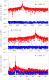 |
Fig. D.1 Numerical errors on the computation of ∂rεℬ using double precision arithmetic. The red curve shows the relative error obtained when using Eq. (D.2); the blue curve shows the relative error obtained when using Eq. (D.3). Errors are computed from a reference value obtained in quadruple precision. Panel a, b, and c show the error as a function of the distance r of the particle for the Orbits #1, #2, and #3 considered in Sect. 6, with parametrisation point q = r⋆. The values of r shown range from periapsis to apoapsis. |
Figure D.1 compares the results obtained when using the direct difference in Eq. (D.2) or the factored expression in Eq. (D.3). The red curve in panels a and b show a clear peak at r ≈ q, where errors are maximum. These errors are absent in the blue curve, which always remain near machine precision. The red curve in panel c features two peaks: the first peak arises near r = q, and it is corrected on the blue curve. The second peak arises near r = rc.
Only the first set of coefficients given by Kinoshita et al. (1990), referred to as SI6A, is implemented in galpy.
The question whether symplectic integrators are advantageous in the context of galactic dynamics is a recurring debate. We consider they are (e.g. because systematic variations in energy would irremediably bias statistics computed on many trajectories); however, taking part in this debate is not our aim here.
If needed in this particular case, close encounters between stars can be modelled independently as small stochastic impulses.
We used the convention for the Poisson bracket: {f, g} = ∂qf · ∂pg − ∂pf · ∂qg.
What we call ‘energy drift’ is an irreversible variation in energy produced by the non-zero error terms inherent to the integration method. This variation can be made to remain below machine precision (in which case the remaining variations in energy are only due to numerical round-off errors), but this requires using a small enough time step.
𝒮𝒜ℬ𝒜1 corresponds to the Leapfrog integration scheme.
In practice, as we want |εℬ| to be as small as possible, we must take care of the dramatic cancellation errors generated by the difference in Eq. (33) by implementing the equation in a cancellation-safe way (see Appendix D).
Specifically, the adopted values were taken from the edition available at https://people.smp.uq.edu.au/HolgerBaumgardt/globular/parameter.html as of September 30, 2024.
By definition, we always have α ≥ b for a bounded orbit.
All Tables
All Figures
|
Fig. 1 Maximum relative variation in the Hamiltonian in Eq. (29) as a function of the time step used. We integrate a slightly perturbed isochrone potential where ε = 10−4. The integration is conducted over two radial periods (Δt = 2τ ≈ 239) of an orbit with unperturbed isochrone semi-major axis α ≈ 7.12 and eccentricity ε ≈ 4.21 × 10⁻¹. Black lines show several power laws for comparison. |
| In the text | |
|
Fig. 2 Relative error in total energy as a function of time for the same orbit as in Fig. 1. The behaviour of two fourth-order integrators is shown: the Runge-Kutta method and the 𝒮𝒜ℬ𝒜2 method using the isochrone splitting (see the labels). A constant time step δt = 2.5 is used for both integrators. |
| In the text | |
|
Fig. 3 Value of the Hamiltonian εℬq(r) in Eq. (35) as a function of the parametrisation point, q, and the star’s instantaneous position, r. The value of εℬq(r) is shown by the colour shades and black level curves. By definition of q, the value of εℬq(r) is zero along the diagonal (i.e. for r = q). An example of the periapsis, rp, apoapsis, ra, and best parametrisation point, q⋆, are shown in red and blue. In this system of units, the Plummer characteristic radius, κ, lies at r = 1. |
| In the text | |
|
Fig. 4 Optimal parametrisation point, q⋆, as a function of the periapsis and apoapsis of the orbit. Some level curves appear in white. Regions I, II, and III are described in the text. |
| In the text | |
|
Fig. 5 Size, E⋆, of the perturbation (panel a) and relative magnitude, ε⋆, of the perturbation (panel b) computed for the optimal parametrisation point, q⋆. Some level curves appear in black. The three coloured points were used for the numerical experiments described in Sect. 6 (see Figs. 7 and 8). |
| In the text | |
|
Fig. 6 Size, E, of the perturbation computed for q = rp (panel a) and q = ra (panel b) compared to the best parametrisation point, q⋆. The colour scale in panel a is linear; the colour scale in panel b is logarithmic. The level curve Ea/E⋆ = 10 is shown in white. The three coloured points were used for the numerical experiments described in Sect. 6 (see Figs. 7 and 8). |
| In the text | |
|
Fig. 7 Maximum relative variation in the Hamiltonian as a function of the integration time step over the radial period (top row) and as a function of the CPU integration time (bottom row). Each column corresponds to a different orbit (orange, red, and green points in Figs. 5 and 6), integrated over two radial periods with 𝒮𝒜ℬ𝒜1. The blue curve and the black curve show the results obtained when using kinetic splitting and Kepler splitting. The orange, green, and pink curves correspond to the isochrone splitting with parametrisation points q = rp, q = ra, and q = r⋆, respectively. |
| In the text | |
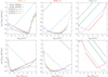 |
Fig. 8 Same as Fig. 7 but using the 𝒮𝒜ℬ𝒜3 integrator. |
| In the text | |
|
Fig. 9 Maximum relative variation in the Hamiltonian as a function of the parameters μ and b of the isochrone potential used for the splitting. Each column corresponds to a different orbit (orange, red, and green points in Figs. 5 and 6), integrated with 𝒮𝒜ℬ𝒜1 over two radial periods for a given integration time step, δt. The orange, green, and pink points correspond to the isochrone splitting with parametrisation points q = rp, q = ra, and q = r⋆, respectively (the points overlap for Orbit #2), while the cyan curve shows all possible parametrisation points, q, between the periapsis distance and apoapsis distance, following Eq. (34). |
| In the text | |
|
Fig. A.1 Example of a particle’s motion in its orbital plane (a special case of a closed orbit where Δφ = 3π/2) with the isochrone parameters μ = 1 and b = 2 × 10⁻¹. The green and blue circles, labelled Crp and Cra, respectively show the particle’s minimum and maximum radial positions. The dashed violet line, denoted by r(t), shows the particle’s orbit. The solid violet line shows the path of the particle during one radial period; its length is given by Γ (see Eq. (A.4)). The small arrow indicates the rotational sense of the loops. |
| In the text | |
|
Fig. D.1 Numerical errors on the computation of ∂rεℬ using double precision arithmetic. The red curve shows the relative error obtained when using Eq. (D.2); the blue curve shows the relative error obtained when using Eq. (D.3). Errors are computed from a reference value obtained in quadruple precision. Panel a, b, and c show the error as a function of the distance r of the particle for the Orbits #1, #2, and #3 considered in Sect. 6, with parametrisation point q = r⋆. The values of r shown range from periapsis to apoapsis. |
| In the text | |
Current usage metrics show cumulative count of Article Views (full-text article views including HTML views, PDF and ePub downloads, according to the available data) and Abstracts Views on Vision4Press platform.
Data correspond to usage on the plateform after 2015. The current usage metrics is available 48-96 hours after online publication and is updated daily on week days.
Initial download of the metrics may take a while.