| Issue |
A&A
Volume 628, August 2019
|
|
|---|---|---|
| Article Number | A32 | |
| Number of page(s) | 13 | |
| Section | Planets and planetary systems | |
| DOI | https://doi.org/10.1051/0004-6361/201935786 | |
| Published online | 31 July 2019 | |
High-order regularised symplectic integrator for collisional planetary systems
ASD/IMCCE, CNRS-UMR8028, Observatoire de Paris, PSL University, Sorbonne Université,
77 avenue Denfert-Rochereau,
75014
Paris,
France
e-mail: This email address is being protected from spambots. You need JavaScript enabled to view it.
Received:
26
April
2019
Accepted:
15
June
2019
Abstract
We present a new mixed variable symplectic (MVS) integrator for planetary systems that fully resolves close encounters. The method is based on a time regularisation that allows keeping the stability properties of the symplectic integrators while also reducing the effective step size when two planets encounter. We used a high-order MVS scheme so that it was possible to integrate with large time-steps far away from close encounters. We show that this algorithm is able to resolve almost exact collisions (i.e. with a mutual separation of a fraction of the physical radius) while using the same time-step as in a weakly perturbed problem such as the solar system. We demonstrate the long-term behaviour in systems of six super-Earths that experience strong scattering for 50 kyr. We compare our algorithm to hybrid methods such as MERCURY and show that for an equivalent cost, we obtain better energy conservation.
Key words: celestial mechanics / planets and satellites: dynamical evolution and stability / methods: numerical
© A. C. Petit et al. 2019
 Open Access article, published by EDP Sciences, under the terms of the Creative Commons Attribution License (http://creativecommons.org/licenses/by/4.0), which permits unrestricted use, distribution, and reproduction in any medium, provided the original work is properly cited.
1 Introduction
Precise long-term integration of planetary systems is still a challenge today. The numerical simulations must resolve the motion of the planets along their orbits, but the lifetime of a system is typically billions of years, resulting in computationally expensive simulations. In addition, because of the chaotic nature of planetary dynamics, statistical studies are often necessary, which require running multiple simulations with close initial conditions (Laskar & Gastineau 2009). This remark is particularly true for unstable systems that can experience strong planet scattering caused by close encounters.
There is therefore considerable interest in developing fast and accurate numerical integrators, and numerous integrators have been developed over the years to fulfill this task. For long-term integrations, the most commonly used are symplectic integrators. Symplectic schemes incorporate the symmetries of Hamiltonian systems, and as a result, usually conserve the energy and angular momentum better than non-symplectic integrators. In particular, the angular momentum is usually conserved up to a roundoff error in symplectic integrators.
Independently, Kinoshita et al. (1991) and Wisdom & Holman (1991) developed a class of integrators that are often cal- led mixed variable symplectic (MVS) integrators. This method takes advantage of the hierarchy between the Keplerian motion of the planets around the central star and the perturbations indu- ced by planet interactions. It is thus possible to make accurate integrations using relatively large time-steps.
The initial implementation of Wisdom & Holman (1991) is a low-order integration scheme that still necessitates small time-steps to reach machine precision. Improvements to the method have since been implemented. The first category is symplectic correctors (Wisdom et al. 1996; Wisdom 2006). They consist of a modification of the initial conditions to improve the scheme accuracy. Because it is only necessary to apply them when an output is desired, they do not affect the performance of the integrator. This approach is for example used in WHFAST (Rein & Tamayo 2015). The other approach is to consider higher order schemes (McLachlan 1995b; Laskar & Robutel 2001; Blanes et al. 2013). High-order schemes permit a very good control of the numerical error by fully taking advantage of the hierarchical structure of the problem. This has been used with success to carry out high-precision long-term integrations of the solar system (Farrés et al. 2013).
The principal limitation of symplectic integrators is that they require a fixed time-step (Gladman et al. 1991). If the time-step is modified between each step, the integrator remains symplectic because each step is symplectic. However, the change in time-step introduces a possible secular energy drift that may reduce the interest of the method. As a consequence, classical symplectic integrators are not very adapted to treat the case of systems that experience occasional close encounters where very small time-steps are needed.
To resolve close encounters, Duncan et al. (1998) and Chambers (1999) provided solutions in the form of hybrid symplectic integrators. Duncan et al. (1998) developed a multiple time-step symplectic integrator, SYMBA, where the smallest time-steps are only used when a close encounter occurs. The method is limited to an order two scheme, however. The hybrid integrator MERCURY (Chambers 1999) moves terms from the perturbation step to the Keplerian step when an interaction between planets becomes too large. The Keplerian step is no longer integrable but can be solved at numerical precision using a non-symplectic scheme such as Burlisch–Stoer or Gauss–Radau. However, the switch of numerical method leads to a linear energy drift (Rein & Tamayo 2015). Another solution to the integration of the collisional N-body problem has been proposed in (Hernandez & Bertschinger 2015; Hernandez 2016; Dehnen & Hernandez 2017). It consists of a fixed time-step second-order symplectic integrator that treats every interaction between pairs of bodies as Keplerian steps.
Another way to build a symplectic integrator that correctly regularises close encounters is time renormalisation. Up to an extension of the phase space and a modification of the Hamiltonian, it is indeed always possible to modify the time that appears in the equations of motion. As a result, the real time becomes a variable to integrate. Providing some constraints on the renormalisation function, it is possible to integrate the motion with a fixed fictitious time-step using an arbitrary splitting scheme. Here we show that with adapted time renormalisation, it is possible to resolve close encounters accurately.
While time renormalisation has not been applied in the context of close encounters of planets, it has been successful in the case of perturbed highly eccentric problems (Mikkola 1997; Mikkola & Tanikawa 1999; Preto & Tremaine 1999; Blanes & Iserles 2012), see Mikkola (2008) for a general review. We here adapt a time renormalisation proposed independently by Mikkola & Tanikawa (1999) and Preto & Tremaine (1999). We show that it is possible to use the perturbation energy to monitor close encounters in the context of systems with few planets with similar masses. We are able to define a MVS splitting that can be integrated with any high-order scheme.
We start in Sect. 2 by briefly recalling the basics of the symplectic integrator formalism. In Sect. 3 we present the time renormalisation that regularises close encounters, and we then discuss the consequence of the renormalisation on the hierarchical structure of the equations (Sect. 4). In Sect. 5 we numerically demonstrate over short-term integrations the behaviour of the integrator at close encounter. We then explain (Sect. 6) how our time regularisation can be combined with the perihelion regular isation proposed by Mikkola (1997). Finally, we show the results of long-term integration of six planet systems in the context of strong planet scattering (Sect. 7) and compare our method to a recent implementation of MERCURY described in Rein et al. (2019), to SYMBA, and to the non-symplectic high-order integrator IAS15 (Sect. 8).
2 Splitting symplectic integrators
We consider a Hamiltonian H(p, q) that can be written as a sum of two integrable Hamiltonians,
 (1)
(1)
A classical example is given by H0 = T(p) and H1 = U(q), where T(p) is the kinetic energy and U(q) is the potential energy. In planetary dynamics, we can split the system as H0 = K(p, q), where K is the sum of the Kepler problems in Jacobi coordinates (e.g. Laskar 1990) and H1 = Hinter(q) is the interaction between the planets.
Using the Lie formalism (e.g. Koseleff 1993; Laskar & Robutel 2001), the equation of motion can be written
 (2)
(2)
where z = (p, q), {⋅, ⋅} is the Poisson bracket1, and we note Lf = {f, ⋅}, the Lie differential operator. The formal solution of Eq. (2) at time t = τ+ t0 from the initial condition z(t0) is
 (3)
(3)
In general, the operators  and
and  do not commute, sothat
  However, using the Baker-Campbell-Hausdorff (BCH) formula, we can find the coefficients ai and bi such that
 (4)
(4)
where Herr = O(τr) is an error Hamiltonian depending on H0, H1, τ and the coefficients ai and bi.
Because H0 and H1 are integrable, we can explicitly compute the evolution of the coordinates z under the action of the maps  and
and  . The map
  is symplectic because it is a composition of symplectic maps. Moreover,
  exactly integrates the Hamiltonian H + Herr.
If there is a hierarchy in the Hamiltonian H in the sense that |H1 ∕ H0|≃ ε ≪ 1, we can choose the coefficients such that the error Hamiltonian is of the order of
 (5)
(5)
(see McLachlan 1995b; Laskar & Robutel 2001; Blanes et al. 2013; Farrés et al. 2013). For small ε and τ, the solution of H + Herr is very close to the solution of H. In particular, it is thought that the energy error of a symplectic scheme is bounded. Because Herr depends on τ, a composition of steps  also has thisproperty if the time-step is kept constant. Otherwise, the exact integrated dynamics changes at each step, leading to a secular drift of the energy error.
In planetary dynamics, we can split the Hamiltonian such that H0 is the sum of the Keplerian motions in Jacobi coordinates and H1 is the interaction Hamiltonian between planets, which only depends on positions and thus is integrable (e.g. Laskar 1990). This splitting naturally introduces a scale separation ε given by
 (6)
(6)
where N is the number of planets, mk is the mass of the kth planet, and m0 is the mass of the star. If the planets remain far from each other, H1 is always ε small with respect to H0.
The perturbation term is of the order of ε ∕ Δ, where Δ is the typical distance between the planets in units of a typical length of the system. During close encounters, Δ can become very small, and the step size needs to be adapted to ε ∕ Δmin Here Δmin is the smallest expected separation between planets normalised by a typical length of the system.
3 Regularised Hamiltonian
3.1 General expression
In order to construct an adaptive symplectic scheme that regularises the collisions, we extend the phase space and integrate the system with a fictitious time. Let s be such that
 (7)
(7)
where g is a function to be determined and pt is the conjugated momentum to the real time t in the extended phase space. In order to have an invertible function t(s), we require g to be positive. We consider the new Hamiltonian Γ defined as
 (8)
(8)
Γ does not depend on t, therefore pt is a constant of motion. The equations of motion of this Hamiltonian are
 (9)
(9)
and for all function f(z)
 (10)
(10)
In general, H is not a constant of motion of Γ. We have
 (11)
(11)
If we choose initial conditions z0 such that pt = −H(z0), we have  . Because Γ is constant and g is positive, we deduce from Eq. (3) that we have at all times
 (12)
(12)
Because pt is also a constant of motion, H is constant for all times. We can simplify the Eqs. of motion (9) and (10) into
 (13)
(13)
On the manifold pt = −H(t0), Eq. (13) describe the same motion as Eq. (2). We call them the regularised equations.
We now wish to write Γ as a sum of two integrable Hamiltonians such as in Sect. 2. Based on previous works (Preto & Tremaine 1999; Mikkola & Tanikawa 1999; Blanes & Iserles 2012), we write
 (14)
(14)
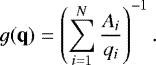
for H = H0 + H1 and we define g as
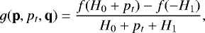 (15)
(15)
where f is a smooth function to be determined. g is the difference quotient of f and is well defined when H0 + pt + H1 → 0. We have
 (16)
(16)
With this choice of g, the Hamiltonian Γ becomes
 (17)
(17)
where we note Γ0 = f(H0 + pt) and Γ1 = −f(−H1). We remark that Γ0 (resp. Γ1) is integrable because it is a function of H0 + pt (resp. H1), which is integrable. Moreover, we have
 (18)
(18)
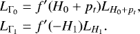
Because H0 + pt (resp. H1) is a first integral of Γ0 (resp. Γ1), we have
 (19)
(19)
where
 (20)
(20)
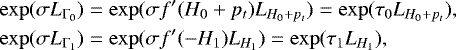
The operator  (
(  ) is equivalent to the regular operator
  (
(  ) with a modified time step. The operator exp(σLΓ) can be approximated by a composition of operators
 (21)
(21)
With the BCH formula,  where Γerr is an error Hamiltonian that depends on σ. The symplectic map
  exactly integrates the modified Hamiltonian Γ + Γerr. The iteration of
  with fixed σ is a symplectic integrator algorithm for Γ.
When the timescale σ is small enough, the numerical values of H0 and H1 do not change significantly between each step of the composition. We have  with τ ≃ σf ′(−H1). In other words,
  behaves as
  with an adaptive time-step while keeping the bounded energy properties of a fixed time-step integrator.
3.2 Choice of the regularisation function
We wish thestep sizes (20) to become smaller when planets experience close encounters. These time-steps are determined by the derivative of f. For nearly Keplerian systems, Mikkola & Tanikawa (1999) and Preto & Tremaine (1999) studied renormalisation functions such that f′ (x) ∝ x−γ, where γ > 0 (this corresponds to power-law functions and the important case of f = ln).
However, these authors considered splitting of the type H0 = T(p) and H1 = U(q). As pointed out in Blanes & Iserles (2012), when the Hamiltonian is split as the Keplerian part plus an integrable perturbation, it appears that both terms K(p, q) + pt and − H1 can change signs, resulting in large errors in the integration.
We remark that the use of f = ln gives the best result when two planets experience a close encounter, but it leads to large energy errors far away for collision when H1 is nearly 0. Based on these considerations, we require f to verify several properties to successfully regularise the perturbed Keplerian problem in presence of close encounters:
-
f ′ should only depend on the magnitude of the perturbation H1, thereforewe require f ′ even (and f odd).
As already pointed out, t must be an increasing function of s, therefore f ′ > 0.
f ′ should be smooth, therefore we exclude piecewise renormalisation functions.
We require that the regularisation vanishes in absence of perturbation i.e. f′(0) = 1. It results that for vanishing perturbation, σ = τ.
Let E1 be a typical value of H1 far from close encounters that we determine an expression for below. f′ should only depend on H1∕E1 in order to only track relative changes in the magnitude of the perturbation.
For high values of the perturbation (e.g. during close encounters), we require f ′(H1) ~|E1∕H1| such that we preserve the good properties pointed out by previous studies (Preto & Tremaine 1999; Mikkola & Tanikawa 1999).
To reduce the computational cost of the integrator, f ′ has to be numerically inexpensive to evaluate.
These properties lead to a very natural choice for f ′ (see in Fig. 1). We choose
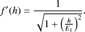 (22)
(22)
Taking the odd primitive of Eq. (22), we find
 (23)
(23)
For now on, f always refers to definition (23). With this choice of the function f, the Hamiltonian Γ takes the form
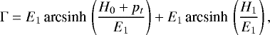 (24)
(24)
where we used the oddity of f.
We need to define E1 more explicitly. When planets are far from each other, their mutual distance is of the same order as the typical distance between the planets and the star. Using the same idea as in Marchal & Bozis (1982); Petit et al. (2018), we define a typical length unit of the system based on the initial system energy E0. We have
 (25)
(25)
where M * = ∑0≤i<jmimj. The typical value for the perturbation Hamiltonian far away from collision can be defined as
 (26)
(26)
where m* = ∑1≤i<jmimj. We note that we have E1 ∕ E0 = O(ε).
The behaviour of the higher order derivative of f is useful for the error analysis, and in particular, their dependence in ε. The kth derivative of f has for expression
 (27)
(27)
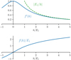 |
Fig. 1 Upper panel: f ′, Eq. (22) as a function of h∕E1. The asymptotic value for h∕E1 → +∞ is given in green. Lower panel: f∕E1, Eq. (23) as a function of h∕E1. |
4 Order of the scheme
4.1 Analytical error estimates
As explained in Sect. 2, most of the planet dynamics simulations are made with a simple a second-order scheme such as the Wisdom–Holman leapfrog integrator (Wisdom & Holman 1991). It is indeed possible to take advantage of the hierarchy between H0 and H1. This can be done by adding symplectic correctors (Wisdom et al. 1996; Rein & Tamayo 2015) or by cancelling the term of the form ετk up to a certain order (Laskar & Robutel 2001).
Hierarchical order schemes such as  (Blanes et al. 2013; Farrés et al. 2013) behave effectively as a tenth-order integrator if ε is small enough. Cancelling only selected terms reduces the number of necessary steps of the scheme, which reduces the numerical error and improves the performances.
Unfortunately, this property cannot be used for the regularised Hamiltonian because Γ0 and Γ1 are almost equal in magnitude. Nevertheless, it should be noted that the equations of motion (13) and the Lie derivatives (18) keep their hierarchical structure. The Poisson bracket of Γ0 and Γ1 gives
 (28)
(28)
Because f′ does not depend directly on ε (by choice, f′ only tracks relative variations of H1), {Γ0, Γ1} is of the order of ε. However, for higher order terms in σ in Herr, it is not possible to exploit the hierarchical structure in ε. We consider the terms of the order of σ2 in the error Hamiltonian for the integration of Γ using the leapfrog scheme. We have (e.g. Laskar & Robutel 2001)
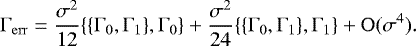 (29)
(29)
In order to show the dependence in ε, we develop the Poisson brackets in Eq. (29)
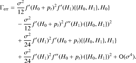 (30)
(30)
The first and third terms only depend on f′ and nested Poisson brackets of H0 and H1. Their dependency on ε is thus determined by the Poisson brackets as in the fixed time-step case. The first term is of the order of εσ2 and the third of the order of ε2σ2. On the other hand, the second and last terms introduce the second derivative of f as well as a product of Poisson bracket of H0 and H1. Equation (27) shows that they are of the order of εσ2.
In order to cancel all terms of the order of εσ2, it is necessary to cancel both terms by σ2 in Eq. (29). Thus, the strategy used in Blanes et al. (2013) does not provide a scheme with a hierarchical order because every Poisson bracket contributes with terms of the order of ε to the error Hamiltonian.
It is easy to extend the previous result to all orders in σ. We consider a generic error term of the form
 (31)
(31)
where kj is either 0 or 1 and k0 = 0 and k1 = 1. The development of Γgen into Poisson brackets of H0 and H1 contains a term that has for expression
 (32)
(32)
where nj is the number of Γj in Γgen, and  . Because n = n0 + n1, we deduce from Eq. (27) that the term Eq. (32) is of the order of εσn−1. Thus, the effective order of the Hamiltonian is always εσrmin, where rmin is the smallest exponent rk in Eq. (5). The error is still linear in ε. Hence, it is still worth using the Keplerian splitting.
We useschemes that are not dependent on the hierarchy between H0 and H1. McLachlan (1995a) provided an exhaustive list of the optimal methods for fourth-, sixth-, and eighth-order integrators. Among the schemes he presented, we select a sixth-order method consisting of a composition of n =7 leapfrog steps introduced by Yoshida (1990) and an eighth-order method that is a combination of n =15 leapfrog steps. A complete review of these schemes can be found in Hairer et al. (2006). The coefficients of the schemes are given in Appendix B.
In order to solve the Kepler step, we adopt the same approach as Mikkola (1997); Rein & Tamayo (2015). The details on this particular solution as well as other technical details are given in Appendix A.
4.2 Non-integrable perturbation Hamiltonian
When the classical splitting of the Hamiltonian written in canonical heliocentric coordinates is used, H1 depends on both positions and momenta. We can write H1 as a sum of two integrable Hamiltonian H1 = T1 + U1, where T1 is the indirect part that only depends on the momenta and U1 is the planet interaction potential, only depending on positions (Farrés et al. 2013). We thus approximate the evolution operator (19) by
 (33)
(33)
The numerical results suggest that heliocentric coordinates give slightly more accurate results at constant cost. It is possible to use an alternative splitting that is often called democratic heliocentric splitting (Laskar 1990; Duncan et al. 1998). With this partition of the Hamiltonian, the kinetic and the potential part of the perturbation Hamiltonian commute. Therefore, the step  is directly integrable using the effective step size τ1 Eq. (20). In the following numerical tests, we always use the classical definition when we refer to heliocentric coordinates.
5 Error analysis near the close encounter
5.1 Time-step and scheme comparison
In this section, we test how a single close encounter affects the energy conservation. To do so, we compare different integration schemes for a two-planet system, initially on circular orbits, during an initial synodic period
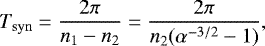 (34)
(34)
where ni is the mean motion of planet i and α is the ratio of the semi-major axis.
Because the time-step is renormalised, we need to introduce a cost function that depends on the fictitious time s as well as on the number of stages involved in the scheme of the integrator. We define the cost of an integrator as the number of evaluations of  that are required to integrate for a given real time period Tsyn
 (35)
(35)
where ssyn is the fictitious time after Tsyn, σ is the fixed fictitious time-step, and n is the number of stages of the integrator. We also compare the renormalised integrators to the same scheme with fixed time-step. For a fixed time-step, the cost function is simply given by  , where τ is the time-step (Farrés et al. 2013). We present different configurations in Figs. 2–4.
In the two first sets, we integrate the motion of two equal-mass planets on circular orbits, starting in opposition with respect to the star. In both simulations, we have ε = (m1 + m2)∕m0 = 10−5, the stellar mass is 1 M⊙, and the outer planet semi-major axis is 1 AU. In both figures, we represent the averaged relative energy variation
 (36)
(36)
as a function of the inverse cost  of the integration for various schemes:
-
the classical order 2 leapfrog
 ,
, -
the scheme
 from Laskar & Robutel (2001),
 -
the scheme
 from Blanes et al. (2013),
 -
the sixth- and eighth-order schemes from McLachlan (1995a) that we introduced in the previous section.
For each scheme, we plot with a solid line the result of the fixed time-step algorithm and with dots the results of the adaptive time-step integrator. In the results presented in Figs. 2 and 3, the systems are integrated in Jacobi coordinates. In Fig. 4 we integrate in heliocentric coordinates. For the three cases, the integrations were also carried out with the other set of coordinates with almost no differences.
In Fig. 2 the initial semi-major axis ratio α is 0.8 and the closest approach of the two planets is 0.19992 AU. In this case, a fixed time-step algorithm provides accurate results, and when a generalized order scheme suchas  or
or  is used, the performances are better with a fixed time-step than with an adaptive one. However, we see no sensitive differences in accuracy between the fixed and adaptive versions of the
  and
and  schemes. For the most efficient schemes, machine precision is reached for an inverse cost of a few 10−3. This case illustrates the point made in Sect. 4 that there is no advantage in using the hierarchical structure of the original equation in the choice of the scheme.
In Fig. 3 the initial semi-major axis ratio α is 0.97 and the closest approach of the two planets is 3.68 × 10⁻⁵ AU. The radius of a planet of mass 5 × 10⁻⁶ M⊙ with a density of 5 g cm−3, denser than Earth, is 5.21 × 10⁻⁴ AU, that is, ten times greater. We can compute the density that corresponds to a body of mass 5 × 10⁻⁶ M⊙ and radius half the closest approach distance. Weobtain a density of 1.1 × 10⁵ g cm−3, which is close to the white dwarf density. In this case, the fixed time-step algorithm is widely inaccurate while the performance of the adaptive time-step algorithm remains largely unchanged. This demonstrates how powerful this new approach is for the integration of systems with a few planets.
We also give an example with higher mass planets in Fig. 4. We plot the relative energy error as a function of the inverse cost for a system of two planets of mass 5 × 10⁻⁴ M⊙ that correspond to the case of ε = 10−3. The initial semi-major axis ratio is 0.9 to ensure a closest-approach distance of 1.7 × 10⁻² AU.
For this particular close encounter, it is still possible to reach machine precision with a fixed time-step at the price of a very small time-step. On the other hand, the close encounter is perfectly resolved for the adaptive time-step, even if ε is larger by two orders of magnitude. Because of the higher masses, it is necessary to take smaller time-steps to ensure that the relative energy error remains at machine precision.
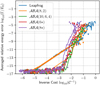 |
Fig. 2 Comparison between various schemes detailed in the body of the text for the integration of a single synodic period for a system of equal-mass planets initially on planar circular orbits with ε = 2m∕m0 = 10−5 and α = 0.8. The solid lines represent the integrations using a fixed real time-step and the dots the adaptive time-steps. The closest planet approach is 0.19992 AU. |
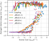 |
Fig. 3 Same as Fig. 2 for a system of two equal-mass planets initially on planar circular orbits with ε = 2m∕m0 = 10−5 and α = 0.97. The closest planet approach is 3.68 × 10⁻⁵ AU. |
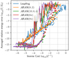 |
Fig. 4 Same as Fig. 2 for a system of two equal-mass planets initially on planar circular orbits with ε = 2 m∕m0 = 10−3 and α = 0.9. The closest planet approach is 1.7 × 10⁻² AU. This systemis integrated in heliocentric coordinates to demonstrate that we obtain similar results to the case of Jacobi coordinates. |
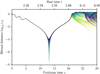 |
Fig. 5 Mutual distance of the planets as a function of the fictitious time for 1000 initial conditions chosen as described in the body of the text. On the upper axis, we give the real time for the initial condition that reached the closest approach. |
5.2 Behaviour at exact collision
To demonstrate the power of our algorithm in resolving close encounters, we considered the case of two planets thatalmost exactly collide (as if the bodies were material points). We take two planets of mass m = 10−5 M⊙, the first on an orbit of eccentricity 0.1 and semi-major axis 0.95 AU, and the second on a circular orbit of semi-major axis 1 AU. We then fine-tuned the mean longitudes of the two planets to ensure that we approach the exact collision. We integrated 1000 initial conditions for which we linearly varied λ1 between −0.589 and −0.587, and we took λ2 = −1.582.
In Fig. 5 we represent for each initial condition the mutual distance of the planets as a function of the fictitious time s. In the upper axis, we give the real time of the particular initial condition that gave the closest approach. In this simulation, all initial conditions reached a mutual distance smaller than 1.1 × 10⁻⁴ AU and the closest approach is 5.5 × 10⁻⁹ AU. For the chosen masses, we can compute the physical radius of such bodies assuming a particular bulk density. We have
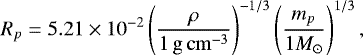 (37)
(37)
where ρ is the bulk density of the planet. The radius is only a weak function of the density over the range of planet bulk densities. When we assume a very conservative value of ρ = 6 g cm−3, we obtain a planet radius of 6.17 × 10⁻⁴ AU, that is, well above the close encounters considered here.
We plot the energy error as a function of the closest approach distance in Fig. 6. We also considered a more practical case where four other planets were added to the system. The additional planets were located on circular orbits, had the same masses of 10−5 M⊙ and were situated outside of the orbit of the second planet, with an equal spacing of 0.15 AU. Their initial angles are randomly drawn but were similar in every run.
In both set-ups, we used the heliocentric  scheme, and the fictitious time-step was σ = 10−2. In the case of the two-planet system, machine precision is reached even for an approach of approximately 10−6 AU, which corresponds to a planet radius of about 10−3. When planets are added, it is more difficult to reach very close encounters because the other planets are perturbed. Nonetheless, approaches up to 6 × 10⁻⁷ AU are reached,and the close encounter is resolved at machine precision up to a closest distance of 3 × 10⁻⁵ AU or a planet radius of 5 × 10⁻².
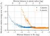 |
Fig. 6 Relative energy error as a function of the closest mutual approach reached during a close encounter of super-Earths in a two-planet system and in a six-planet system. The particular initial conditions are described in the text. In the upper part, we give the mutual distance in units of planet radii for a planet of density ρ = 6 g cm−3. |
6 Pericenter regularisation
When planet–planet scattering is studied, the closest distance between the planet and the star may be reduced. As a result, the fixed time-step becomes too large and the passage at pericenter is insufficiently resolved. In order to address this problem, we can combine theclose-encounter regularisation of Sect. 3 with a regularisation method introduced by Mikkola (1997).
We firstdetail Mikkola’s idea. When integrating a few-body problem Hamiltonian, a time renormalisation d t = g(q)du can be introduced, where
 (38)
(38)
Here Ai are coefficients that can be chosen arbitrarily. In this article, we define them as
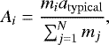 (39)
(39)
where atypical, defined in Eq. (25), is the typical length scale of the system. The new Hamiltonian ϒ in the extended phase space (q, t, p, pt) is
 (40)
(40)
As in Sect. 3, in the sub-manifold {pt = H(0)}, ϒ and H have the same equations of motion up to the time transformation. If H1 only depends on q (using Jacobi coordinates, e.g.), ϒ1 is trivial to integrate.
6.1 Kepler step
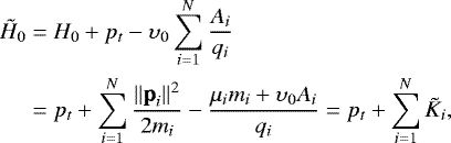
It is also possible to integrate ϒ0 as a modified Kepler motion through the expression of g (Mikkola 1997). We denote υ0 = ϒ0(0) and 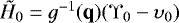 .
.  has the same equations of motion asϒ0 up to a time transformation
  . We have
 (41)
(41)
where  is the Hamiltonian of a Keplerian motion of planet i with a modified central mass
 (42)
(42)
However, the time equation must be solved as well. We integrate with a fixed fictitious time-step Δu. The time  is related to u through the relation
 (43)
(43)
where  follows a Keplerian motion. We can rewrite Eq. (43) with the Stumpff formulation of the Kepler equation (Mikkola 1997; Rein & Tamayo 2015, see Appendix A.1). Because
  , we have
 (44)
(44)
As a consequence, the N Stumpff–Kepler equations
 (45)
(45)
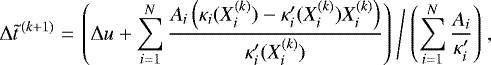
must be solved simultaneously with Eq. (44). To do so, we used a multidimensional Newton-Raphson method on the system of N + 1 equations consisting of the N Kepler Eqs. (45) and (44) of unknowns  . The algorithm is almost as efficient as the fixed-time Kepler evolution because it does not add up computation of Stumpff’s series. At step k, we can obtain Y(k+1) through the equation
 (46)
(46)
where
![Mathematical equation: \begin{equation*} F = \left(\begin{array}{c} \kappa_1(X_1)-\Delta\tilde t\\ \vdots\\ \kappa_N(X_N)-\Delta\tilde t\\[3pt] \sum_{i=1}^{N}A_iX_i-\Delta u \end{array}\right), \end{equation*}](/articles/aa/full_html/2019/08/aa35786-19/aa35786-19-eq89.png) (47)
(47)
and
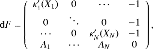 (48)
(48)
with  being the derivative with respect to Xi of κi (Eq. (45)).
Equation (46) can be rewritten as a two-step process where a new estimate for the time  is computed and is then used to estimate
  . We have
 (49)
(49)
and
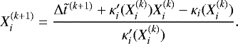 (50)
(50)
6.2 Heliocentric coordinates
In heliocentric coordinates,  depends on p as well. As a result,
  cannot be easily integrated, and it is not even possible write it as a sum of integrable Hamiltonians. To circumvent this problem, we can split
  into
into  and
and  . The potential part
  is integrable, but a priori,
  is not integrable.
The integration of  can be integrated using a logarithmic method as proposed in Blanes & Iserles (2012). The evolution of
  during a step Δt is the same as the evolution of
  , which is separable, for a step
  where
where  . Therefore, we can approximate
  using a leapfrog scheme, and the error is of order Δu2ε3 as well.
Then, we can approximate the heliocentric step using the same method as in Sect. 4.2. In this case, it is necessary to approximate the step even when democratic heliocentric coordinates are used because g(q) does not commute with  .
.
6.3 Combining the two regularisations
We showed that the Hamiltonian ϒ is separable into two parts that are integrable (or nearly integrable for heliocentric coordinates). Therefore we can simply regularise the close encounters by integrating the Hamiltonian
 (51)
(51)
where pu is the momentum associated with the intermediate time u used to integrate ϒ alone. The time equation is
 (52)
(52)
We need to place ourselves on the sub-manifold such that ϒ0 + pu + ϒ1 = 0 and H0 + pt + H1 = 0, in order to have the same equations of motion for  , ϒ and H. Both of these conditions are fulfilled by choosing pt = −E0 and pu = 0.
7 Long-term integration performance
So far, we only presented the performance of the algorithm for very short integrations. In this section, we present the long-term behaviour of the integrator for systems with a very chaotic nature. We consider two different configurations, a system composed of equal planet masses on initially circular, coplanar and equally spaced orbits, used as a test model for stability analysis since the work of Chambers et al. (1996). The second is a similar system but with initially moderate eccentricities and inclinations.
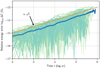 |
Fig. 7 Evolution of the relative energy error for 100 systems composed of six planets on initially circular orbits. The light curves represent individual systems, and the thicker blue curves show the average over the 100 systems. The orange straight line is proportional to
|

7.1 Initially circular and coplanar systems
We integrated 100 systems of six initially coplanar and circular planets. The planet masses were taken to be equal to 10−5 M⊕, and the semi-major axis of the outermost planet was fixed to 1 AU, while the semi-major axis ratios of the adjacent planets were all equal to 0.88. These valus were chosen to ensure that the lifetime of the system was of the order of 300 kyr before the first collision. The fixed fictitious time-step was σ = 10−2 yr. Because of the renormalisation, this approximately corresponds to a fixed time-step of 6.3 × 10⁻³ yr in terms of computational cost. The initial period of the inner planet was of the order of 0.38 yr, that is, we have about 50 steps per orbit.
The simulations were stopped when two planet centres approached each other by less than half the planet radii, assuming a density of 6 g cm−3. This stopping criterion is voluntarily nonphysical as it allows for a longer chaotic phase that leads to more close encounters. We also monitored any encounters with an approach closer than 2 Hill radii at 1 AU (0.054 AU) and recorded its time, the planets involved, and the closest distance between the two planets.
For the majority of the integrations, we observe moderate semi-major axis diffusion without close encounters. About 1 kyr before the final collision, the system enters a true scattering phase with numerous close encounters. The integrations lasted on average 353 kyr, the shortest was 129 kyr long and the longest 824 kyr. On average, we recorded 557 close encounters, and 68% occurred during the last 10 000 yr. On average, 6.4 approaches below 0.01 AU per system were recorded. Of these very close encounters, 95% occurred during the last 1000 yr.
The relative energy error evolution is shown in Fig. 7. We observe that the integrator follows the Brouwer (1937) law because the energy error behaves as a random walk (the error grows as  ). The scattering phase does not affect the energy conservation: no spikes of higher error values occur towards the end of the integrations.
7.2 Planet scattering on inclined and eccentric orbits
Our second long-term test problem was a set of planetary systems with moderate eccentricities and inclinations. The goal is here to test the integrator in a regime where strong scattering occurs on long timescales with a much higher frequency in very close encounters (shorter than 0.01 AU). In addition, this case helps to demonstrate the advantage of the pericenter regularisation. The initial conditions were chosen as follows:
-
Similarly to the previous case, we considered systems of six planets with an equal mass of 10−5 M⊙.
-
The semi-major axis ratio of adjacent pairs was 0.85.
-
The Cartesian components of the eccentricities (ecos (ϖ), esin (ϖ)) and inclinations (icos (Ω), isin (Ω)) were drawn from a centred Gaussian distribution with a standard deviation of 0.08. The average eccentricities and inclinations were about 0.11.
-
The mean longitudes were chosen randomly.
We also kept the same stopping criterion and recorded the close encounters (smaller than 2 Hill radii).
The integrations were performed with two sets of coordinates, Jacobi and heliocentric; with and without pericenter regularisation. The main statistics from the runs are summarised in Table 1. For all integrations, we used the eighth-order scheme and a fictitious time-step σ = 4 × 10⁻³. The systemson average experience a close encounter every 5 yr. A typical evolution is presented in Fig. 8. In this particular run, we see numerous planet exchanges, almost 35 000 close encounters occur, and the system experiences more than 1200 very close encounters. Nevertheless, the final relative energy error is 6.8 × 10⁻¹⁵.
We plot in Figs. 9a–d the relative energy errors of runs J1, J2, H1, and H2, respectively. We plot in light colours the relative energy error of individual systems and in thicker blue the median of the relative energy error. The choice to use the median was made because some initial conditions lead to a worse energy conservation, which makes the average less informative. For the longer times, the median is no longer reliable because the majority of the simulations had already stopped.
Despite the extreme scattering that occurs, the energy is conserved in most systems within the numerical round-off error prescription. We also remark that the heliocentric coordinates seem to provide a more stable integrator even though the interaction step is approximated. In the two cases without the pericenter regularisation, J1 and H1, it seems that the energy error is no longer proportional to  but linear in t.
As explained above, because of the high eccentricities, the innermost pericenter passage is not very well resolved, and therefore the step-to-step energy variation is no longer close to machine precision. This effect has been confirmed by the detailed analysis of the time-series close to energy spikes by restarts of the integration from a binary file. We observed that the energy did not change during the close encounter, but shortly after, when the inner planet passed closer to the star because of the scattering.
We also observe an initial condition well above the machine-precision level in all four runs. In this particular system, we have e5 (t = 0) = 0.81, which gives an initial pericenter at 0.15 AU. In this extreme case, the pericenter regularisation leads to an improvement by two orders of magnitude of the error in Jacobi coordinates. The heliocentric coordinates remain more efficient, however, and we do not see an improvement in this particular case.
In all runs, the time distribution of the close encounters appears to be rather uniform. Moreover, the probability distribution function (PDF) of the closest approach during a close encounter is linear in the distance, as shown in Fig. 10. This proves that the systems are in a scattering regime where the impact parameters for the close encounters are largely random (see also Laskar et al. 2011, Fig. 5).
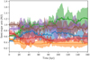 |
Fig. 8 Evolution of the semi-major axis, periapsis, and apoapsis for a typical initial condition. The bold curve is the semi-major axis, and the filled region represents the extent of the orbit. The mutual inclinations are not represented. |
Summary of the main statistics and specifications of the spatial and eccentric runs.
8 Comparison with existing integrators
We ran the same eccentric and inclined initial conditions using the REBOUND (Rein & Liu 2012) package integrators IAS15 (Rein & Spiegel 2015) and MERCURIUS (Rein et al. 2019). IAS15 is an adaptive high-order Gauss-Radau integrator, and MERCURIUS is a hybrid symplectic integrator similar to MERCURY (Chambers 1999). This choice is motivated because the REBOUND team made recent and precise comparisons with other available integrators (Rein & Spiegel 2015; Rein & Tamayo 2015). Moreover, we used a very similar implementation of the Kepler step. We also ran the same tests with the multi-time-step symplectic integrator SYMBA (Duncan et al. 1998).
We plot in Fig. 11 the energy error median that results from the integration. Our integrator performs similarly to the non-symplectic integrator IAS15 and better than MERCURIUS and SYMBA. Our integrator runs at the same speed as MERCURIUS and SYMBA with a time-step of Δt = 10−4. However, IAS15 is much faster on this particular problem (by a factor 10 on average). MERCURIUS and SYMBA are not designed to work efficiently at such low-energy errors. However, our motivation for this work was to find a precise symplectic integrator for close encounters. We thus tried to obtain the best precision from MERCURIUS and SYMBA to make the comparison relevant.
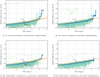 |
Fig. 9 Evolution of the energy error for the four runs detailed in the text and Table 1. The light curves represent individual systems, and the thicker blue curves show the medians over the 100 systems. The orange filled lines are proportional to |

 |
Fig. 10 PDFof the closest approach during close encounters. The PDFs of the four runs are almost identical. |
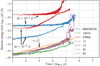 |
Fig. 11 Comparison of the different adaptive integrator runs presented in Table 1 to other codes: IAS15, MERCURIUS, and SYMBA. The same initial conditions were integrated. We plot the median of the energy error. |
9 Discussion
We showed that time renormalisation can lead to very good results for the integration of highly unstable planetary systems using a symplectic integrator (Sect. 3). The algorithm can use a scheme of arbitrary order, however, we have not been able to take advantage of the hierarchical structure beyond the first order in ε. This is due to the non linearity of the time renormalisation as explained in Sect. 4. It is possible, however, to cancel every term up to arbitrary order in the time-step using non-hierarchical schemes.
Our time renormalisation uses the perturbation energy to monitor when two planets encounter each other. The algorithm is thus efficient if the two-planet interaction contributes to a significant part of the perturbation energy. As a result, this integrator is particularly well adapted for systems of a few planets (up to a few tens) with similar masses (within an order of magnitude). Moreover, itbehaves extremely well in the two-planet problem even when one planet mass is significantly lower than the other.
However, the algorithm is not yet able to spot close encounters between terrestrial planets in a system that contains giant planets, such as the solar system. In the case of the solar system, the perturbation energy is dominated by the interaction between Jupiter and Saturn. We plan to address this particular problem in the future.
Appendix A Implementation
We give technical details on our implementation choices in this appendix.
A.1 Kepler equation
The key step in any Wisdom–Holman algorithm is the numerical resolution of the Kepler problem,
 (A.1)
(A.1)
where  and M is the central mass in the set of coordinates used in the integration. Because this is the most expensive step from a computational point of view, it is particularly important to optimise it. Here, we closely followed the works by Mikkola (1997) and Mikkola & Innanen (1999) and refer to them for more details. Rein & Tamayo (2015) presented an unbiased numerical implementation that can be found in the package REBOUND2.
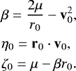
We consider a planet with initial conditions r0 and v0. The goal is to determine the position of the planet r and its velocity v along the Keplerian orbit after a time t. In order to avoid conversions from Cartesian coordinates into elliptical elements, we use the Gauss f- and g-function3 formalism (e.g. Wisdom & Holman 1991). We have
![Mathematical equation: \begin{align*} {\bf{r}}&= f \r_0 + g \v_0,\nonumber\\[2pt] \mathbf{v}& = \dot f \r_0 + \dot g \v_0,\end{align*}](/articles/aa/full_html/2019/08/aa35786-19/aa35786-19-eq117.png) (A.2)
(A.2)
where the values of f, g, ḟ and ġ depend on t, r0, and v0 and are given in Eq. (A.7). When two planets encounter each other, their orbits may become hyperbolic. To be able to resolve these events as well as ejection trajectories, we use a formulation of the Kepler problem that allows hyperbolic orbits. In order to do so, Stumpff (1962) developed a general formalism that contains the hyperbolic and elliptical case in the same equations. Moreover, this approach avoids the singularity for an eccentricity close to 1. Stumpff introduced special functions
 (A.3)
(A.3)
The c-functions allows us to compute the so-called G-functions (Stiefel & Scheifele 1971), which are defined as
 (A.4)
(A.4)
In this formalism, the Kepler equation takes the form (Stumpff 1962)
 (A.5)
(A.5)
of unknown  and where
 (A.6)
(A.6)
In Eq. (A.5), X plays a similar role to the eccentric anomaly in the classical form. Equation (A.5) can be solved by the Newton method (Rein & Tamayo 2015). The new position and velocity are then obtained with Eq. (A.2) and
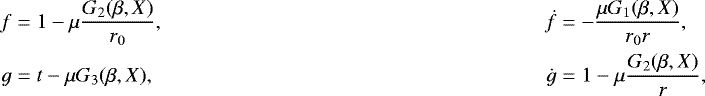 (A.7)
(A.7)
where r = r0 + η0G1 + ζ0G2.
A.2 Computing the effective time-step
In both the Kepler and the perturbation step, it is important to precisely compute the effective time-step (20). For the Kepler step in particular, τ0 depends on the difference H0 − E0, where H0 and E0 are similar. To avoid numerical errors, we compute the initial energy with compensated summation (Kahan 1965). We save the value and the associated error. We then evaluate the Keplerian energy H0 using compensated summation and then derive the difference. Compensated summation is also used to update the positions and velocities, and to integrate the real time equation.
During the numerical tests, we realised that in Jacobi coordinates, the perturbation energy H1 is most of the time lower by almost an order of magnitude than the typical planet energy interaction E1. On the other hand, H1 and E1 are roughly of the same order for heliocentric coordinates. This shows that the algorithm is less efficient in the detection of an increase in interaction energy (that monitors the close encounters). To circumvent this problem, we slightly modify Eq. (20) for Jacobi coordinates. The effective step sizes are computed with
 (A.8)
(A.8)
The total energy sum is still zero,
 (A.9)
(A.9)
which preserves the equation of motion according to Eq. (13). With this modification, the results between Jacobi and heliocentric coordinates are comparable.
Appendix B MacLachlan high-order schemes
In McLachlan (1995a), the scheme coefficients wi are the coefficients for a symmetric composition of second-order steps. We list in Table B.1 the corresponding coefficients ai and bi for the schemes that we used,  and
and  . McLachlan provided 20 significant digits, therefore we made the computation in quadruple precision and truncated to the appropriate precision.
Coefficients of the schemes used in this article.
References
- Blanes, S., & Iserles, A. 2012, Celest. Mech. Dyn. Astron., 114, 297 [NASA ADS] [CrossRef] [Google Scholar]
- Blanes, S., Casas, F., Farrés, A., et al. 2013, Appl. Num. Math., 68, 58 [CrossRef] [Google Scholar]
- Brouwer, D. 1937, AJ, 46, 149 [NASA ADS] [CrossRef] [Google Scholar]
- Chambers, J. E. 1999, MNRAS, 304, 793 [NASA ADS] [CrossRef] [MathSciNet] [Google Scholar]
- Chambers, J., Wetherill, G., & Boss, A. 1996, Icarus, 119, 261 [NASA ADS] [CrossRef] [MathSciNet] [Google Scholar]
- Dehnen, W., & Hernandez, D. M. 2017, MNRAS, 465, 1201 [NASA ADS] [CrossRef] [Google Scholar]
- Duncan, M. J., Levison, H. F., & Lee, M. H. 1998, AJ, 116, 2067 [NASA ADS] [CrossRef] [EDP Sciences] [Google Scholar]
- Farrés, A., Laskar, J., Blanes, S., et al. 2013, Celest. Mech. Dyn. Astron., 116, 141 [NASA ADS] [CrossRef] [Google Scholar]
- Gladman, B., Duncan, M., & Candy, J. 1991, Celest. Mech. Dyn. Astron., 52, 221 [NASA ADS] [CrossRef] [Google Scholar]
- Hairer, E., Lubich, C., & Wanner, G. 2006, Geometric Numerical Integration: Structure-Preserving Algorithms for Ordinary Differential Equations (Berlin: Springer Science & Business Media) [Google Scholar]
- Hernandez, D. M. 2016, MNRAS, 458, 4285 [NASA ADS] [CrossRef] [Google Scholar]
- Hernandez, D. M., & Bertschinger, E. 2015, MNRAS, 452, 1934 [NASA ADS] [CrossRef] [Google Scholar]
- Kahan, W. 1965, Commun. ACM, 8, 40 [CrossRef] [Google Scholar]
- Kinoshita, H., Yoshida, H., & Nakai, H. 1991, Celest. Mech. Dyn. Astron., 50, 59 [NASA ADS] [CrossRef] [Google Scholar]
- Koseleff, P. V. 1993, in Applied Algebra, Algebraic Algorithms and Error-Correcting Codes, eds. G. Cohen, T. Mora, & O. Moreno, Lecture Notes in Computer Science (Berlin: Springer Berlin Heidelberg), 213 [Google Scholar]
- Laskar, J. 1990, in Les Méthodes Modernes de La Mécanique Céleste. Modern Methods in Celestial Mechanics, 89 [Google Scholar]
- Laskar, J., & Gastineau, M. 2009, Nature, 459, 817 [NASA ADS] [CrossRef] [PubMed] [Google Scholar]
- Laskar, J., & Robutel, P. 2001, Celest. Mech. Dyn. Astron., 80, 39 [NASA ADS] [CrossRef] [Google Scholar]
- Laskar, J., Gastineau, M., Delisle, J.-B., Farrés, A., & Fienga, A. 2011, A&A, 532, L4 [NASA ADS] [CrossRef] [EDP Sciences] [Google Scholar]
- Marchal, C., & Bozis, G. 1982, Celest. Mech., 26, 311 [Google Scholar]
- McLachlan, R. 1995a, SIAM J. Sci. Comput., 16, 151 [CrossRef] [MathSciNet] [Google Scholar]
- McLachlan, R. I. 1995b, BIT Num. Math., 35, 258 [CrossRef] [Google Scholar]
- Mikkola, S. 1997, Celest. Mech. Dyn. Astron., 67, 145 [NASA ADS] [CrossRef] [Google Scholar]
- Mikkola, S. 2008, in Dynamical Evolution of Dense Stellar Systems (Cambridge: University Press), 246, 218 [NASA ADS] [Google Scholar]
- Mikkola, S., & Innanen, K. 1999, Celest. Mech. Dyn. Astron., 74, 59 [NASA ADS] [CrossRef] [Google Scholar]
- Mikkola, S., & Tanikawa, K. 1999, Celest. Mech. Dyn. Astron., 74, 287 [NASA ADS] [CrossRef] [Google Scholar]
- Petit, A. C., Laskar, J., & Boué, G. 2018, A&A, 617, A93 [NASA ADS] [CrossRef] [EDP Sciences] [Google Scholar]
- Preto, M., & Tremaine, S. 1999, AJ, 118, 2532 [NASA ADS] [CrossRef] [Google Scholar]
- Rein, H., & Liu, S.-F. 2012, A&A, 537, A128 [NASA ADS] [CrossRef] [EDP Sciences] [Google Scholar]
- Rein, H., & Spiegel, D. S. 2015, MNRAS, 446, 1424 [NASA ADS] [CrossRef] [Google Scholar]
- Rein, H., & Tamayo, D. 2015, MNRAS, 452, 376 [NASA ADS] [CrossRef] [Google Scholar]
- Rein, H., Hernandez, D. M., Tamayo, D., et al. 2019, MNRAS, 485, 5490 [NASA ADS] [CrossRef] [Google Scholar]
- Stiefel, E. L., & Scheifele, G. 1971, Linear and Regular Celestial Mechanics. (Berlin: Springer) [CrossRef] [Google Scholar]
- Stumpff, K. 1962, Himmelsmechanik, Band I (Berlin: VEB Deutscher Verlag der Wissenschaften) [Google Scholar]
- Wisdom, J. 2006, AJ, 131, 2294 [NASA ADS] [CrossRef] [MathSciNet] [Google Scholar]
- Wisdom, J., & Holman, M. 1991, AJ, 102, 1528 [NASA ADS] [CrossRef] [Google Scholar]
- Wisdom, J., Holman, M., & Touma, J. 1996, Fields Inst. Commun., 10, 217 [Google Scholar]
- Yoshida, H. 1990, Phys. Lett. A, 150, 262 [Google Scholar]
We use the convention  .
.
These functions are different from the time-renormalisation functions used in this article.
All Tables
Summary of the main statistics and specifications of the spatial and eccentric runs.
All Figures
|
Fig. 1 Upper panel: f ′, Eq. (22) as a function of h∕E1. The asymptotic value for h∕E1 → +∞ is given in green. Lower panel: f∕E1, Eq. (23) as a function of h∕E1. |
| In the text | |
|
Fig. 2 Comparison between various schemes detailed in the body of the text for the integration of a single synodic period for a system of equal-mass planets initially on planar circular orbits with ε = 2m∕m0 = 10−5 and α = 0.8. The solid lines represent the integrations using a fixed real time-step and the dots the adaptive time-steps. The closest planet approach is 0.19992 AU. |
| In the text | |
|
Fig. 3 Same as Fig. 2 for a system of two equal-mass planets initially on planar circular orbits with ε = 2m∕m0 = 10−5 and α = 0.97. The closest planet approach is 3.68 × 10⁻⁵ AU. |
| In the text | |
|
Fig. 4 Same as Fig. 2 for a system of two equal-mass planets initially on planar circular orbits with ε = 2 m∕m0 = 10−3 and α = 0.9. The closest planet approach is 1.7 × 10⁻² AU. This systemis integrated in heliocentric coordinates to demonstrate that we obtain similar results to the case of Jacobi coordinates. |
| In the text | |
|
Fig. 5 Mutual distance of the planets as a function of the fictitious time for 1000 initial conditions chosen as described in the body of the text. On the upper axis, we give the real time for the initial condition that reached the closest approach. |
| In the text | |
|
Fig. 6 Relative energy error as a function of the closest mutual approach reached during a close encounter of super-Earths in a two-planet system and in a six-planet system. The particular initial conditions are described in the text. In the upper part, we give the mutual distance in units of planet radii for a planet of density ρ = 6 g cm−3. |
| In the text | |
|
Fig. 7 Evolution of the relative energy error for 100 systems composed of six planets on initially circular orbits. The light curves represent individual systems, and the thicker blue curves show the average over the 100 systems. The orange straight line is proportional to
|
| In the text | |
|
Fig. 8 Evolution of the semi-major axis, periapsis, and apoapsis for a typical initial condition. The bold curve is the semi-major axis, and the filled region represents the extent of the orbit. The mutual inclinations are not represented. |
| In the text | |
|
Fig. 9 Evolution of the energy error for the four runs detailed in the text and Table 1. The light curves represent individual systems, and the thicker blue curves show the medians over the 100 systems. The orange filled lines are proportional to |
| In the text | |
|
Fig. 10 PDFof the closest approach during close encounters. The PDFs of the four runs are almost identical. |
| In the text | |
|
Fig. 11 Comparison of the different adaptive integrator runs presented in Table 1 to other codes: IAS15, MERCURIUS, and SYMBA. The same initial conditions were integrated. We plot the median of the energy error. |
| In the text | |
Current usage metrics show cumulative count of Article Views (full-text article views including HTML views, PDF and ePub downloads, according to the available data) and Abstracts Views on Vision4Press platform.
Data correspond to usage on the plateform after 2015. The current usage metrics is available 48-96 hours after online publication and is updated daily on week days.
Initial download of the metrics may take a while.