| Issue |
A&A
Volume 697, May 2025
|
|
|---|---|---|
| Article Number | A101 | |
| Number of page(s) | 10 | |
| Section | Stellar structure and evolution | |
| DOI | https://doi.org/10.1051/0004-6361/202452899 | |
| Published online | 12 May 2025 | |
X-ray and radio data obtained by XMM-Newton and VLA constrain the stellar wind of the magnetic quasi-Wolf-Rayet star in HD45166
1
Osservatorio Astrofisico di Catania, INAF, Via S. Sofia 78, I-95123 Catania, Italy
2
Institute for Physics and Astronomy, University Potsdam, Karl-Liebknecht-Str. 24/25, D-14476 Potsdam, Germany
3
The School of Physics and Astronomy, Tel Aviv University, 6997801 Tel Aviv, Israel
4
Department of Physics and Space Science, Royal Military College of Canada, PO Box 17000, Kingston, ON K7K 7B4, Canada
5
Department of Physics and Astronomy, University of Delaware, 217 Sharp Lab, Newark, DE 19716, USA
6
Department of Physics & Astronomy, East Tennessee State University, 173 Sherrod Drive, Johnson City, TN 37614, USA
7
Penn State Scranton, Pennsylvania State University, 120 Ridge View Drive, Dunmore, PA 18512, USA
⋆ Corresponding authors: This email address is being protected from spambots. You need JavaScript enabled to view it.
; This email address is being protected from spambots. You need JavaScript enabled to view it.
Received:
6
November
2024
Accepted:
22
March
2025
Abstract
Context. Recently, a powerful magnetic field was discovered in the hot helium star classified as a quasi-Wolf-Rayet (qWR) star (∼2 M⊙), in the HD 45166 system. Upon its explosion as a core-collapse supernova, it is expected to produce a strongly magnetic neutron star – a magnetar. Among the key parameters that govern pre-supernova evolution is the amount of mass lost via stellar wind. However, the magnetic nature of this helium star is expected to affect its stellar wind, which makes the estimation of the wind parameters uncertain.
Aims. We report the first observations of HD 45166 in X-rays with the XMM-Newton telescope and in radio with the VLA interferometer array. By placing the observation results in a theoretical framework, we aim to provide a reliable estimate of the wind strength of the magnetic qWR star.
Methods. We explain the X-ray properties in the framework of the magnetically confined wind shock scenario, and we apply the semianalytic model of a dynamical magnetosphere (DM) to reproduce the X-ray emission. We compute the thermal radio emission of the wind and its absorption effect on possible gyro-synchrotron emission from the underlying dipolar magnetosphere, sampled in 3D, by integrating the radiative transfer equation.
Results. We did not detect radio emissions, which enabled us to set sensitive upper limits on the radio luminosity. The magnetic qWR star is a slow rotator, and comparison with models reveals that the possible acceleration mechanisms that occur within its DM are not as efficient as in fast-rotating magnetic ApBp-type stars. In contrast, the system is detected in X-rays with log(LX/Lbol)∼−5.6. Using suitable models, we constrain the mass lost from this magnetic quasi-Wolf-Rayet star as Ṁ ≈ 3 × 10⁻¹⁰ M⊙ yr−1.
Conclusions. This novel empirical estimate of the mass-loss rate in a ∼2 M⊙ helium star confirms that it maintains super-Chandrasekhar mass until collapse and can produce a magnetar as its final evolutionary product.
Key words: radiation mechanisms: non-thermal / radiation mechanisms: thermal / stars: magnetars / stars: mass-loss / stars: winds, outflows / stars: Wolf-Rayet
© The Authors 2025
 Open Access article, published by EDP Sciences, under the terms of the Creative Commons Attribution License (https://creativecommons.org/licenses/by/4.0), which permits unrestricted use, distribution, and reproduction in any medium, provided the original work is properly cited.
This article is published in open access under the Subscribe to Open model. This email address is being protected from spambots. You need JavaScript enabled to view it. to support open access publication.
1. Introduction
The binary system HD 45166 consists of a hot helium star and a B7 V-type star (Willis & Stickland 1983) bound with an orbital period of 22 yr (Shenar et al. 2023). The optical spectrum of the helium star is dominated by emission lines of carbon, nitrogen, and oxygen in high ionization states, hence warranting its Wolf-Rayet (WR) spectral classification (Anger 1933; Neubauer & Aller 1948; Hiltner & Schild 1966). The relatively low luminosity of the helium star compared to classical WR stars, in combination with its uniquely narrow emission lines and unusual abundance pattern, gave rise to its designation as a quasi-Wolf-Rayet (qWR) star (van Blerkom 1978). The mass of the qWR star was originally estimated at 0.5 M⊙ (Willis & Stickland 1983), then raised to ≈4 M⊙ (Groh et al. 2008), and finally revised as M* = 2.03±0.44 M⊙ (Shenar et al. 2023). While this mass is at the lower limit needed for core collapse (Woosley et al. 1995), the final fate of the qWR component is uncertain, and whether or not the star will produce a supernova (SN) will depend on the amount of mass it loses until core collapse.
The characteristics of the helium star in HD 45166 make it a prototype for super-Chandrasekhar mass stars stripped of their outer hydrogen layers. Helium stars of such masses are generally thought to form via interactions among components in close binaries (Podsiadlowski et al. 1992; Yungelson et al. 2024). This evolutionary channel can lead to the formation of helium-rich stars that are significantly less massive than the classical WR stars (i.e., ≲10 M⊙; Hamann et al. 2019; Sander et al. 2019; Shenar et al. 2020). Binary evolution models predict that stripped stars are hot and numerous; as such, they could be among the dominant ionizing sources in star-forming galaxies and may represent the bulk of progenitors of stripped supernovae (Dionne & Robert 2006; Götberg et al. 2018; Doughty & Finlator 2021). Finding super-Chandrasekhar-mass helium stars stripped by binary interactions has proved difficult (Ramachandran et al. 2023; Drout et al. 2023; Gilkis & Shenar 2023), and for a long time the qWR star in the HD 45166 system was the only well-studied candidate.
Of special interest is the mass-loss rate of these objects, which determines the properties of the pre-collapse core. Radiation fields of hot, OB-, and WR-type stars drive stellar winds (Castor et al. 1975). Previous analyses of the optical spectrum of the qWR star by means of latitude-dependent wind models derived a mass-loss rate of Ṁ ≈ 2 × 10⁻⁷ M⊙ yr−1 (with an equatorial wind velocity of  km s−1 and a polar terminal wind velocity of
  km s−1; Willis & Stickland 1983; Willis et al. 1989; Groh et al. 2008). These values are significantly different from the theoretical predictions. Vink (2017) explored the parameter space that characterizes winds from helium stars. The mass of the helium star (or equivalently its luminosity given the mass-luminosity relation) has been varied in the range from 60 M⊙ to 0.6 solar masses, with a fine tuning in the range 2–20 M⊙. Once assigned metallicity and mass, the Monte Carlo modeling approach performed by Vink (2017) provides both the mass-loss rate and the terminal wind velocity. In particular, the mass-loss rate predicted for a 2 M⊙ star at Solar metallicity is Ṁth ≈ 4 × 10⁻⁹ M⊙ yr−1, while the predicted wind velocity is
  km s−1.
The striking difference between the empirically measured mass-loss rate and wind velocity of the qWR star and the theoretical predictions has already been noticed by Vink (2017). However, the recent discovery of a strong magnetic field on the qWR star suggests that its wind is strongly affected by magnetic field and calls for new approaches in evaluating its stellar wind parameters. In this paper, we address this problem using new X-ray and radio observations.
The qWR possesses an exceptionally strong magnetic field of 〈B〉∼43 kG. This breaks the record held by Babcock's Star (∼34 kG; Babcock 1960) making the qWR the most strongly magnetic non-degenerate star known. The qWR is likely to be a merger product in an initially triple system, with the non-magnetic B7 V component being an original tertiary, and it is predicted to end its life as a strongly magnetic neutron star: a magnetar (Shenar et al. 2023).
The high magnetic field of the qWR star plays a major role in regulating its mass loss. The magnetic field affects the free radial flow of the stellar wind up to a certain distance, named Alfvén radius (RA), which leads to a so-called confined wind structure. Hence, the spectrum of the qWR star forms in its magnetosphere, which must be taken into account in empirical mass-loss rate measurements.
The magnetic star in the HD 45166 system is a very slow rotator; its rotation period exceeds 100 days (Table 1). This is a suitable condition for originating a dynamical magnetosphere (DM), which commonly characterizes the slowly rotating massive magnetic stars that have a radiatively driven stellar wind (Petit et al. 2013). Furthermore, the combined presence of wind and magnetic field allows us to place the qWR in the context of other hot massive magnetic stars such as ApBp-type stars that are, in general, X-ray and radio sources (Drake et al. 1987, 1994; Linsky et al. 1992; Leone et al. 1994; Oskinova et al. 2011; Nazé et al. 2014). Production of X-rays in magnetic hot stars is usually explained by the cooling of a fraction of their stellar winds, which are heated to a few million degrees by strong shocks that result from the collision of streams confined by a magnetic field (magnetically confined wind shock, MCWS, model; Babel & Montmerle 1997; ud-Doula & Nazé 2016). This helps to explain why some magnetic stars are more X-ray luminous compared to their non-magnetic counterparts (Oskinova et al. 2011; Nazé et al. 2014).
Parameters of the magnetic qWR star in the HD 45166 system.
Magnetohydrodynamic (MHD) simulations predict that the continuous supply of wind material to the magnetospheres in slowly rotating stars is balanced by the plasma infall back onto the stellar surface (ud-Doula & Owocki 2002; ud-Doula et al. 2008, 2013). Beyond the Alfvén radius, the breaking of the magnetic field lines should lead to particle acceleration (Usov & Melrose 1992). Fast non-thermal electrons power both incoherent non-thermal gyro-synchrotron and coherent auroral radio emission (Trigilio et al. 2000; Das et al. 2022) and, in some cases, also non-thermal X-rays of auroral origin (Leto et al. 2017; Robrade et al. 2018).
Thus, radio and X-ray observations are excellent probes of conditions in stellar magnetospheres. To gain insight into the wind properties of the qWR star and its magnetosphere, we obtained new observations in the X-ray and radio domains. In Sect. 2 we describe the observations and data reduction. In Sect. 3 we report the observational results directly derived from the analysis of the X-ray (Sect. 3.1) and radio (Sect. 3.2). In Sect. 4.1 we provide the theoretically expected X-ray spectrum; in Sect. 4.2 we describe how the stellar wind is affected by its strong magnetic field. The physical mechanisms that affect the radio emission are explored in Sect. 5; in Sect. 5.1 we discuss the possible non-thermal electron production and, after taking into account the frequency-dependent absorption effect due to the large-scale distributed wind plasma, the upper limit of the corresponding non-thermal radio emission is calculated in Sect. 5.2. Finally, in Sect. 5.3 we place our results in a general framework that includes O-type magnetic stars. In Sect. 6 we present our conclusions and discuss how the forthcoming sensitive radio facilities may be useful for the science case discussed in this paper.
2. Observations and data reduction
2.1. Radio
The radio observations were performed at the Very Large Array (VLA) National Radio Astronomy Observatory in November 2022; the observing log is reported in Table 2. The observations were conducted in three bands: the C-band, centered at ν = 5.5 GHz; the X-band, centered at ν = 9 GHz; and the Ku-band, centered at ν = 15 GHz. For the C and X bands, the adopted hardware setup allowed us to observe a bandwidth of 2 GHz width (8-bit digital samplers), whereas the adopted setup for the Ku-band observations allowed us to recover flux within a wider spectral range, at a bandpass of 6 GHz using the 3-bit digital samplers.
Log of the VLA Observations of HD 45166. Array Config C. Code: 22B-314.
To calibrate the flux scale and the receiver's response within the spectral range covered by the VLA receivers (bandpass calibration), the radio galaxy 3C286 (1331+305) was observed as the primary calibrator in each observing band. To calibrate the amplitude and phase of the complex gain, the standard VLA calibrator J0613+1306 was cyclically observed for each band during the observing scans. J0613+1306 is a point-like radio source located close to the sky position of HD 45166 (about 6° away) with an almost flat radio emission level (≈0.5 Jy) in the range 5–15 GHz. The observations were processed through the VLA Calibration Pipeline (version 2022.2.0.64), which is designed to handle Stokes I continuum data, operating within the Common Astronomy Software Applications (CASA) package (release 6.4.1). Images of the sky region centered at the target position were obtained using the task TCLEAN (number of Taylor terms 2, number of clean iterations 40 000).
HD 45166 is located in a sky region not contaminated by strong radio sources and the radio maps of the total intensity (Stokes I) show no issues. In fact, we measured low noise levels in each band (RMS<8 μJy/beam, see Table 2), which nearly coincide with the levels expected in each band, as confirmed by the VLA exposure calculator1 once the same parameters of the observations were set (bandwidth and times on the source), which confirms the goodness of the VLA observations. Despite the high-quality radio measurements, HD 45166 is not detected.
2.2. X-rays
X-ray data were acquired with the X-Ray Multi-Mirror Mission (XMM-Newton) of the European Space Agency (ESA). XMM-Newton has three X-ray telescopes that illuminate five different instruments, which always operate simultaneously and independently. The useful data were obtained with the three focal instruments: MOS1, MOS2, and pn, which together form the European Photon Imaging Camera (EPIC). The EPIC instruments have a broad wavelength coverage of 1.2–60 Å and allow for low-resolution spectroscopy with (E/ΔE≈20−50). Throughout this paper, X-ray fluxes and luminosities are given for the full energy band.
The XMM-Newton observations of HD 45166 were carried out on 2022 Sep. 11 with a total duration ∼20 ks (ObsID 0900520101). All three EPIC cameras were operated in the standard, full-frame mode. The “medium” UV filter was used for MOS cameras, while the “thin” filter was used for the pn. The observations were affected by episodes of high background. After rejecting these time intervals, the cumulative useful exposure time was ≈6 ks for the EPIC pn and ≈12 ks for the EPIC MOS cameras. No significant source variability is seen during these exposure times. The data were analyzed using the XMM-Newton data analysis package SAS2. The customary and the pipeline-reduced data are consistent.
Contrary to the radio, HD 45166 is clearly detected in all XMM-Newton cameras. The total EPIC count rate from the isolated X-ray source at the position of HD 45166 is 0.23±0.01 s−1. The X-ray spectra and light curves of HD 45166 were extracted using standard procedures from a region with a radius of ≈20″. The background area was chosen to be nearby the star and free of X-ray sources. There are ≈1100 spectral data counts registered by the pn camera, while the MOS cameras registered ≈1040 spectral counts.
To analyze the X-ray spectra of HD 45166, we used the standard spectral fitting software XSPEC (Arnaud 1996). The abundances were set to the HD 45166 abundances (Shenar et al. 2023) using the method outlined in Oskinova et al. (2012, 2020). In all spectral models, the absorption in the interstellar medium is included using the TBABS model (Wilms et al. 2000). The distance and reddening of HD 45166 are reported in Table 1.
3. Results
3.1. X-ray diagnostic of the hot plasma
The HD 45166 system contains a non-magnetic B7 V-type star. Late B-type non-magnetic stars do not emit X-rays (Stelzer et al. 2005; Evans et al. 2011), therefore we attribute all X-rays detected in HD 45166 to its helium star companion only.
X-ray spectra of HD 45166 are shown in the top panel of Fig. 1. The corresponding unbinned EPIC pn spectrum of HD 45166 is shown in the bottom panel of Fig. 1, where a prominent emission line at λ≈1.87 Å is clearly seen. This line belongs to the He-like Fe XXV ion, which has a peak emissivity at kT = 5.4 keV (T≈60 MK).
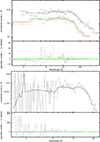 |
Fig. 1. Top panel: XMM-Newton pn (upper black crosses), and MOS1 and MOS2 (lower green and red crosses) spectra of HD 45166 where a suitable number of instrumental channels are binned, but not more than 300, to achieve at least a 3σ detection. Bottom panel: XMM-Newton unbinned EPIC pn spectra corrected for the instrument response (black crosses) of HD 45166, with error bars corresponding to 1σ. The best-fit model is a combination of three thermal VAPEC models. |
To determine the physical conditions of the plasma, we fitted the observed spectra using the Astrophysical Plasma Emission Code “apec” (Smith et al. 2001), which is a state-of-the-art code able to model a thermal optically thin plasma in collisional equilibrium. We used the VAPEC version of the code that allows for non-solar abundances. The simulated spectrum superimposed to the observed one (binned and unbinned) is pictured in Fig. 1.The corresponding model parameters are shown in Table 3. When we apply the relation NH, ISM=EB−V·6.12×1021 cm−2 (Gudennavar et al. 2012), the interstellar column density is (1.28±0.06)×1021 cm−2. This is consistent with the NH values inferred from the adopted X-ray model (see Table 3). When we adopt the distance and the reddening from Table 1, the X-ray luminosity of HD 45166 (Table 3) is log(LX [erg s−1])≈31.8, which corresponds to a ratio between X-ray and bolometric luminosity of log(LX/Lbol)≈−5.6, that is among the highest ratios of known OB and WR-type stars without a compact binary companion (Nazé et al. 2014; Nebot Gómez-Morán & Oskinova 2018).
X-ray spectral parameters.
The combination of three temperature components is sufficient to fit the low-resolution X-ray spectrum of HD 45166. The individual model components are shown in Fig. 2. The lower temperature plasma components have T≈6 and 13 MK, whereas the highest temperature plasma has T≈70 MK (kT≈5.7 keV), the largest emission measure (EM) among the three plasma components (Table 3), and it is also responsible for the short wavelengths (λ<2 Å) emission lines. To explain this high temperature by the Rankine-Hugoniot shock condition, where the temperature of the plasma after the shock is related to the pre-shock velocity as  , where V3=V/(103 km s−1), a velocity jump of about 2200 km s−1 is required. Therefore, if X-rays originate from shocks that occur in the magnetically confined wind, the three thermal components could be the tracers of the temperature range of the regions where the shocks dissipate energy.
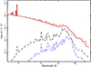 |
Fig. 2. Contributions from individual three temperature thermal components to the best-fit spectral model. The three lines (dashed-dotted blue, dashed black, dotted black) show the spectral models that correspond to individual components (see Table 3). The solid red line shows the best-fit combined model. |
3.2. Radio diagnostic of the stellar wind
Any ionized stellar wind also emits thermal radio. For a spherical non-magnetic wind, the radio spectrum is described by Sν ∝ Ṁ4/3ν0.6 (Wright & Barlow 1975; Panagia & Felli 1975), with the radio flux then providing a measure of the mass-loss rate. The full expression for calculating the theoretical spectrum of thermal radio emission from a stellar wind is given by Scuderi et al. (1998):
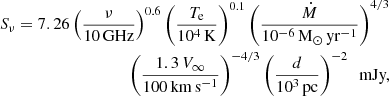 (1)
(1)
where the wind temperature (Te) is assumed to be 85% of the effective stellar temperature.
No radio emission is detected at the position of HD 45166 and only upper limits on the flux in three radio bands could be determined. We can use the stringent upper limits on the fluxes in three radio bands (lying in the range 15–24 μJy, which is the 3σ detection threshold estimated by the map noises listed in Table 2) to constrain the mass-loss rate of the stellar wind by Eq. (1).
In the absence of a strong globally organized magnetic field, the mass-loss rate, Ṁ(B = 0), could be theoretically predicted and empirically measured by conventional spectroscopic methods. The strong, likely dipolar, magnetic field of the qWR star should strongly alter the topology of its stellar wind. While at low magnetic latitudes the wind is trapped, it is free to escape from the magnetic polar regions. It is reasonable to expect that the radial component of the polar wind is larger compared to the wind at low magnetic latitudes, which is trapped by the magnetic field and forced to flow along the magnetic field lines, thus the wind speed has no radial component near the magnetic equator. This may explain the differences between the wind terminal velocities at the equator and the pole ( km s−1 and
  km s−1; Groh et al. 2008).
The wind of the qWR star is expected to be confined by the dipole magnetic field up to the Alfvén radius, and only beyond it the ionized material can escape like a nearly spherical non-magnetic wind. At a large distance, the stellar wind that emerges from the polar regions fills a major fraction of the spherical volume. Therefore, the upper limit on radio emission allows us to establish an upper limit on the mass-loss rate of the escaping wind. The strongest constraint for the mass-loss rate of the freely escaping wind is given by the observation in the 15 GHz band, which has the highest sensitivity (see Table 2) and corresponds to a 3σ detection threshold of 15 μJy. We calculated radio spectra using Eq. (1) and only varied the parameter Ṁ, while the terminal velocity was fixed to  km s−1.
The maximum mass-loss rate of the qWR star that produces thermal radio emission with an emission level that does not contradict the VLA non-detection is Ṁmax = 1.1 × 10⁻⁷ M⊙ yr−1, which is about a factor of two lower than the mass-loss rate of 2.2×10⁻⁷ M⊙ yr−1 found by Groh et al. (2008). The corresponding theoretical wind spectrum is pictured in Fig. 3 (solid black line). If we assume as a check the equatorial wind velocity, that is  km s−1, a mass-loss rate of about 3.9×10⁻⁸ M⊙ yr−1, which is lower than Ṁmax, is required to be consistent with the upper limits in radio. Therefore, our radio observations definitively rule out the wind parameter combination that corresponds to the lower value of the terminal wind velocity, V∞ = 425 km s−1, and the mass-loss rate of 2.2×10⁻⁷ M⊙ yr−1 (Groh et al. 2008) as global properties of the wind escaping from the qWR star.
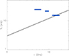 |
Fig. 3. Theoretical wind spectrum constrained by the detection thresholds. The blue boxes correspond to the 3σ noise levels measured at the sky position of HD 45166 in radio maps obtained at the three observed bands, which provide the detection threshold. The lengths of the blue boxes show the bandpass for the receivers (see Table 2). The solid black line displays the theoretical thermal wind's spectrum that corresponds to the maximum emission level that is compatible with non-detection below the 3σ threshold (Ṁmax = 1.1 × 10⁻⁷ M⊙ yr−1). |
4. X-rays from the wind of the highly magnetized helium star in the HD 45166 system
4.1. Thermal X-ray emission from the magnetic qWR
To quantify the X-rays emitted by the plasma heated in the framework of the MCWS model, ud-Doula et al. (2014) performed time-dependent MHD simulations that included a full energy equation with radiative cooling. Their analysis of how the associated X-ray emission in dynamical magnetospheres is controlled by a cooling-regulated “shock retreat” led to a semianalytic “XADM” formalism. Once assigned the luminosity, mass, and radius of the star, the XADM model allows us to predict the level and hardness of the intrinsic emitted X-rays as a function of the polar strength of the dipole field, Bp, the mass-loss rate, Ṁ(B = 0), and the terminal speed, V∞, of the stellar wind expected in the absence of magnetic field. The agreement with observations is reached by scaling the predicted X-ray luminosity by an order of magnitude (Nazé et al. 2014). The 10% empirical reduction of the XADM prediction is to account for the lower X-ray emission expected from the dynamic infall of the trapped material, which is not considered in the idealized XADM model. In the following, we scale down the XADM predictions by an order of magnitude.
We modify the XADM formalism to account for the highly unusual properties of the qWR star in HD 45166. For simplicity, we assume a pure helium wind. Furthermore, the polar field strength is assumed to be equal to the average field (〈B〉 = 43 kG). Usually, the polar strength is expected to be higher than the average, but the particular geometry of the qWR (i.e., the dipole is seen pole-on) makes this approximation reasonable.
Using the stellar radius and bolometric luminosity reported in Table 1, the left panel of Fig. 4 shows the contour of the predicted log(LX/Lbol) (above 0.3 keV) set to the luminosity derived from the X-ray observations (log(LX, obs/Lbol) = −5.6; Table 3) as a function of the non-magnetized wind mass-loss rate and terminal speed. The horizontal dashed blue and red lines mark, respectively, the limits of the range of the terminal speed values explored. For convenience, the lower limit ( ) has been fixed at 1200 km s−1, which is the empirical wind speed value (Willis et al. 1989), and the upper limit (
 ) at 2650 km s−1, which is the value predicted by Vink (2017) for a 2 M⊙ helium star without a magnetic field. The corresponding vertical dashed lines mark the associated mass-loss rates, Ṁ(B = 0) = 0.5 × 10⁻⁸ M⊙ yr−1 and 2.3×10⁻⁸ M⊙ yr−1.
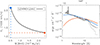 |
Fig. 4. Left: Diagram of the wind parameters of a non-magnetized star; terminal velocity vs. mass-loss rate (the two wind parameters are the free parameters of the XADM model). The black curve represents the loci of the Ṁ(B = 0) and V∞ combination where the XADM model predicts X-ray luminosity coinciding with that empirically determined for the qWR star (Table 3). The horizontal dashed red and blue lines mark, respectively, the lower and upper limits of the range of terminal wind speed values analyzed, with Ṁ(B = 0) tuned to match the observed X-ray luminosity along the black contour (log(LX/Lbol) = −5.6). Right: Associated model X-ray spectra for the fast (solid blue line) and the slower wind model (solid red line). For comparison, the X-ray spectrum of HD 45166 provided by the 3T model without the ISM absorption effect is also displayed (solid black line), the gray solid line is the X-ray spectrum with absorption shown in the left panel of Fig. 2. |
The right panel of Fig. 4 compares the model X-ray spectra that correspond to the velocities extrema, slow (red) and fast (blue). The XADM model with the fast wind has a hard X-ray component not predicted by the model with slower wind, which also has a steeper overall decline at longer wavelengths. A qualitative comparison between the XADM synthetic spectra with the best-fit X-ray spectrum, provided by the pure thermal model once the ISM absorption effect is removed, demonstrates that the X-ray spectral behavior of HD 45166 is closer to the XADM fast wind model, which also suggests that the terminal wind speed could be higher than the fixed upper limit.
Thus the XADM modeling provides an estimate of the combination of wind parameters (mass-loss rate and terminal wind speed) by comparing the shapes of the simulated and observed X-ray spectra. Our analysis showed that a wind with parameters close to those theoretically predicted for a non-magnetic naked helium star with two solar masses (Ṁth ≈ 0.4 × 10⁻⁸ M⊙ yr−1 and  km s−1; Vink 2017) is consistent with the X-ray observations.
4.2. Constraints on the wind parameters of the magnetic qWR
In plasma theory, the ratio between the gas pressure and the magnetic pressure of a stationary plasma defines the parameter β. In the case of a supersonic stellar wind channeled by a dipolar magnetic field, the thermal pressure is replaced by the ram pressure of the wind (Altschuler & Newkirk 1969). Then, the reciprocal of plasma β is
 (2)
(2)
which is the magnetic confinement parameter that characterizes the capability of the stellar magnetic field to channel the wind, which starts on the stellar surface as a radial wind, that is, as a simple non-magnetic spherical wind (ud-Doula & Owocki 2002). In this description, the Alfvén radius is given by the relation (ud-Doula et al. 2008)
 (3)
(3)
If we assume a simple dipole magnetic field, the wind emerging from the stellar surface (Ṁ(B = 0)) could actually only leave the magnetosphere from the magnetic polar caps. The polar caps are delimited by the northern and southern polar rings located by the magnetic latitude of the footprints of the last closed magnetic field line, which is the line that crosses the magnetic equatorial plane at a distance equal to Rc≈1+0.7(RA−1) stellar radii. Following ud-Doula et al. (2008), the wind material lost from a magnetic star can be estimated using the scaling relation
 (4)
(4)
With a polar magnetic field strength equal to 43 kG, the associated magnetic confinement parameter, calculated using Eq. (2) (V∞ = 2650 km s−1 and Ṁ(B = 0) = 0.5 × 10⁻⁸ M⊙ yr−1), is η* = 20 500. The corresponding Alfvén radius calculated using Eq. (3) is RA/R* = 12.3.
In summary, the wind of the qWR star is expected to be confined by the closed dipole magnetic field lines up to the Alfvén radius, and only beyond this radius can the ionized material escape like a nearly spherical non-magnetic wind. The fraction of the wind mass that escapes can be estimated using Eq. (4), that is, about 6% of the wind emerging from the whole stellar surface. The corresponding actual mass-loss rate is ≈3×10⁻¹⁰ M⊙ yr−1, which is about three orders of magnitudes lower than the upper limit constrained by the radio observations (Sect. 3.2), with a related thermal radio emission level of ≈5×10⁻³ μJy (calculated using Eq. (1)).
The wind topology of the qWR is strongly affected by the strong magnetic field. Only a fraction of the fast wind ( km s−1) can escape from the magnetosphere at high magnetic latitudes, and becomes nearly spherical far from the star. Due to the larger area covered by the freely expanding spherical wind, according to the principle of mass continuity, the non-magnetic spherical wind is expected to expand outside the Alfvén surface at a slower velocity with respect to the fast wind velocity required to reproduce the X-ray spectrum of the qWR star. Therefore, the velocity measured in the UV spectrum (V∞(obs.) = 1200 km s−1) is considered as an empirical estimate of the terminal wind velocity of the large-scale spherical wind material actually lost from the qWR star. Figure 5 shows a cartoon that visualizes the scenario described above.
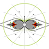 |
Fig. 5. Meridional cross section of the dipole-dominated magnetosphere of HD 45166 (not to scale). At distances smaller than the Alfvén radius (RA), the magnetic field lines are closed. The last closed field lines (marked by the thick solid black line) locates the RA. At larger distances, the ionized wind opens the magnetic field lines. The region where the magnetic field traps the stellar wind is shaded. Outside of the Alfvén surface, the stellar wind freely escapes (black arrows). At lower latitudes, the fast wind plasma streams that arise from opposite hemispheres (thick black arrows) collide and shock. According to the XADM model, the shock heats the plasma producing X-rays (red regions). The equatorial magneto-disk farther than RA (thick black areas) is likely to be the site of the acceleration of electrons (green solid arrows) via magnetic reconnections. Such non-thermal electron population moving within a magnetic shell (delimited by the black and thick solid lines) radiates at the radio regime via the gyro-synchrotron emission mechanism. The outer boundary where the non-thermal electrons diffuse is shown by the solid black open field line. The relativistic electrons radiate in radio bands via a non-thermal emission mechanism (green-shaded regions). The large green circle outlines the optically thick radio photosphere of the freely escaping ionized wind. |
5. Lack of detection of non-thermal radio emission from the qWR in HD 45166
The qWR star is strongly magnetized, and the combined presence of ionized material (wind plasma trapped by the closed magnetic field lines) and a strong magnetic field could provide suitable conditions for non-thermal radio emission powered by the gyro-synchrotron mechanism. In the following, we use the detection threshold obtained by the VLA observations to constrain the plasma parameters that regulate a non-thermal radio emission that is compatible with the non-detection of radio emission from HD 45166.
5.1. Non-thermal electron production within the magnetosphere of the qWR
To better understand the properties of the qWR star, we first consider the case of magnetic ApBp-stars. These are also hot stars with radiatively driven stellar winds confined by strong magnetic fields. Therefore, ApBp-stars provide a useful physical analogy to the “one of its kind” magnetic helium star in HD 45166. Magnetic ApBp-stars have magnetospheres filled by plasma that radiates X-rays; furthermore, these magnetic stars are well-studied non-thermal radio sources. The well-ordered and stable magnetospheres of fast-rotating ApBp stars share a common physical mechanism for supporting the generation of non-thermal electrons, which explains their observational features ranging from the X-ray to radio regime. A general scaling relationship for non-thermal radio emission holds from stars at the top of the main sequence down to ultra-cool dwarfs and to the planet Jupiter (Leto et al. 2021). This is empirically confirmed for ApBp stars (Shultz et al. 2022). The underlying physical process could be related to the breakout events that are predicted in the centrifugally supported magnetospheres (CM) of fast-rotating stars (Owocki et al. 2022). In this case, the radio luminosity is directly related to the power released by the centrifugal breakout events (CBO). In particular, the relation between the spectral radio luminosity and the power of the centrifugal breakouts (LCBO) is Lν, rad = 10−19LCBO Hz−1 (Leto et al. 2022), where
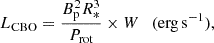 (5)
(5)
and  is the dimensionless critical rotation parameter, defined by the ratio between equatorial velocity and orbital velocity, with G being the gravitational constant.
Using the stellar parameters reported in Table 1, it follows that W≈5.4×10⁻⁴ for the qWR star. Equation (5) predicts the spectral radio luminosity Lν, rad≈2.1×10¹² erg s−1 Hz−1, corresponding to the flux of ≈1.8×10⁻³ μJy, which, in the frequency range covered by the VLA observations, is lower than the expected flux level of the thermal radio emission constrained in Sect. 4. Hence, the CBOs are inefficient as a mechanism for the acceleration of electrons in the magnetic qWR star. This is not surprising since the key condition for the generation of CMs is the Kepler corotation radius (RK), which is smaller than the Alfvén radius. The Kepler radius is given by RK=W−2/3R* (Petit et al. 2013). We estimate RK≈150 R*, which is about an order of magnitude larger than the Alfvén radius estimated in Sect. 4.2 (Table 4); this implies that the qWR does not support a centrifugal magnetosphere.
Magnetospheric parameters of the qWR star.
Let us consider whether stellar wind might play a role in particle acceleration. The wind strength in the qWR star is much higher compared to ApBp-type stars (Oskinova et al. 2011; Krtička et al. 2019), and can break the magnetic field lines relatively close to the star (RA≈12 R*) where the local magnetic field is high enough to trigger plasma effects responsible for non-thermal radio emission (Andre et al. 1988). At distances larger than RA, the magnetic field no longer constraints the wind. The equatorial regions just outside the Alfvén surface are transition regions from the magnetic-dominated to the wind-dominated zones, where the closed dipole-like magnetic field configuration becomes open. These are likely sites of large-scale magnetic field reorganization, with the consequent formation of a magneto-disk, which possibly gives rise to current sheets. In these regions, magnetic field lines of opposite polarity exist and magnetic reconnections may occur, where electrons can be accelerated up to relativistic energies (Usov & Melrose 1992). This acceleration mechanism has also been taken into account to predict the emission of gamma rays from a magnetic hot massive star with a strong wind and DM magnetosphere (Bednarek 2021).
5.2. Modeling the non-thermal radio emission from the qWR
Both ingredients for the production of non-thermal radio emission – magnetic field and relativistic electrons – could be expected in the magnetosphere of the qWR star. The predicted level and the spectral shape of emerging non-thermal radio radiation depend on two key factors: (1) the acceleration efficiency, which dictates how much non-thermal radio radiation is produced, and (2) the wind optical depth, which determines how much non-thermal radiation is able to escape.
To calculate the spectrum of non-thermal radio emission, we employed a 3D model of a dipole shaped magnetosphere (Trigilio et al. 2004; Leto et al. 2006). After sampling the space surrounding the star by using a cartesian grid with three different sampling steps, once assigned the radio frequency (ν), all the physical parameters needed for the calculation of the gyro-synchrotron absorption and emission coefficients are calculated in each grid point and the radiative transfer equation is numerically integrated along ray paths parallel to the line of sight. The orientation of the dipole-shaped magnetosphere with respect to the observer can be arbitrarily varied, which enables a proper reproduction of the measured rotational modulation of the non-thermal radio emission from corotating magnetospheres of ApBp-type stars with a magnetic dipole axis not aligned to the rotation axis (Leto et al. 2012, 2017, 2018, 2020a, b). Even if the most likely magnetic field geometry of the qWR star suggests a pole-on view (Shenar et al. 2023), for completeness, we also performed model simulations for the equator-on view (which corresponds to a magnetic axis perpendicular to the line of sight).
To compute the gyro-synchrotron radio spectrum of the qWR, we conservatively assumed a polar field strength Bp = 43 kG, as already discussed in Sect. 4.1. The relativistic electrons are assumed to be power-law energy distributed, Nrel(E)∝E−δ, where Nrel(E) is the number density of the electrons of energy, E. Similar to the case of ApBp-magnetic stars (Leto et al. 2021), we adopt a low energy cutoff at E = 10 keV for the non-thermal electrons, and assume the spectral index of the energy distribution of the non-thermal electrons to be δ = 2.5. The region where these non-thermal electrons move is defined by the Alfvén radius. We assume that the thermal plasma density located below RA is a function of both the radial distance and the magnetic colatitude. For crude estimates, we make use of the density law valid for a magnetically trapped wind retrieved by modeling a slow-rotating dynamical magnetosphere with an analytic approach (ADM model; Owocki et al. 2016). The adopted parameters of the trapped wind are Ṁ(B = 0) and  , both listed in Table 4.
The only free parameter is the column density of the relativistic electrons injected at the distance of RA, which is the number density of the relativistic electron times the equatorial linear size of the magnetic shell where they freely move. This size is related to the size of the magneto-disk where the non-thermal electrons are likely accelerated. Finally, to calculate the emerging non-thermal radio spectrum of the qWR, we also account for the attenuation of radio waves traveling through the outer layers filled by thermal plasma coming from the stellar wind, which can be parameterized by the radius of the wind region that is optically thick at a given radio frequency (see Fig. 5).
According to Panagia & Felli (1975), the radius of the optically thick radio photosphere of a spherical ionized wind is
 (6)
(6)
Using the mass-loss rate of the wind material actually lost from the magnetic qWR star (Ṁ = 3× 10⁻¹⁰ M⊙ yr−1) and assuming a spherically expanding wind outside the Alfvén radius (RA≈12 R⊙; see Sect. 4.2) with velocity V∞(obs.) = 1200 km s−1, the radius of the radio photosphere at ν = 100 MHz is R0.1 GHz≈110 R*, which at ν = 10 GHz decreases to R10 GHz≈4 R*, which is lower than RA.
To search for suitable conditions for the VLA non-detection, we computed models and progressively decreased the column density of the non-thermal electrons. We performed model simulation covering a wide frequency range extending to the low frequencies domain. Outside the magnetospheric volume, the wind material that freely escapes has been roughly assumed to be spherical, and the continuity equation ρ = Ṁ/4πr2v(r) of the wind expanding according to a velocity law v(r) = V∞(1−R*/r) was adopted. To include absorption, we integrated the radiative transfer equation within a huge cubic volume with a lateral size much larger than the radio photosphere corresponding to the lowest analyzed frequency (100 MHz), that is, 600 R*. The small cubic element with a side of 0.25 R* was used to sample the inner cube with side 15 R*. The intermediate sampling of 0.5 R* was adopted for the regions within the cube with side 40 R*. At larger distances, we adopted a sampling step of 4 R*.
The simulated gyro-synchrotron spectra computed for the two extrema magnetospheric orientations (pole-on view and equator-on view) and compatible with the VLA upper limits are pictured in Fig. 6 (gray region). The corresponding limit on the non-thermal electrons column density is ≈3×1015 cm−2. For comparison, in fast-rotating early-type magnetic stars, the column density of non-thermal electrons able to reproduce their observed gyro-synchrotron radio spectra is on average 1016 cm−2 (Leto et al. 2021). This demonstrates that, even assuming a radio emission level just below the VLA detection threshold, the possible acceleration mechanisms of non-thermal electrons operating within the DM of the qWR star in HD 45166 is likely to be less efficient than the CBOs inside the centrifugal magnetospheres surrounding the ApBp-type stars.
 |
Fig. 6. Theoretical radio spectra of the qWR component in the HD 45166 system in comparison with the upper limits derived from the VLA observations (blue boxes). The black dashed line is for a spherical wind with mass-loss rate Ṁ = 3 × 10⁻¹⁰ M⊙ yr−1 and V∞ = 1200 km s−1. The grey shaded area shows the variety of non-thermal gyro-synchrotron spectra computed for different orientations of the magnetosphere with respect to the observer, assuming two distinct values of the spectral index δ, and accounting for the attenuation in the stellar wind. The green boxes represent the expected 3σ threshold of the noise levels that will be reached with observations 1 hour long at the observing bands that will be provided by the forthcoming SKA1-mid. The orange boxes instead represent the expected 3σ threshold of the noise levels that will be achieved assuming the same integration time (1 hour) using the observing bands that will be provided by the future ngVLA. |
The wind's radio photosphere depends on frequency, as ∝ν−0.7 (Eq. (6)), therefore the wind absorption effect increases at lower frequencies. In fact, looking at Fig. 6, the possible non-thermal gyro-synchrotron emission from the qWR star is fully absorbed at the lower frequency range. Despite the rough sampling step adopted at a large distance, this discrete integration of the radiative transfer equation produces a fully absorbed non-thermal radio spectrum at the lower frequencies (ν⪅300 MHz). It is almost indistinguishable from the theoretical radio spectrum of a spherical wind predicted by Eq. (1) (adopted wind parameters: Ṁ = 3 × 10⁻¹⁰ M⊙ yr−1; V∞ = 1200 km s−1) and depicted in Fig. 6 by the dashed black line, with a wind absorption effect that is non-negligible for the gyro-synchrotron emission up to frequencies close to ≈1 GHz. On the other hand, the wind actually lost from the qWR is too weak to provide significant absorbing effects in the VLA observing bands.
5.3. Other possible cases for application of the model
The modeling approach presented in this paper represents the computational implementation of the qualitative model of a non-thermal stellar radio source embedded within a large-scale spherical environment of ionized material released by the freely escaping wind (Andre et al. 1988), which should also be applied in cases of other hot magnetic stars that give rise to powerful stellar winds: the highly magnetized O7-type star NGC 1624-2, which is intrinsically very bright at the X-rays, but its X-ray emission is strongly attenuated by the wind material trapped within the stellar magnetosphere (Petit et al. 2015); like HD 45166, NGC 1624-2 was undetected at the radio regime (Kurapati et al. 2017). Another example is the case of the magnetic O7.5-type star member of the O+O binary system HD 47129, which has a similar X-ray luminosity to HD 45166 (Nazé et al. 2014) and further shows an interesting radio spectral behavior. This star was undetected at the lower frequency but has an almost flat emission at the other two highest frequencies (Kurapati et al. 2017). The spectral range covered by the HD 47129 radio measurements covers the spectral range of the radio measurements here reported. We highlight that the observed spectral behavior of HD 47129 is qualitatively in accordance with the synthetic radio spectra reported in this paper (see Fig. 6), but shifted in frequency, which supports the idea that non-thermal gyro-synchrotron radio emission may undergo frequency-dependent absorption effects provided by the large-scale surrounding ionized medium.
6. Summary and conclusions
In this paper we report XMM-Newton and VLA measurements of the HD 45166 system, which is composed of a non-magnetic late B-type star and a highly magnetized quasi-WR star. The system has been clearly detected in X-ray, but no radio counterpart has been found by the highly sensitive radio measurements.
The upper limit on radio emission allowed us to put robust observational constraints on the actual wind mass-loss rate of the qWR star. Additionally, the detection of the emission line at λ = 1.87 Å (∼6.6 keV) in the X-ray spectrum is the observational evidence that very fast plasma streams exist within the magnetosphere of the qWR. The XADM model is able to explain the observed X-ray luminosity and spectrum shape (see Fig. 4). On the other hand, the magnetic field traps a large fraction of the wind, which reduces the amount of material effectively lost. We constrain the effective wind mass-loss rate of the magnetic qWR to be Ṁ ≈ 3× 10⁻¹⁰ M⊙ yr −1.
The qWR star component of the HD 45166 system has a mass of 2.03±0.44 M⊙, which is at least 0.15 solar masses above the Chandrasekhar limit of 1.44 M⊙. The time required to remove enough material via stellar wind to fall below the Chandrasekhar limit is 500 Myr. This is longer than the helium burning phase of a massive star with a He core of similar mass to the qWR, which lasts a few million years (Ritter et al. 2018).
We also explored the physical mechanisms able to produce radio emission from the magnetic qWR star, then provided constraints on the parameters that make it compatible with the upper limits measured by the VLA. We calculated the non-thermal radio spectrum taking into account the extinction effects. To explain that there is no non-thermal radio emission above the VLA detection threshold, we found that the non-thermal electron production has to be less efficient compared to fast-rotating ApBp-type magnetic stars. Generally, in ApBp-type magnetic stars the gyro-synchrotron radio emission level correlates with the stellar rotation speed (Leto et al. 2021), and therefore to the centrifugal breakouts power that is the proposed driving mechanism for non-thermal electron production (Owocki et al. 2022). This is not the case for the magnetic qWR star in HD 45166 because it is a slow rotator with a DM, therefore not able to efficiently sustain rotationally supported acceleration mechanisms. Hence the non-thermal electron production is fundamentally different and less efficient compared to ApBp-type stars with CMs.
Studying the radio spectrum of HD 45166 is an ideal science case for the SKA1-mid radio interferometer. The expected noise level at the available radio bands of SKA1-mid, which operates between 350 MHz and 15 GHz, ranges between ≈1 and ≈4 μJy for observations one hour long (green boxes in Fig. 6; Braun et al. 2019). However, the future next generation VLA (ngVLA) will be even more powerful. If we assume radio observations of one hour long, the ngVLA will allow us to explore the radio spectrum of HD 45166 with a sub μJy sensitivity level (orange boxes of Fig. 6) at all the available frequency bands (which will cover the frequency range from 1.2 up to 116 GHz; Selina et al. 2018). The ngVLA will definitely be able to test the presence of non-thermal radio emission in HD 45166 and unveil the physical processes occurring within the magnetosphere of the qWR, which is a DM prototype.
To conclude, we have empirically demonstrated that the acceleration processes (if any) that occur within the magnetosphere of the slowly rotating qWR magnetic star in the HD 45166 system are less efficient than those occurring within the CMs of fast-rotating ApBp-type stars. We also demonstrated that the theoretical recipe to estimate the wind parameters from non-magnetic helium stars fits well the case of the magnetically constrained wind of the qWR. Furthermore, taking into account the magnetic nature of this evolved star, we estimated that the actual rate of mass lost from the magnetic qWR star is not able to remove a significant amount of mass. Therefore, this (currently) unique object is likely to maintain its super-Chandrasekhar mass until its death and undergo a core-collapse supernova explosion that produces a magnetar.
Acknowledgments
We thank the referee for his/her constructive comments that helped us to improve the paper. SO and AuD acknowledge support by the National Aeronautics and Space Administration under Grant No. 80NSSC22K0628 issued through the Astrophysics Theory Program. RI gratefully acknowledges support by the National Science Foundation under grant number AST-2009412. GAW acknowledges Discover Grant support from the Natural Sciences and Engineering Research Council (NSERC) of Canada.
References
- Altschuler, M. D., & Newkirk, G. 1969, Sol. Phys., 9, 131 [NASA ADS] [CrossRef] [Google Scholar]
- Andre, P., Montmerle, T., Feigelson, E. D., Stine, P. C., & Klein, K. -L. 1988, ApJ, 335, 940 [CrossRef] [Google Scholar]
- Anger, C. J. 1933. Harvard College Obs. Bull., 891, 8 [Google Scholar]
- Arnaud, K. A. 1996, in Astronomical Data Analysis Software and Systems V, eds. G. H. Jacoby, & J. Barnes, Astronomical Society of the Pacific Conference Series, 101, 17 [NASA ADS] [Google Scholar]
- Babcock, H. W. 1960, ApJ, 132, 521 [NASA ADS] [CrossRef] [Google Scholar]
- Babel, J., & Montmerle, T. 1997, A&A, 323, 121 [NASA ADS] [Google Scholar]
- Bailer-Jones, C. A. L., Rybizki, J., Fouesneau, M., Demleitner, M., & Andrae, R. 2021, AJ, 161, 147 [Google Scholar]
- Bednarek, W. 2021, MNRAS, 507, 3292 [Google Scholar]
- Braun, R., Bonaldi, A., Bourke, T., Keane, E., & Wagg, J. 2019, arXiv e-prints [arXiv:1912.12699] [Google Scholar]
- Castor, J. I., Abbott, D. C., & Klein, R. I. 1975, ApJ, 195, 157 [Google Scholar]
- Das, B., Chandra, P., Shultz, M. E., et al. 2022, MNRAS, 517, 5756 [Google Scholar]
- Dionne, D., & Robert, C. 2006, ApJ, 641, 252 [NASA ADS] [CrossRef] [Google Scholar]
- Doughty, C., & Finlator, K. 2021, MNRAS, 505, 2207 [NASA ADS] [CrossRef] [Google Scholar]
- Drake, S. A., Abbott, D. C., Bastian, T. S., et al. 1987, ApJ, 322, 902 [NASA ADS] [CrossRef] [Google Scholar]
- Drake, S. A., Linsky, J. L., Schmitt, J. H. M. M., & Rosso, C. 1994, ApJ, 420, 387 [Google Scholar]
- Drout, M. R., Götberg, Y., Ludwig, B. A., et al. 2023, Science, 382, 1287 [NASA ADS] [CrossRef] [Google Scholar]
- Evans, N. R., DeGioia-Eastwood, K., Gagné, M., et al. 2011, ApJS, 194, 13 [Google Scholar]
- Gilkis, A., & Shenar, T. 2023, MNRAS, 518, 3541 [Google Scholar]
- Götberg, Y., de Mink, S. E., Groh, J. H., et al. 2018, A&A, 615, A78 [NASA ADS] [CrossRef] [EDP Sciences] [Google Scholar]
- Groh, J. H., Oliveira, A. S., & Steiner, J. E. 2008, A&A, 485, 245 [NASA ADS] [CrossRef] [EDP Sciences] [Google Scholar]
- Gudennavar, S. B., Bubbly, S. G., Preethi, K., & Murthy, J. 2012, ApJS, 199, 8 [NASA ADS] [CrossRef] [Google Scholar]
- Hamann, W. R., Gräfener, G., Liermann, A., et al. 2019, A&A, 625, A57 [NASA ADS] [CrossRef] [EDP Sciences] [Google Scholar]
- Hiltner, W. A., & Schild, R. E. 1966, ApJ, 143, 770 [NASA ADS] [CrossRef] [Google Scholar]
- Krtička, J., Mikulášek, Z., Henry, G. W., et al. 2019, A&A, 625, A34 [NASA ADS] [CrossRef] [EDP Sciences] [Google Scholar]
- Kurapati, S., Chandra, P., Wade, G., et al. 2017, MNRAS, 465, 2160 [NASA ADS] [CrossRef] [Google Scholar]
- Leone, F., Trigilio, C., & Umana, G. 1994, A&A, 283, 908 [NASA ADS] [Google Scholar]
- Leto, P., Trigilio, C., Buemi, C. S., Umana, G., & Leone, F. 2006, A&A, 458, 831 [NASA ADS] [CrossRef] [EDP Sciences] [Google Scholar]
- Leto, P., Trigilio, C., Buemi, C. S., Leone, F., & Umana, G. 2012, MNRAS, 423, 1766 [Google Scholar]
- Leto, P., Trigilio, C., Oskinova, L., et al. 2017, MNRAS, 467, 2820 [NASA ADS] [CrossRef] [Google Scholar]
- Leto, P., Trigilio, C., Oskinova, L. M., et al. 2018, MNRAS, 476, 562 [Google Scholar]
- Leto, P., Trigilio, C., Leone, F., et al. 2020a, MNRAS, 493, 4657 [Google Scholar]
- Leto, P., Trigilio, C., Buemi, C. S., et al. 2020b, MNRAS, 499, L72 [CrossRef] [Google Scholar]
- Leto, P., Trigilio, C., Krtička, J., et al. 2021, MNRAS, 507, 1979 [NASA ADS] [CrossRef] [Google Scholar]
- Leto, P., Oskinova, L. M., Buemi, C. S., et al. 2022, MNRAS, 515, 5523 [Google Scholar]
- Linsky, J. L., Drake, S. A., & Bastian, T. S. 1992, ApJ, 393, 341 [Google Scholar]
- Nazé, Y., Petit, V., Rinbrand, M., et al. 2014, ApJS, 215, 10 [CrossRef] [Google Scholar]
- Nebot Gómez-Morán, A., & Oskinova, L. M. 2018, A&A, 620, A89 [NASA ADS] [CrossRef] [EDP Sciences] [Google Scholar]
- Neubauer, F. J., & Aller, L. H. 1948, ApJ, 107, 281 [NASA ADS] [Google Scholar]
- Oskinova, L. M., Todt, H., Ignace, R., et al. 2011, MNRAS, 416, 1456 [NASA ADS] [CrossRef] [Google Scholar]
- Oskinova, L. M., Gayley, K. G., Hamann, W. R., et al. 2012, ApJ, 747, L25 [NASA ADS] [CrossRef] [Google Scholar]
- Oskinova, L. M., Gvaramadze, V. V., Gräfener, G., Langer, N., & Todt, H. 2020, A&A, 644, L8 [NASA ADS] [CrossRef] [EDP Sciences] [Google Scholar]
- Owocki, S. P., ud-Doula, A., Sundqvist, J. O., et al. 2016, MNRAS, 462, 3830 [NASA ADS] [CrossRef] [Google Scholar]
- Owocki, S. P., Shultz, M. E., ud-Doula, A., et al. 2022, MNRAS, 513, 1449 [NASA ADS] [CrossRef] [Google Scholar]
- Panagia, N., & Felli, M. 1975, A&A, 39, 1 [Google Scholar]
- Petit, V., Owocki, S. P., Wade, G. A., et al. 2013, MNRAS, 429, 398 [NASA ADS] [CrossRef] [Google Scholar]
- Petit, V., Cohen, D. H., Wade, G. A., et al. 2015, MNRAS, 453, 3288 [Google Scholar]
- Podsiadlowski, P., Joss, P. C., & Hsu, J. J. L. 1992, ApJ, 391, 246 [Google Scholar]
- Ramachandran, V., Klencki, J., Sander, A. A. C., et al. 2023, A&A, 674, L12 [NASA ADS] [CrossRef] [EDP Sciences] [Google Scholar]
- Ritter, C., Herwig, F., Jones, S., et al. 2018, MNRAS, 480, 538 [NASA ADS] [CrossRef] [Google Scholar]
- Robrade, J., Oskinova, L. M., Schmitt, J. H. M. M., Leto, P., & Trigilio, C. 2018, A&A, 619, A33 [NASA ADS] [CrossRef] [EDP Sciences] [Google Scholar]
- Sander, A. A. C., Hamann, W. R., Todt, H., et al. 2019, A&A, 621, A92 [NASA ADS] [CrossRef] [EDP Sciences] [Google Scholar]
- Scuderi, S., Panagia, N., Stanghellini, C., Trigilio, C., & Umana, G. 1998, A&A, 332, 251 [NASA ADS] [Google Scholar]
- Selina, R. J., Murphy, E. J., McKinnon, M., et al. 2018, in Science with a Next Generation Very Large Array, ed. E. Murphy, Astronomical Society of the Pacific Conference Series, 517, 15 [Google Scholar]
- Shenar, T., Gilkis, A., Vink, J. S., Sana, H., & Sander, A. A. C. 2020, A&A, 634, A79 [NASA ADS] [CrossRef] [EDP Sciences] [Google Scholar]
- Shenar, T., Wade, G. A., Marchant, P., et al. 2023, Science, 381, 761 [NASA ADS] [CrossRef] [Google Scholar]
- Shultz, M. E., Owocki, S. P., ud-Doula, A., et al. 2022, MNRAS, 513, 1429 [NASA ADS] [CrossRef] [Google Scholar]
- Smith, R. K., Brickhouse, N. S., Liedahl, D. A., & Raymond, J. C. 2001, ApJ, 556, L91 [Google Scholar]
- Stelzer, B., Flaccomio, E., Montmerle, T., et al. 2005, ApJS, 160, 557 [Google Scholar]
- Trigilio, C., Leto, P., Leone, F., Umana, G., & Buemi, C. 2000, A&A, 362, 281 [Google Scholar]
- Trigilio, C., Leto, P., Umana, G., Leone, F., & Buemi, C. S. 2004, A&A, 418, 593 [NASA ADS] [CrossRef] [EDP Sciences] [Google Scholar]
- ud-Doula, A., & Nazé, Y. 2016, Adv. Space Res., 58, 680 [Google Scholar]
- ud-Doula, A., & Owocki, S. P. 2002, ApJ, 576, 413 [NASA ADS] [CrossRef] [Google Scholar]
- ud-Doula, A., Owocki, S. P., & Townsend, R. H. D. 2008, MNRAS, 385, 97 [NASA ADS] [CrossRef] [Google Scholar]
- ud-Doula, A., Sundqvist, J. O., Owocki, S. P., Petit, V., & Townsend, R. H. D. 2013, MNRAS, 428, 2723 [NASA ADS] [CrossRef] [Google Scholar]
- ud-Doula, A., Owocki, S., Townsend, R., Petit, V., & Cohen, D. 2014, MNRAS, 441, 3600 [NASA ADS] [CrossRef] [Google Scholar]
- Usov, V. V., & Melrose, D. B. 1992, ApJ, 395, 575 [NASA ADS] [CrossRef] [Google Scholar]
- van Blerkom, D. 1978, ApJ, 225, 175 [NASA ADS] [Google Scholar]
- Vink, J. S. 2017, A&A, 607, L8 [NASA ADS] [CrossRef] [EDP Sciences] [Google Scholar]
- Willis, A. J., & Stickland, D. J. 1983, MNRAS, 203, 619 [Google Scholar]
- Willis, A. J., Howarth, I. D., Stickland, D. J., & Heap, S. R. 1989, ApJ, 347, 413 [NASA ADS] [Google Scholar]
- Wilms, J., Allen, A., & McCray, R. 2000, ApJ, 542, 914 [Google Scholar]
- Woosley, S. E., Langer, N., & Weaver, T. A. 1995, ApJ, 448, 315 [NASA ADS] [CrossRef] [Google Scholar]
- Wright, A. E., & Barlow, M. J. 1975, MNRAS, 170, 41 [Google Scholar]
- Yungelson, L., Kuranov, A., Postnov, K., et al. 2024, A&A, 683, A37 [NASA ADS] [CrossRef] [EDP Sciences] [Google Scholar]
All Tables
All Figures
|
Fig. 1. Top panel: XMM-Newton pn (upper black crosses), and MOS1 and MOS2 (lower green and red crosses) spectra of HD 45166 where a suitable number of instrumental channels are binned, but not more than 300, to achieve at least a 3σ detection. Bottom panel: XMM-Newton unbinned EPIC pn spectra corrected for the instrument response (black crosses) of HD 45166, with error bars corresponding to 1σ. The best-fit model is a combination of three thermal VAPEC models. |
| In the text | |
|
Fig. 2. Contributions from individual three temperature thermal components to the best-fit spectral model. The three lines (dashed-dotted blue, dashed black, dotted black) show the spectral models that correspond to individual components (see Table 3). The solid red line shows the best-fit combined model. |
| In the text | |
|
Fig. 3. Theoretical wind spectrum constrained by the detection thresholds. The blue boxes correspond to the 3σ noise levels measured at the sky position of HD 45166 in radio maps obtained at the three observed bands, which provide the detection threshold. The lengths of the blue boxes show the bandpass for the receivers (see Table 2). The solid black line displays the theoretical thermal wind's spectrum that corresponds to the maximum emission level that is compatible with non-detection below the 3σ threshold (Ṁmax = 1.1 × 10⁻⁷ M⊙ yr−1). |
| In the text | |
|
Fig. 4. Left: Diagram of the wind parameters of a non-magnetized star; terminal velocity vs. mass-loss rate (the two wind parameters are the free parameters of the XADM model). The black curve represents the loci of the Ṁ(B = 0) and V∞ combination where the XADM model predicts X-ray luminosity coinciding with that empirically determined for the qWR star (Table 3). The horizontal dashed red and blue lines mark, respectively, the lower and upper limits of the range of terminal wind speed values analyzed, with Ṁ(B = 0) tuned to match the observed X-ray luminosity along the black contour (log(LX/Lbol) = −5.6). Right: Associated model X-ray spectra for the fast (solid blue line) and the slower wind model (solid red line). For comparison, the X-ray spectrum of HD 45166 provided by the 3T model without the ISM absorption effect is also displayed (solid black line), the gray solid line is the X-ray spectrum with absorption shown in the left panel of Fig. 2. |
| In the text | |
|
Fig. 5. Meridional cross section of the dipole-dominated magnetosphere of HD 45166 (not to scale). At distances smaller than the Alfvén radius (RA), the magnetic field lines are closed. The last closed field lines (marked by the thick solid black line) locates the RA. At larger distances, the ionized wind opens the magnetic field lines. The region where the magnetic field traps the stellar wind is shaded. Outside of the Alfvén surface, the stellar wind freely escapes (black arrows). At lower latitudes, the fast wind plasma streams that arise from opposite hemispheres (thick black arrows) collide and shock. According to the XADM model, the shock heats the plasma producing X-rays (red regions). The equatorial magneto-disk farther than RA (thick black areas) is likely to be the site of the acceleration of electrons (green solid arrows) via magnetic reconnections. Such non-thermal electron population moving within a magnetic shell (delimited by the black and thick solid lines) radiates at the radio regime via the gyro-synchrotron emission mechanism. The outer boundary where the non-thermal electrons diffuse is shown by the solid black open field line. The relativistic electrons radiate in radio bands via a non-thermal emission mechanism (green-shaded regions). The large green circle outlines the optically thick radio photosphere of the freely escaping ionized wind. |
| In the text | |
|
Fig. 6. Theoretical radio spectra of the qWR component in the HD 45166 system in comparison with the upper limits derived from the VLA observations (blue boxes). The black dashed line is for a spherical wind with mass-loss rate Ṁ = 3 × 10⁻¹⁰ M⊙ yr−1 and V∞ = 1200 km s−1. The grey shaded area shows the variety of non-thermal gyro-synchrotron spectra computed for different orientations of the magnetosphere with respect to the observer, assuming two distinct values of the spectral index δ, and accounting for the attenuation in the stellar wind. The green boxes represent the expected 3σ threshold of the noise levels that will be reached with observations 1 hour long at the observing bands that will be provided by the forthcoming SKA1-mid. The orange boxes instead represent the expected 3σ threshold of the noise levels that will be achieved assuming the same integration time (1 hour) using the observing bands that will be provided by the future ngVLA. |
| In the text | |
Current usage metrics show cumulative count of Article Views (full-text article views including HTML views, PDF and ePub downloads, according to the available data) and Abstracts Views on Vision4Press platform.
Data correspond to usage on the plateform after 2015. The current usage metrics is available 48-96 hours after online publication and is updated daily on week days.
Initial download of the metrics may take a while.