© The Authors 2025

1. Introduction

In recent years, the number of observed giant radio sources (GRSs; defined to be > 0.7 Mpc in size) has soared due to low frequency radio surveys such as the LOFAR Two Metre Sky Survey (LoTSS; Dabhade et al. 2023; Oei et al. 2023; Mostert et al. 2024). The largest GRS discovered to date spans approximately 7 Mpc (Oei et al. 2024a). The formation of GRSs has been debated for a long time, with several possibilities suggested in the literature: (1) GRSs are formed in low-density environments; (2) GRSs are formed due to high jet power; and (3) recurrent jets form the GRSs (Dabhade et al. 2023). The idea of a low-density region as the primary mechanism is popular, as most GRSs have been found in such environments (Dabhade et al. 2023). However, recent observations have found that GRSs do not preferentially reside in low-density environments within their respective samples (Lan & Prochaska 2021; Sankhyayan & Dabhade 2024; Oei et al. 2024b). Furthermore, GRSs have also been identified within galaxy clusters (Dabhade et al. 2020a,b; Tang et al. 2020). Consequently, the environmental dependence of GRSs remains uncertain, particularly regarding their formation within galaxy clusters.

On the other hand, numerical simulations indicate that the morphologies and scales of active galactic nucleus (AGN) bubbles (or radio lobes) are significantly influenced by jet properties (Guo 2015, 2020; English et al. 2019; Duan & Guo 2020; Chen et al. 2023). In hydrodynamic simulations, very high-power jets can trigger strong outer shock dissipation, making it difficult for large radio bubbles to form. Furthermore, thermalized strong jet outbursts can even result in bubbles that reside exclusively at the center of clusters (Duan & Guo 2020). These results motivated us to investigate whether the formation of GRSs is contingent upon jet properties.

The jet parameters can be investigated through various methods in simulations, for instance by altering jet properties while keeping jet power constant (Yates et al. 2018) or by maintaining a specified maximum lobe length (English et al. 2019). Unlike previous studies, we kept the total energy of jet outbursts constant and studied the effect of power by varying the active duration of the jets. This approach kept us from confusing the effects of power and total energy injection. We also examined the impact of different energy components by controlling the proportions of magnetic energy, thermal energy, and kinetic energy injected through the jets.

In Sect. 2 we outline the basic equations and our methodology. In Sects. 3.1 and 3.2 we investigate the dependence of the scale of the radio sources on the parameters of the jets. Furthermore, in Sect. 3.3 we compare the radio sources from our simulations with observations in the power-linear size diagram (P-D diagram; Baldwin 1982). Subsequently, in Sect. 4 we delve into some details, particularly the energy transport processes of different jets. Lastly, in Sect. 5 we summarize our key findings.

2. Methods

2.1. Basic equations and numerical setup

We solved the ideal magnetohydrodynamic (MHD) equations numerically in a 2.5-dimensional cylindrical coordinate system using the code MPI-AMRVAC 2.0 (Xia et al. 2018),

$$\begin{array}{cc}\hfill \frac{\partial \rho }{\partial t}+\mathrm{\nabla }·(\rho \mathbf{v})& ={\dot{\rho }}_{\text{inj}},\hfill \end{array}$$(1)

$$\begin{array}{cc}\hfill \frac{\partial (\rho \mathbf{v})}{\partial t}+\mathrm{\nabla }·(\rho \mathbf{vv}-\mathbf{B}\mathbf{B})+\mathrm{\nabla }(p+\frac{B^2}{2})+\rho \mathrm{\nabla }\mathrm{\Phi }& ={\dot{\rho }}_{\text{inj}}{\mathbf{v}}_{\text{inj}},\hfill \end{array}$$(2)

$$\begin{array}{cc}\hfill \frac{\partial e}{\partial t}+\mathrm{\nabla }·[(e+p+\frac{B^2}{2})\mathbf{v}-\mathbf{B}\mathbf{B}·\mathbf{v}]+\rho \mathbf{v}·\mathrm{\nabla }\mathrm{\Phi }& ={\dot{e}}_{\text{inj}},\hfill \end{array}$$(3)

$$\begin{array}{cc}\hfill \frac{\partial \mathbf{B}}{\partial t}+\mathrm{\nabla }·(\mathbf{v}\mathbf{B}-\mathbf{B}\mathbf{v})& ={\dot{\mathbf{B}}}_{\text{inj}}.\hfill \end{array}$$(4)

In the equations above, ρ, v, and p represent the density, velocity, and thermal pressure, respectively. e denotes the total energy density, which comprises thermal energy, kinetic energy, and magnetic energy. B is the magnetic field in code units and can be converted to Gauss units via the relation $\mathbf{B}(\text{G})=\sqrt{4\pi }\mathbf{B}$. Φ represents the gravitational potential. The terms on the right-hand sides signify the jet injection when the jet is active. These equations can be closed by the equation of state

$$\begin{array}{c}\hfill p=(\gamma -1)(e-\frac{\rho v^2}{2}-\frac{{\mathbf{B}}^{\mathbf{2}}}{2}),\end{array}$$(5)

where γ = 5/3 in this work.

We simulated only the evolution of one side of the bipolar jets axisymmetrically. The computational domain was initially refined at different resolutions: 0.25 kpc from the origin to 200 kpc, 0.5 kpc from 200 kpc to 300 kpc, 1 kpc from 300 kpc to 400 kpc, and 2 kpc from 400 kpc to 800 kpc. We applied reflective boundary conditions at the inner boundaries and outflow boundary conditions at the outer boundaries. In this study, we adopted the TVDLF scheme (Keppens et al. 2012), which is combined with the “mcbeta” slope limiter and second-order temporal discretization. We employed the “linde” method to maintain ∇ ⋅ B = 0. Further details regarding these methodologies can be found on the MPI-AMRVAC website.

2.2. Gravitational potential and initial gas distribution

We adopted a fixed gravitational potential contributed by three components: the dark matter halo with a mass of 10¹⁴ M_⊙, the central galaxy with a mass of 2.84 × 10¹¹ M_⊙, and the central black hole with a mass of 5.16 × 10⁸ M_⊙. Furthermore, we established the initial density and pressure distribution of the ambient gas by assuming hydrostatic equilibrium. The specifics of our gravitational potential model and initial gas configuration are detailed in Appendix A.

2.3. Jet injection

In our simulations, AGN jets are activated from the start. During the active phase (when t ≤ t_jet), a constant jet is injected along the +z direction, injecting mass, momentum, and nonmagnetic energy into a cylindrical region with a cross-sectional radius of R₀ = 1 kpc and extending from z = 0 to a height of z = h_jet = 1 kpc along the +z axis. The method for injecting magnetic field is described in Appendix B. The jet velocity is set at a constant value of v_jet = 0.1c, where c is the speed of light. The total energy injected into our simulated domain, representing the energy of one side of the jet, is E_inj = 0.5E_jet, where E_jet denotes the total energy of the bipolar jet system.

The energy of the jets can be estimated by assuming that the energy is extracted from the spin of the central black hole (Meier 1999; McNamara et al. 2009):

$$\begin{array}{c}\hfill E_{\text{jet}}\approx 1.6\times {10}^{62}\left(\frac{M_{\text{BH}}}{{10}^9{M}_{\odot }}\right)a^2\text{erg}.\end{array}$$(6)

Observations have indicated that the typical value of the spin parameter a for black holes in GRSs is approximately 0.05 (Dabhade et al. 2020a). In our simulations, the mass of the black hole is M_BH = 5.16 × 10⁸ M_⊙. Consequently, the energy that can potentially be extracted from this black hole is E_jet ≈ 2.06 × 10⁵⁹ erg. Thus, the energy of the one-sided jet that we injected into our simulation is E_inj = 1.03 × 10⁵⁹ erg, which represents half of the total bipolar jet energy.

The power of jets can be estimated by considering either feedback processes or accretion physics. When focusing on feedback processes, a typical power of jet outbursts is given by the equation

$$\begin{array}{c}\hfill P_{\text{fb}}=\frac{E_{\text{jet}}}{t_{\mathrm{s}}},\end{array}$$(7)

where t_s represents the typical sound crossing timescale in the ambient gas, which is calculated within a characteristic feedback radius R_fb. R_fb is the radius within which the initial thermal energy of the ambient gas is equal to the jet outburst energy (Duan & Guo 2020). As R_fb is determined by the initial gas distribution and jet injection energy, both of which are fixed in our simulations, it remains the same, at 31 kpc, for all our runs. In the context of this work, we have t_s ≈ 50 Myr and P_fb ≈ 1.3 × 10⁴⁴ erg s⁻¹. The physical meaning of P_fb lies in the fact that if the jet power, P_jet, significantly exceeds P_fb, an appreciable fraction of the power deposited by the jet will be dissipated in shocks. Furthermore, taking into account the Eddington luminosity of the black hole L_Edd ≈ 6.71 × 10⁴⁶ erg s⁻¹, the ratio of jet power to Eddington luminosity is λ_jet = P_jet/L_Edd. For the case where P_jet = P_fb, this ratio yields λ_jet ≈ 2 × 10⁻³. The power of AGN jets can also be related to the accretion rate as

$$\begin{array}{c}\hfill P_{\text{jet}}={\eta }_{\text{jet}}\dot{M}{c}^2.\end{array}$$(8)

Considering the luminosity of the accretion flows, L = η_γṀc², and the Eddington ratio, λ_Edd = L/L_Edd, the ratio of jet power to Eddington luminosity can be expressed as

$$\begin{array}{c}\hfill {\lambda }_{\text{jet}}={\lambda }_{\text{Edd}}\frac{{\eta }_{\text{jet}}}{{\eta }_{\gamma }}.\end{array}$$(9)

Here, the radiation efficiency η_γ ≈ 0.1 and the jet efficiency η_jet ≲ 1.3a² ≈ 0.3% for a = 0.05 (Davis & Tchekhovskoy 2020). Jets can be launched in both sub-Eddington hot accretion flows and super-Eddington accretion flows (Tchekhovskoy 2015). For hot accretion flow λ_Edd ≲ 2% (Yuan & Narayan 2014; Yuan et al. 2018), we have λ_jet ≲ 6.5 × 10⁻⁴. On the other hand, for super-Eddington accretion flow with λ_Edd ∼ 1, we have λ_jet ≲ 0.03. To account for the uncertainties in the theory of jet launching, we considered jet power within a broad range of approximately 10⁻⁵ ≲ λ_jet ≲ 10⁻² in this work.

We conducted a series of numerical simulations with different jet parameters, focusing on situations where the total energy output remains fixed. The key parameters under investigation are the active duration t_jet, which governs the power of the jets, the thermal fraction f_th, the magnetic fraction f_m, and the parameter of magnetic field structure α_p. We regulated the magnetic energy, E_m, and thermal energy, E_th, injected through the jets by defining the thermal fraction as f_th = E_th/E_inj and the magnetic fraction as f_m = E_m/E_inj. Consequently, the fraction of kinetic energy is determined as f_k = 1 − f_m − f_th. To control the magnetic field energy and magnetic field structure injected into the jet base, we developed a simple method for injecting the magnetic field, which is described in Appendix B. Our primary simulations encompass four sets with distinct jet powers, in addition to a low-power jet run (t1200fm8). The parameters for each run are detailed in Table 1.

3. Results

3.1. “Lower power-larger bubble” effect

The scales of the radio sources d at different times (100 Myr, 300 Myr, and 500 Myr) varying with the jet powers are shown in Fig. 1. It is evident that at later stages (t = 300 Myr and 500 Myr), the low-power jets generally yield larger radio sources (or jetted bubbles) compared to the high-power jets. For the sake of brevity, this phenomenon will henceforth be referred to as the “lower power-larger bubble” effect in the remainder of this paper. The similar effect has been discovered in spherical outbursts (Duan & Guo 2020). This phenomenon can be attributed to the fact that, initially, the total energy injected into the jet base by the low-power jets is substantially less than that injected by high-power jets. However, when comparable amounts of energy have been injected, the lower power-larger bubble effect appears. Some details will further be discussed in Sect. 4.

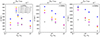Fig. 1. Scales of the radio sources, d, at different times (100 Myr, 300 Myr, and 500 Myr) varying with the jet powers. We determined the scales of the radio sources by doubling the distance from the heads of the one-sided radio lobes to the center of galaxy. The stars are color-coded to represent distinct fractions of energy components and the magnetic structure parameter, αp. The arrow indicates that the source is larger than the simulated region.

It is also interesting to see whether the lower power-larger bubble effect exists when considering the same radio power for different sources. In the left panel of Fig. 2, we present the scales of the radio sources varying with jet power, specifically at the instant when the sources have declined to radio power (luminosity) of 10²⁵ W Hz⁻¹ at 144 (1 + z) MHz for redshift z = 0.3. The methodology for calculating radio emission is detailed in Appendix C. Notably, we can see that the low-power jets result in larger radio sources. The corresponding time t₂₅ for the radio power of 10²⁵ W Hz⁻¹ in different runs are shown in the right panel of Fig. 2 (dots), and we can see they all occur after the jets are switched off (t₂₅ > t_jet). We also calculated the typical synchrotron cooling times for the toroidal magnetic field dominant runs at times t = t_jet and t = t₂₅. We can observe that, if the electrons cannot be adequately accelerated after the jets are switched off, they will quickly cool down, particularly for the high-power jets (upward triangles in the right panel of Fig. 2). This means that, the t₂₅ for the high-power jets (t_jet < 200 Myr or P_jet/P_fb > 0.25) might be overestimated and when considering synchrotron cooling, the high-power jets will actually result in even smaller radio sources for the same radio power.

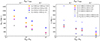Fig. 2. Scales of the radio sources, d25, at the radio power 1025 W Hz−1 (left) and the corresponding times (right), varying with the jet powers, Pjet, in simulations with diverse jet parameters, as listed in Table 1. The dots in the right panel represent the time t25 when the radio power of the source declines to 1025 W Hz−1. The horizontal lines in the right panel mark the time when the corresponding jet stops being powered, tjet. The triangles denote tjet + tsyn(tjet) (upward) and t25 + tsyn(t25) (downward), where tsyn(t) is the typical synchrotron cooling time at 144(1 + z) MHz for the volume-averaged magnetic field strength corresponding to the time t calculated using Eq. (C.11). The jet powers are normalized by the typical feedback power (bottom) and Eddington luminosity (top), as discussed in Sect. 2.3. The stars are color-coded to represent distinct fractions of energy components and the magnetic structure parameter, αp.

3.2. Behavior of the magnetic field

We also examined the impact of energy partition on the jet evolution. The results are presented in Fig. 2. Notably, jets dominated by toroidal magnetic energy (f_m = 0.8, α_p = 0.3) yield larger radio sources compared to those dominated by thermal or kinetic energy (f_m = 0.05, α_p = 0.3). This should be due to the magnetic tension force directed toward the jet axis (hoop stress), which can facilitate jet collimation, akin to mechanisms proposed to explain jet collimation near black holes (Romero & Vila 2014). This collimation results in slimmer lobes with reduced cross sections and lower drag forces during propagation through the ambient gas. Furthermore, in Fig. C.2 we can see that a stronger magnetic field shields the lobes from Kelvin-Helmholtz instability and minimizes mixing with the ambient gas (comparing runs t5, t5fth5, and t5fm8). Consequently, the magnetic field’s significance can also extend to explaining the bent radio sources observed in galaxy clusters, which are influenced by intra-cluster weather (Gan et al. 2017).

To study the effects of magnetic field structure in greater detail, we increased α_p from 0.3 to 3 in simulations where a strong magnetic field (f_m = 0.8) is injected. As shown in the runs with a stronger poloidal magnetic field (α_p = 3 in Fig. 2), the growth of radio lobes is effectively suppressed (see also Chen et al. 2023). This phenomenon is likely attributed to the reduced magnetic tension force directed toward the jet axis and the enhanced magnetic tension force toward the galaxy’s center within the lobe, resulting from the stronger poloidal magnetic field (α_p = 3).

3.3. Radio power of the simulated sources

Direct comparison between models and observations is challenging due to factors such as uncertainties of the properties of the nonthermal particles in lobes, the projection effect, and the quality of observed data (Hardcastle 2018). Nevertheless, as an approximation, we can gain some useful insights into the jet properties of GRSs by neglecting these details. The evolution of radio sources in the P-D diagram for all our simulations is presented in Fig. 3. Comparing Figs. 3 and 5, we can see that the radio powers decline significantly after the jet is switched off, and those produced by higher-power jets decline earlier. The data points in Fig. 3 represent the results of GRSs identified in clusters within the halo mass range of 0.7 − 2.0 × 10¹⁴ M_⊙, as observed in Dabhade et al. (2020b). It is clearly demonstrated that only the low-power jets (t_jet = 200 Myr) can readily traverse the observational region in the P-D diagram. A typical morphology of the radio sources produced by the low-power jets (run t200fm8) is shown in Fig. 4.

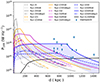Fig. 3. Evolution of the simulated radio sources in the P-D diagram. Distinct colors represent different powers, while different line styles signify distinct fractions of energy components and the magnetic structure parameter, αp. The blue shade covers regions with radio power one order of magnitude lower than that indicated by the solid blue line. The detailed methodology for calculating radio power is described in Appendix C. The data points utilized in this analysis are sourced from Dabhade et al. (2020b).

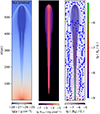Fig. 4. Snapshots of density (left panel), radio flux (middle panel), and magnetic field (right panel) for run t200fm8 at t = 250 Myr.

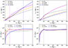Fig. 5. Evolution of the traveling distance of the heads of bubbles (upper panels) and the energy contained within the jetted bubbles (lower panels) in the two sets of runs discussed in Sects. 4.1 and 4.2. The bubble region is identified by a density lower than 5 × 10−27 g cm−3 and a toroidal magnetic field stronger than 10−9 G. The subsequent mixing between the bubble region and the ambient gas can result in an upward trend in the energy curves. Different line colors represent different runs. The vertical lines denote when the jets are shut off.

On the other hand, although jets with significantly lower power can generate much larger radio sources, they may be too faint to observe. As illustrated in Fig. 3, the evolution of the lowest-power jet (run t1200fm8, represented by the solid black line) barely reaches the lower boundary of the observational region. This result implies that the jet powers of these radio sources lie approximately within the range of 10⁻⁴ − 10⁻³L_Edd (the corresponding ratios of the jet powers to the Eddington luminosity are shown in Fig. 2). Furthermore, the jet active time of run t1200fm8 is approximately the typical synchrotron cooling time (Eq. (C.11)) of the electrons in the radio lobes; thus, the outer part of the lobes might be radio-dark if the new acceleration of electrons is not adequate. Considering the very low density and pressure of the extreme low-power jets, the mixing between ejecta and surrounding medium might even cause them fail to form low density bubbles or observable radio lobes.

4. Discussion

4.1. Energy transport processes

We examine energy transport processes in different runs before discussing in detail the production of large radio sources. We now focus on two sets of runs: the runs with the same energy fractions (f_m = 0.8, f_th = 0.05, α_p = 0.3) but different powers and the runs with the same power (t_jet = 50 Myr) but different energy fractions or magnetic field structure. The upper panels in Fig. 5 show the evolution of the distance that the jetted bubble traveled (half of the dimension of radio sources) in these two sets of runs. The evolution of the total energy residing in jetted bubbles is also shown in the lower panels of Fig. 5. As an approximation, the bubble region is identified by a density lower than 5 × 10⁻²⁷ g cm⁻³ and a toroidal magnetic field stronger than 10⁻⁹ G. The dotted vertical lines show when the fixed total energy has been injected and the jet is turned off in different runs. We can see the scales of the jetted bubbles generally shows positive correlation with the total energy left in the bubbles particularly for the jets with the same energy makeup but different active times (powers). Notably, the high-power jet (run t5fm8) expels energy more rapidly upon jet cessation, leaving less energy within the bubble, which impedes the growth of the radio sources. Actually the most high-power jets can transmit energy outward through more potent shocks compared to low-power jets, which rely on less potent processes such as sound waves and slow expansions (Tang & Churazov 2017; Bambic & Reynolds 2019; Duan & Guo 2020).

While neglecting the mixing processes, the energy outflow rate from the bubble should be equivalent to the power associated with the work done by the bubble on the surrounding medium via thermal pressure and Maxwell stress (magnetic pressure plus magnetic tension), as shown in Eq. (D.3). This power can be decomposed into three components: the thermal pressure power (P_out, th), magnetic pressure power (P_out, m1), and magnetic tension power (P_out, m2), which can be calculated as follows:

$$\begin{array}{c}\hfill P_{\mathrm{out},\mathrm{th}}={\displaystyle {\int }_{S_{\mathrm{bub}}}}p\mathbf{v}·d\mathbf{S},\end{array}$$(10)

$$\begin{array}{c}\hfill P_{\mathrm{out},m1}={\displaystyle {\int }_{S_{\mathrm{bub}}}}\frac{B^2}{2}\mathbf{v}·d\mathbf{S},\end{array}$$(11)

$$\begin{array}{c}\hfill P_{\mathrm{out},m2}=-{\displaystyle {\int }_{S_{\mathrm{bub}}}}\mathbf{v}·\mathbf{B}\mathbf{B}·d\mathbf{S}.\end{array}$$(12)

The Maxwell stress power can be expressed as P_out, m = P_out, m1 + P_out, m2. The evolution of thermal pressure power, Maxwell stress power and magnetic pressure power varying with the traveling distance of lobes is shown in Fig. 6. The magnetic tension power can be determined by the difference between the Maxwell stress power and the magnetic pressure power, which can be negative for some cases (for example, during the early stage of run t50fm8bp3, as shown in the right panel of Fig. 6). The thermal pressure power and Maxwell stress power in the higher-power jet runs are both higher than those in low-power jet runs at the inner regions of clusters, as shown in the left panel. This means that higher-power jets experience greater adiabatic losses in the inner regions of clusters, leaving less energy residing in the bubbles at later times, as discussed in the last paragraph. This should be related to the lower power-larger bubble effect. On the other hand, we can see that low-power jets can transport more energy outside in the outer region of clusters, as indicated by the left panel of Fig. 6. Different energy makeups of jets do not result in as prominent differences as different powers, as shown in the right panel of Fig. 6.

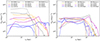Fig. 6. Thermal pressure power (solid lines), Maxwell stress power (dashed lines), and magnetic pressure power (dotted lines), calculated using Eqs. (10)–(12), varying with the traveling distance of lobes. Different colors represent the two sets of runs discussed in Sect. 4.1.

4.2. Production of large radio sources

To gain some insight into the production of large radio sources, we examined the evolution of the widths of the jetted bubbles and show the results in the upper panels of Fig. 7. We can see that, within the central region of the halos (for example, r < 100 kpc), the widths of the bubbles generally exhibit an anticorrelation with the ultimate extent of the simulated radio sources (see Figs. 1 and 5). Furthermore, we checked the volume-averaged internal pressure (magnetic pressure plus thermal pressure) within the bubbles and present the results in the lower panels of Fig. 7. We can see that internal pressures of bubbles show a positive correlation with the widths of bubbles in the innermost region of the halos. The dotted vertical lines show where the correlations have just begun to develop. This phenomenon is due to the fact that higher internal pressures within bubbles will cause faster transverse expansion, resulting in larger cross sections. The larger cross sections will make the jets much less penetrating and easier to be decelerated by the dense gas in the center of the halos. In the upper left panel of Fig. 7, we can observe that higher-power jets generally produce wider bubbles at the center of the halos. Subsequently, there will be stronger interactions between the higher-power jets and the surrounding gas, causing them to transfer more energy than low-power jets in the center of the halos, as discussed above.

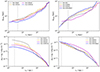Fig. 7. Width (upper panels) and volume-averaged internal pressure (including thermal and magnetic pressure; lower panels) of jetted bubbles varying with the traveling distance of the heads of bubbles in the two sets of runs discussed in Sects. 4.1 and 4.2. Different line colors represent different runs. The vertical lines denote the points where anticorrelations between the width (or pressure) and the final scales of the radio sources are beginning to develop.

We then checked the different results in runs t50fm8 and t50fm8bp3, which are injected with the same energy fractions and power but have different magnetic structures. As the emerging jet is far from equilibrium with the surrounding gas, it will undergo rapid changes in its properties. Before the identified low-density bubbles are established, the jet in run t50fm8 should have experienced fiercer expansion than the jet in run t50fm8bp3, so that it is wider at the innermost region, as shown in the upper right panel of Fig. 7. This also causes the thermal and kinetic energy density in the jet in run t50fm8 to be less than that in run t50fm8bp3, as shown in the right panel of Fig. C.1. The rapid expansion process might be due to the more prominent hoop effect of the stronger toroidal magnetic field in run t50fm8, as it will make the ejecta interact strongly with the dense gas in front of the jet at the center of the halos. Then, when the channel is open, the jet in run t50fm8 becomes slimmer than the jet in run t50fm8bp3.

On the other hand, the inflated bubbles with stronger poloidal magnetic field and thermal energy (runs t50fm8bp3 and t50fth8) also seem to experience stronger Kelvin-Helmholtz instability than the bubbles jetted by toroidal magnetic field dominant jets, as shown in Fig. C.2. This will make things more complicated, as the Kelvin-Helmholtz instability can trigger more prominent mixing with the surrounding medium. The mixing processes will actually make the low density bubbles lose more matter and energy than the stable ones, and finally reduce their potential to grow into large radio sources. This phenomenon is more pronounced in the case of higher-power jets, as illustrated in Fig. C.2. We will address more details regarding the relationship between the structure of the magnetic field and the Kelvin-Helmholtz instability in future studies.

4.3. Extended phenomena and limitations

The large-scale magnetic field within black hole accretion flows is pivotal for jet launching and collimation (Cao 2011; Chen & Zhang 2021; Li & Cao 2022). Our simulations underscore the criticality of the toroidal magnetic field at kiloparsec scales in initiating and confining giant radio jets/lobes, as discussed in Sect. 3.2. Additionally, the wake flows of AGN bubbles are essential for elucidating metal-rich outflows and cold filaments in galaxy clusters (Duan & Guo 2018, 2024). This study reveals that jetted bubbles can amplify the weak magnetic fields in the centers of clusters and ultimately result in stronger magnetic fields in their wake flows, as shown in Figs. 4 and C.2, which may contribute to the seeding of magnetic fields in the circumgalactic and intergalactic media at later stages.

The proportion of GRSs in galaxy clusters appears to be low (Dabhade et al. 2020b), suggesting their real-world formation may be challenging. In our simulations, with a fixed total injection energy, GRS formation is also contingent upon the total energy injection, and insufficient energy, even at the same power, will fail to yield GRSs. Our results suggest that a long-term stable jet output from the supermassive black hole’s accretion system is necessary for GRS production. Additionally, GRSs generated by excessively low-power jets (run t1200fm8) may be too dim for detection, as discussed in Sect. 3.3.

The morphology of GRSs is diverse in observations (Dabhade et al. 2020b), and thus a detailed comparison with our simulations is beyond the scope of this work. Nor do we apply intra-cluster weather effects in our simulations, which explains the bent radio lobes typically seen in clusters (Gan et al. 2017). We observe that many GRSs extend along the jet axis (Dabhade et al. 2020b), a feature readily replicated in our simulations, particularly with strong toroidal magnetic field injections (Figs. 4 and C.2). Another notable property is the significant decrease in radio flux at the edges in our simulations (middle panel, Fig. 4), consistent with observations of some large radio lobes (Wu et al. 2020). Furthermore, the gas environment can influence GRS morphology. For instance, in gas halos with lower baryon fractions, jetted lobes may expand more readily, adopting fatter shapes. We aim to delve into the effects of different gas environments in future studies. The velocity will also influence the morphology of radio sources. If higher velocities (for example, fully relativistic) of jets are considered, the density of the jets will be much lower for the same power or kinetic energy flux. This will render the jets less penetrating and produce flatter lobes, as demonstrated in English et al. (2016). On the other hand, full three-dimensional MHD simulations of jets may encounter kink instability (Mignone et al. 2010) and three-dimensional turbulence, both of which will pose difficulties for the growth of radio sources. The turbulence triggered by Kelvin-Helmholtz and Rayleigh-Taylor instabilities in two dimensions cannot experience the energy cascade to small scales as it does in three dimensions, which will result in different entrainment properties and morphologies of the jetted lobes (Massaglia et al. 2016).

5. Conclusions

We utilized MHD simulations to study the formation of GRSs within galaxy clusters. To avoid confusing the effects of power and total energy injection, we held the energy of jet outbursts fixed and studied the effect of power by varying the active duration of the jets. We also examined the roles of magnetic, thermal, and kinetic energy components by adjusting their fractions in the jets. Additionally, we calculated radio emission for comparison with observations in the P-D diagram. The main results are summarized as follows:

(i) Lower power-larger bubble effect. For a fixed total energy in jet outbursts, we present the scaling of radio source sizes varying with jet power, particularly at the instant when the sources have declined to a common radio power of 10²⁵ W Hz⁻¹ at 144(1 + z) MHz. We have found a trend that the jets with lower power yield larger radio sources.

(ii) Behavior of the magnetic field. When the energy is injected predominantly in the form of a toroidal magnetic field, the jets tend to produce larger radio sources. If instead the poloidal field injected is stronger, the growth of the radio lobes is suppressed.

(iii) P-D diagram. When injecting jet outbursts of E_jet = 2.06 × 10⁵⁹ erg into a halo of 10¹⁴ M_⊙, only jets with powers approximately within the range 10⁻⁴–10⁻³L_Edd and magnetic energy dominated by the toroidal component can readily traverse the observational region in the P-D diagram. Thus, our results suggest that energetic, long-term (low-power), continuous jets with significant kiloparsec-scale toroidal magnetic fields facilitate GRS formation in cluster environments. On the other hand, although the jets with significantly lower power can generate much larger radio sources, they may be too faint to be observable.

(iv) Energy transport processes. Higher-power jets generally produce jetted bubbles with higher internal pressure, which makes them wider and means they penetrate less into the centers of clusters, ultimately producing smaller radio sources. At the same time, higher-power jets expel energy more rapidly at the centers of galaxy clusters through adiabatic losses, resulting from the work done on the surrounding medium by thermal pressure and Maxwell stress. This process leaves less energy within the bubbles produced by higher-power jets, thereby impeding the growth of the radio sources.

We primarily focused on the impact of jet properties on the formation of GRSs within cluster environments. We did not delve into other potential factors that may influence the formation processes and properties of GRSs, such as the effects of different gas environments, the extreme relativistic ejecta, the three-dimensional turbulence, and the kink instability during jet propagation. We aim to comprehensively explore these effects in future studies.

Acknowledgments

We thank the anonymous referee for the constructive reports, particularly for the suggestions regarding the addition of discussions. This work was supported by the High Performance Computing Center of Henan Normal University. R.Z. was supported by the China Postdoctoral Science Foundation (No. 2023M731014). J.L. was supported by the NSFC (12303020), the Yunnan Fundamental Research Projects (NO.202401CF070169), and the Xingdian Talent Support Plan – Youth Project.

References

Appendix A: Gravitation and gas environment

We modified the models presented in Guo et al. (2018) and Fang et al. (2020) to establish the gravitational potential and gas environment for giant elliptical galaxies in galaxy clusters. For the dark matter gravitational potential, we adopted the Navarro–Frenk–White (NFW) profile (Navarro et al. 1997):

$$\begin{array}{c}\hfill {\mathrm{\Phi }}_{\text{dm}}=-\frac{2G{M}_0}{r_{}\text{s}}\frac{ln(1+r/r_{}\text{s})}{r/r_{}\text{s}}\end{array}$$(A.1)

Here, M₀ and r_s are determined by the virial mass of the dark matter halo M_vir, as follows:

$$\begin{array}{c}\hfill M_0=\frac{M_{\text{vir}}/2}{ln(1+C)-C/(1+C)},\end{array}$$(A.2)

$$\begin{array}{c}\hfill R_{\mathit{vir}}=206{\left(\frac{M_{\text{vir}}}{{10}^{12}{M}_{\odot }}\right)}^{1/3}\text{kpc},\end{array}$$(A.3)

$$\begin{array}{c}\hfill r_s=\frac{R_{\text{vir}}}{C}.\end{array}$$(A.4)

In this study, we adopted a concentration parameter C = 4.06 for a virial mass of M_vir = 10¹⁴ M_⊙ for the halo of clusters (typical value in Dabhade et al. 2020b).

The potential of the central galaxy (Hernquist 1990) is given by

$$\begin{array}{c}\hfill {\mathrm{\Phi }}_{\star }=-\frac{G{M}_{\star }}{r+a},\end{array}$$(A.5)

where M_⋆ represents the total stellar mass, and a = R_e/1.8153. Here, R_e denotes the radius of the isophote enclosing half of the galaxy’s light. The stellar mass M_⋆ is determined by the virial mass M_vir (Guo et al. 2010), as follows:

$$\begin{array}{c}\hfill M_{\star }=0.129M_{}\text{vir}{C}_M^{-2.44},\end{array}$$(A.6)

where C_M is defined as

$$\begin{array}{c}\hfill C_{}\text{M}={\left(\frac{M_{}\text{vir}}{2.5119\times {10}^{11}{M}_{\odot }}\right)}^{-0.926}+{\left(\frac{M_{}\text{vir}}{2.5119\times {10}^{11}{M}_{\odot }}\right)}^{0.261}.\end{array}$$(A.7)

The radius R_e is fitted from Jin et al. (2020) using the relation

$$\begin{array}{c}\hfill R_e(\text{kpc})={\left(\frac{0.186M_{\star }}{{10}^{10}{M}_{\odot }}\right)}^{1.116}+1.17.\end{array}$$(A.8)

For this work, we have M_⋆ ≈ 2.84 × 10¹¹ M_⊙ and R_e ≈ 7.59kpc.

The potential of the central black hole (Paczyńsky & Wiita 1980; Quataert & Narayan 2000) is given by

$$\begin{array}{c}\hfill {\mathrm{\Phi }}_{}\text{bh}=-\frac{G{M}_{}\text{bh}}{r-r_g},\end{array}$$(A.9)

where M_bh represents the black hole mass, and r_g = 2GM_bh/c² is the Schwarzschild radius. M_bh is determined by the stellar mass using the relation (Häring & Rix 2004)

$$\begin{array}{c}\hfill M_{}\text{bh}=1.6\times {10}^8{\left(\frac{M_{\star }}{{10}^{11}{M}_{\odot }}\right)}^{1.12}{M}_{\odot }.\end{array}$$(A.10)

For this work, we have M_bh ≈ 5.16 × 10⁸ M_⊙. The gravitational effect of the black hole is actually negligible in this work but not for the halo with higher mass (e.g., A1795); we include it here for consistency with future studies of larger halos.

We followed Fang et al. (2020) and Guo et al. (2020), with modifications, to set the distribution of the hot gas. The density profile of the gas is given by

$$\begin{array}{c}\hfill \rho (r)=\frac{M_{}\text{n}}{(r+R_{}\text{e}){(r+0.5R_{}\text{vir})}^2},\end{array}$$(A.11)

where M_n is a constant normalized by the total gas mass M_g within the virial radius, which is calculated as

$$\begin{array}{c}\hfill M_{}\text{g}={\displaystyle {\int }_{r_{}\text{min}}^{r_{}\text{vir}}}4\pi r^2\rho (r)dr.\end{array}$$(A.12)

The total gas mass M_g is determined by the virial mass of the dark matter halo and the gas fraction f_g as M_g = f_gM_vir. We adopted f_g ≈ 0.108, which corresponds to a baryon fraction of about 0.1 for galaxies with a halo mass of 10¹⁴ M_⊙, as indicated by observations (Vikhlinin et al. 2006; Li et al. 2018; Zhang et al. 2024). When the gravitation and density profile is determined, the initial temperature profile is set up according to the assumption of hydrostatic equilibrium: ρ∇Φ = −∇p and p = ρk_BT/(μm_p), with the mean molecular weight μ = 0.61. The temperature at the outer boundary is set as T_out = 0.5T_vir, where the virial temperature T_vir is

$$\begin{array}{c}\hfill T_{}\text{vir}={10}^6{\left(\frac{M_{}\text{vir}}{{10}^{12}{M}_{\odot }}\right)}^{2/3}K.\end{array}$$(A.13)

The profiles of density and temperature with different halo masses and baryon fractions are plotted in Fig. A.1. We can see for the halo mass of 7.06 × 10¹⁴ M_⊙, this model reproduce the result fitted from observation of galaxy cluster A1795 well (Guo et al. 2018).

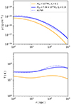Fig. A.1. Profiles of density and temperature for virial masses (Mvir) of 1014 M⊙ (solid orange lines, fb = 0.1, adopted in this work) and 7.06 × 1014 M⊙ (solid blue lines, fb = 0.14). The latter is contrasted with the fitting results of galaxy cluster A1795 (dashed blue line; Guo et al. 2018).

Appendix B: Injection of magnetic energy

We developed a straightforward method for regulating the injection of magnetic energy of jets. Following Mbarek & Caprioli (2019) with modifications, the toroidal magnetic field is set proportional to r inside the jet base, 1/r outside and zero further away, as given by

$$\begin{array}{c}\hfill B_{\text{inj},\varphi }=\{\begin{array}{c}\hfill B_0\frac{r}{R_0},\&\text{for}r<R_0\text{and}z<h_{\mathrm{jet}},\\ \hfill B_0\frac{R_0}{r},\&\text{for}{R}_0<r<2R_0\text{and}z<h_{\mathrm{jet}},\\ \hfill 0,\&\text{for}r>2R_0\text{or}z>h_{\mathrm{jet}},\\ \hfill \end{array}\end{array}$$(B.1)

where R₀ and h_jet are the cross-sectional radius and height of the jet base, respectively. Following Li et al. (2006) and Gan et al. (2017), the poloidal magnetic field components are defined as

$$\begin{array}{c}\hfill B_{\text{inj},z}={\alpha }_p{B}_0·2(1-\frac{r^2}{R_0^2})exp(-\frac{r^2+z^2}{R_0^2}),\end{array}$$(B.2)

$$\begin{array}{c}\hfill B_{\text{inj},r}={\alpha }_p{B}_0·\frac{2zr}{R_0^2}exp(-\frac{r^2+z^2}{R_0^2}),\end{array}$$(B.3)

where α_p is the parameter of the magnetic field structure that determines the ratio between the poloidal and toroidal magnetic fields. The poloidal magnetic field is injected throughout the entire simulation region, although its value is negligible for cells far from the jet base. It is straightforward to prove that this magnetic field configuration satisfies ∇ ⋅ B = 0 analytically in cylindrical coordinates. Then, the injection rate of magnetic energy can be expressed as

$$\begin{array}{c}\hfill {\dot{e}}_{\text{b},\varphi }=\{\begin{array}{c}\hfill \frac{1}{2}{\dot{e}}_{b0}\frac{r^2}{R_0^2},\&\text{for}r<R_0\text{and}z<h_{\mathrm{jet}},\\ \hfill \frac{1}{2}{\dot{e}}_{b0}\frac{R_0^2}{r^2},\&\text{for}{R}_0<r<2R_0\text{and}z<h_{\mathrm{jet}},\\ \hfill 0,\&\text{for}r>2R_0\text{or}z>h_{\mathrm{jet}},\\ \hfill \end{array}\end{array}$$(B.4)

$$\begin{array}{c}\hfill {\dot{e}}_{\text{b},z}=\frac{1}{2}{\alpha }_p^2{\dot{e}}_{b0}·4{(1-\frac{r^2}{R_0^2})}^{2}exp(-2\frac{r^2+z^2}{R_0^2}),\end{array}$$(B.5)

$$\begin{array}{c}\hfill {\dot{e}}_{\text{b},r}=\frac{1}{2}{\alpha }_p^2{\dot{e}}_{b0}·\frac{4z^2{r}^2}{R_0^4}exp(-2\frac{r^2+z^2}{R_0^2}),\end{array}$$(B.6)

where ${\dot{e}}_{b0}=\frac{d}{\mathit{dt}}(B_0^2)$. The power of magnetic energy injection is defined as

$$\begin{array}{c}\hfill \begin{array}{cc}\hfill P_{}\text{m}& ={\displaystyle {\int }_V}({\dot{e}}_{\text{b},\varphi }+{\dot{e}}_{\text{b},z}+{\dot{e}}_{\text{b},r})dV\hfill \\ \hfill & =[(\frac{1}{4}+\text{ln}2)\pi h_{\mathrm{jet}}{R}_0^2+\frac{5\pi }{16}\sqrt{\frac{\pi }{2}}{\alpha }_p^2{R}_0^3]{\dot{e}}_{b0}.\hfill \end{array}\end{array}$$(B.7)

We maintained this magnetic power as a fraction (f_m) of the total injection power, given by

$$\begin{array}{c}\hfill P_{}\text{m}=f_{}\text{m}{P}_{}\text{inj}.\end{array}$$(B.8)

The value of ė_b0 can be determined by combining Eqs. B.7 and B.8. Then, using Eqs. B.4 - B.6, the injection rate of magnetic energy can be solved for all regions. The magnitude of magnetic field is updated via the equation

$$\begin{array}{c}\hfill \frac{\partial B_i^2}{\partial t}=2{\dot{e}}_{\text{b},i},\end{array}$$(B.9)

where i represents ϕ, z or r. This means that the difference form of the injection rate of the magnetic field can be expressed as

$$\begin{array}{c}\hfill \frac{B_i(t+\mathrm{\Delta }t)-B_i(t)}{\mathrm{\Delta }t}\approx \frac{\pm {[B_i^2(t)+2{\dot{e}}_{\text{b},i}\mathrm{\Delta }t]}^{\frac{1}{2}}-B_i(t)}{\mathrm{\Delta }t}.\end{array}$$(B.10)

The sign ± is controlled to be consistent with Eqs. B.1-B.3, which means B_z is injected positively at r < R₀ and negatively at r > R₀, whereas B_ϕ and B_r are both injected positively throughout the entire injection region. This method enables us to control the fraction of magnetic energy injected into the system, which is crucial for our work. To be consistent with Eq.4, Eq. B.9 would require

$$\begin{array}{c}\hfill {\dot{B}}_{\text{inj},i}=\frac{{\dot{e}}_{\text{b},i}}{B_i}.\end{array}$$(B.11)

Appendix C: Calculation of synchrotron radiation

Similar to some previous works, we calculated the radio emission using post-processing methods (Hardcastle & Krause 2014; Yates et al. 2018). Assuming the distribution of nonthermal electrons within the radio sources follows

$$\begin{array}{c}\hfill N(\gamma )=N_0{\gamma }^{-q},\end{array}$$(C.1)

where γ is the Lorentz factor and q is the spectral index of the electrons. The spectral emission coefficient for synchrotron radiation is given by (Ginzburg & Syrovatskii 1965; Rybicki & Lightman 1979)

$$\begin{array}{c}\hfill j_{\nu }=f(q)\frac{\sqrt{3}}{4\pi }\frac{e^3{N}_0}{m_e{c}^2}{\left(\frac{2\pi m_{e}c\nu }{3e}\right)}^{-\frac{q-1}{2}}{(Bsin{\theta }_p)}^{\frac{q+1}{2}},\end{array}$$(C.2)

where θ_p is the pitch angle of the electrons, and

$$\begin{array}{c}\hfill f(q)=\frac{1}{q+1}\mathrm{\Gamma }(\frac{q}{4}+\frac{19}{12})\mathrm{\Gamma }(\frac{q}{4}-\frac{1}{12}).\end{array}$$(C.3)

As an approximation, the distributions of electrons and radiation are typically assumed to be locally isotropic, allowing the emission coefficient to be expressed as

$$\begin{array}{c}\hfill j_{\nu }=a(q)\frac{\sqrt{3}}{4\pi }\frac{e^3{N}_0}{m_e{c}^2}{\left(\frac{2\pi m_{e}c\nu }{3e}\right)}^{-\frac{q-1}{2}}{B}^{\frac{q+1}{2}},\end{array}$$(C.4)

where

$$\begin{array}{c}\hfill a(q)=\frac{\sqrt{\pi }}{2}\mathrm{\Gamma }\left(\frac{q+5}{4}\right){\left[\mathrm{\Gamma }\left(\frac{q+7}{4}\right)\right]}^{-1}f(q).\end{array}$$(C.5)

The radiation exhibits a spectral distribution of j_ν ∼ ν^−α with α = (q − 1)/2. We adopted α = 0.7, a typical value in the observation (Dabhade et al. 2023). Given that the magnetic field can be derived from our simulations, the only unknown parameter is N₀ in Eq. C.1. According to Eq. C.1, the energy density of nonthermal electrons is given by

$$\begin{array}{c}\hfill u_e={\displaystyle {\int }_{{\gamma }_{\text{min}}}^{{\gamma }_{\text{max}}}}N(\gamma )\gamma m_e{c}^{2}d\gamma .\end{array}$$(C.6)

Thus, N₀ can be determined as follows:

$$\begin{array}{c}\hfill N_0=\{\begin{array}{ccc}& \frac{u_e}{m_e{c}^2}ln(\frac{{\gamma }_{}\text{min}}{{\gamma }_{}\text{max}})\hfill & \hfill ,q=2\\ \hfill \\ \hfill & \frac{u_e}{m_e{c}^2}\frac{2-q}{{\gamma }_{\mathit{max}}^{(2-q)}-{\gamma }_{\mathit{min}}^{(2-q)}}\hfill & \hfill ,q\ne 2.\\ \hfill \end{array}\end{array}$$(C.7)

Here, γ_min and γ_max are empirically set to 100 and 10⁵, respectively (Hardcastle & Krause 2014; Hardcastle 2018). We assumed that u_e is a fraction η_e of the non-magnetized energy, defined as

$$\begin{array}{c}\hfill u_e={\eta }_e(e-\frac{B^2}{2}),\end{array}$$(C.8)

where e represents the total energy density in Eq. 3. For self-consistency, we adopted η_e = 0.1 as we expect the nonthermal electrons to have negligible impact on the dynamics of the jets and lobes in our simulations. Finally, N₀ can be derived from Eqs. C.7 and C.8. In Fig. C.1 we show the volume-averaged energy density of various energy components varying with the traveling distance of the lobes.

The radio power (luminosity) of radio sources can be calculated as

$$\begin{array}{c}\hfill P_{\nu }={\displaystyle {\int }_V}4\pi j_{\nu }dV.\end{array}$$(C.9)

The radio flux can be determined by

$$\begin{array}{c}\hfill \mathrm{\Delta }F={\displaystyle {\int }_{l_{-}}^{l_{+}}}{j}_{\nu }dl·\frac{\mathrm{\Delta }A}{d_L^2},\end{array}$$(C.10)

where l₋ − l₊ represents the integral path traversing the radio sources along the line of sight perpendicular to the jet axis. ΔA denotes the cross-sectional area of the simulation cells along the line of sight, and d_L is the luminosity distance. For this study, we place the sources in our simulations at a redshift of z = 0.3 (typical value of the sources in Dabhade et al. 2020b) and calculate the radio power and flux at frequency ν = 144(1 + z)MHz. The radiating lobe region is identified by a density lower than 5 × 10⁻²⁷ g cm⁻³ and a toroidal magnetic field stronger than 10⁻⁹ G. In Figs. 4 and C.2, we present snapshots of the radio flux distribution of the sources from selected runs, alongside the corresponding distributions of density and magnetic field.

The synchrotron cooling time of electrons in the radio lobes of AGNs is typically hundreds of million years (Ghisellini 2013). The cooling time at a certain frequency (Courvoisier 2013) can be estimated as

$$\begin{array}{c}\hfill t_{\mathrm{syn}}(s)\approx 6\times {10}^8{B}_{\mathrm{G}}^{-3/2}{\nu }_{\mathrm{MHz}}^{-1/2}.\end{array}$$(C.11)

For the frequency of ν = 144(1+0.3)MHz, Eq. C.11 results in a cooling time of about 43.9 Myr for a magnetic field of 10⁻⁵ G and 1.4 Gyr for 10⁻⁶ G, which means the electrons will undergo significant synchrotron cooling if the magnetic field is sufficiently strong when the jets are shut off.

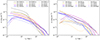Fig. C.1. Volume-averaged energy density of different energy components varying with the traveling distance of lobes in the two sets of runs discussed in Sect. 4.2. Different colors represent different runs, whereas the dotted, dashed, and solid lines signify kinetic, thermal, and magnetic energy densities, respectively.

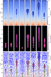Fig. C.2. Snapshots of density (top), radio flux (middle), and magnetic field (bottom) for runs with tjet = 5Myr and tjet = 50Myr at t = 300Myr. The pixel sizes in the radio flux plots directly mirror the cell sizes employed in the simulations.

Appendix D: Integral energy equation in Lagrangian form

Here we consider the energy loss from a given jetted bubble as it interacts with the surrounding medium. The energy equation, Eq. 3, can be written in its full conservation form, as usually shown in textbooks (Ogilvie 2016). Omitting the jet injection, we have

$$\begin{array}{c}\hfill \frac{\partial }{\partial t}(e+\rho \mathrm{\Phi })+\mathrm{\nabla }·[(e+\rho \mathrm{\Phi })\mathbf{v}+(p+\frac{B^2}{2})\mathbf{v}-\mathbf{B}\mathbf{B}·\mathbf{v}]=0.\end{array}$$(D.1)

When considering the energy outflow from a moving and growing bubble, we must refer to the integral energy equation in Lagrangian form. While neglecting the mixing processes, the energy outflow rate from the region V_bub of the given bubble can be written as

$$\begin{array}{c}\hfill \begin{array}{cc}\hfill P_{\mathit{out}}& =-\frac{d}{\mathit{dt}}{\displaystyle {\int }_{V_{\mathit{bub}}}}(e+\rho \mathrm{\Phi })dV\hfill \\ \hfill & =-{\displaystyle {\int }_{V_{\mathit{bub}}}}[\frac{d}{\mathit{dt}}(e+\rho \mathrm{\Phi })+(e+\rho \mathrm{\Phi })\mathrm{\nabla }·\mathbf{v}]dV\hfill \\ \hfill & =-{\displaystyle {\int }_{V_{\mathit{bub}}}}\{\frac{\partial }{\partial t}(e+\rho \mathrm{\Phi })+\mathrm{\nabla }·[(e+\rho \mathrm{\Phi })\mathbf{v}]\}dV.\hfill \end{array}\end{array}$$(D.2)

Here we have used the relation between the rate of change of a small volume and velocity $\frac{1}{\mathrm{\Delta }V}\frac{d\mathrm{\Delta }V}{\mathit{dt}}=\mathrm{\nabla }·\mathbf{v}$ and the relation between Lagrangian and Eulerian derivatives $\frac{d}{\mathit{dt}}=\frac{\partial }{\partial t}+\mathbf{v}·\mathrm{\nabla }$ (or applying the Reynolds Transport Theorem). Then, using Eq. D.1, we have

$$\begin{array}{c}\hfill P_{\mathit{out}}={\displaystyle {\int }_{S_{\mathit{bub}}}}[(p+\frac{B^2}{2})\mathbf{v}-\mathbf{v}·\mathbf{B}\mathbf{B}]·d\mathbf{S},\end{array}$$(D.3)

where S_bub is the surface of the bubble. The physical meaning is obvious: the bubble mainly loses energy through adiabatic processes due to the work done by the thermal pressure and Maxwell stress tensor (magnetic pressure plus magnetic tension). The same derivation for the mass equation results in a zero mass loss rate, indicating the mass conservation in the moving bubbles when the mixing processes are neglected.

All Tables

All Figures

Fig. 1. Scales of the radio sources, d, at different times (100 Myr, 300 Myr, and 500 Myr) varying with the jet powers. We determined the scales of the radio sources by doubling the distance from the heads of the one-sided radio lobes to the center of galaxy. The stars are color-coded to represent distinct fractions of energy components and the magnetic structure parameter, αp. The arrow indicates that the source is larger than the simulated region.

In the text

Fig. 2. Scales of the radio sources, d25, at the radio power 1025 W Hz−1 (left) and the corresponding times (right), varying with the jet powers, Pjet, in simulations with diverse jet parameters, as listed in Table 1. The dots in the right panel represent the time t25 when the radio power of the source declines to 1025 W Hz−1. The horizontal lines in the right panel mark the time when the corresponding jet stops being powered, tjet. The triangles denote tjet + tsyn(tjet) (upward) and t25 + tsyn(t25) (downward), where tsyn(t) is the typical synchrotron cooling time at 144(1 + z) MHz for the volume-averaged magnetic field strength corresponding to the time t calculated using Eq. (C.11). The jet powers are normalized by the typical feedback power (bottom) and Eddington luminosity (top), as discussed in Sect. 2.3. The stars are color-coded to represent distinct fractions of energy components and the magnetic structure parameter, αp.

In the text

Fig. 3. Evolution of the simulated radio sources in the P-D diagram. Distinct colors represent different powers, while different line styles signify distinct fractions of energy components and the magnetic structure parameter, αp. The blue shade covers regions with radio power one order of magnitude lower than that indicated by the solid blue line. The detailed methodology for calculating radio power is described in Appendix C. The data points utilized in this analysis are sourced from Dabhade et al. (2020b).

In the text

	Fig. 4. Snapshots of density (left panel), radio flux (middle panel), and magnetic field (right panel) for run t200fm8 at t = 250 Myr.
In the text

Fig. 5. Evolution of the traveling distance of the heads of bubbles (upper panels) and the energy contained within the jetted bubbles (lower panels) in the two sets of runs discussed in Sects. 4.1 and 4.2. The bubble region is identified by a density lower than 5 × 10−27 g cm−3 and a toroidal magnetic field stronger than 10−9 G. The subsequent mixing between the bubble region and the ambient gas can result in an upward trend in the energy curves. Different line colors represent different runs. The vertical lines denote when the jets are shut off.

In the text

	Fig. 6. Thermal pressure power (solid lines), Maxwell stress power (dashed lines), and magnetic pressure power (dotted lines), calculated using Eqs. (10)–(12), varying with the traveling distance of lobes. Different colors represent the two sets of runs discussed in Sect. 4.1.
In the text

Fig. 7. Width (upper panels) and volume-averaged internal pressure (including thermal and magnetic pressure; lower panels) of jetted bubbles varying with the traveling distance of the heads of bubbles in the two sets of runs discussed in Sects. 4.1 and 4.2. Different line colors represent different runs. The vertical lines denote the points where anticorrelations between the width (or pressure) and the final scales of the radio sources are beginning to develop.

In the text

	Fig. A.1. Profiles of density and temperature for virial masses (Mvir) of 1014 M⊙ (solid orange lines, fb = 0.1, adopted in this work) and 7.06 × 1014 M⊙ (solid blue lines, fb = 0.14). The latter is contrasted with the fitting results of galaxy cluster A1795 (dashed blue line; Guo et al. 2018).
In the text

	Fig. C.1. Volume-averaged energy density of different energy components varying with the traveling distance of lobes in the two sets of runs discussed in Sect. 4.2. Different colors represent different runs, whereas the dotted, dashed, and solid lines signify kinetic, thermal, and magnetic energy densities, respectively.
In the text

	Fig. C.2. Snapshots of density (top), radio flux (middle), and magnetic field (bottom) for runs with tjet = 5Myr and tjet = 50Myr at t = 300Myr. The pixel sizes in the radio flux plots directly mirror the cell sizes employed in the simulations.
In the text

References

- Baldwin, J. E. 1982, in Extragalactic Radio Sources, eds. D. S. Heeschen, & C. M. Wade, IAU Symp., 97, 21 [NASA ADS] [Google Scholar]
- Bambic, C. J., & Reynolds, C. S. 2019, ApJ, 886, 78 [NASA ADS] [CrossRef] [Google Scholar]
- Cao, X. 2011, ApJ, 737, 94 [NASA ADS] [CrossRef] [Google Scholar]
- Chen, L., & Zhang, B. 2021, ApJ, 906, 105 [NASA ADS] [CrossRef] [Google Scholar]
- Chen, Y.-H., Heinz, S., & Hooper, E. 2023, MNRAS, 522, 2850 [Google Scholar]
- Courvoisier, T. J. L. 2013, High Energy Astrophysics: An Introduction (Berlin Heidelberg: Springer-Verlag) [CrossRef] [Google Scholar]
- Dabhade, P., Mahato, M., Bagchi, J., et al. 2020a, A&A, 642, A153 [NASA ADS] [CrossRef] [EDP Sciences] [Google Scholar]
- Dabhade, P., Röttgering, H. J. A., Bagchi, J., et al. 2020b, A&A, 635, A5 [NASA ADS] [CrossRef] [EDP Sciences] [Google Scholar]
- Dabhade, P., Saikia, D. J., & Mahato, M. 2023, JApA, 44, 13 [NASA ADS] [Google Scholar]
- Davis, S. W., & Tchekhovskoy, A. 2020, ARA&A, 58, 407 [Google Scholar]
- Duan, X., & Guo, F. 2018, ApJ, 861, 106 [NASA ADS] [CrossRef] [Google Scholar]
- Duan, X., & Guo, F. 2020, ApJ, 896, 114 [Google Scholar]
- Duan, X., & Guo, F. 2024, ApJ, 972, 41 [Google Scholar]
- English, W., Hardcastle, M. J., & Krause, M. G. H. 2016, MNRAS, 461, 2025 [NASA ADS] [CrossRef] [Google Scholar]
- English, W., Hardcastle, M. J., & Krause, M. G. H. 2019, MNRAS, 490, 5807 [Google Scholar]
- Fang, X.-E., Guo, F., & Yuan, Y.-F. 2020, ApJ, 894, 1 [Google Scholar]
- Gan, Z., Li, H., Li, S., & Yuan, F. 2017, ApJ, 839, 14 [Google Scholar]
- Ghisellini, G. 2013, Radiative Processes in High Energy Astrophysics (Springer International Publishing Switzerland) [Google Scholar]
- Ginzburg, V. L., & Syrovatskii, S. I. 1965, ARA&A, 3, 297 [Google Scholar]
- Guo, F. 2015, ApJ, 803, 48 [Google Scholar]
- Guo, F. 2020, ApJ, 903, 3 [Google Scholar]
- Guo, Q., White, S., Li, C., & Boylan-Kolchin, M. 2010, MNRAS, 404, 1111 [NASA ADS] [Google Scholar]
- Guo, F., Duan, X., & Yuan, Y.-F. 2018, MNRAS, 473, 1332 [NASA ADS] [CrossRef] [Google Scholar]
- Guo, F., Zhang, R., & Fang, X.-E. 2020, ApJ, 904, L14 [Google Scholar]
- Hardcastle, M. J. 2018, MNRAS, 475, 2768 [Google Scholar]
- Hardcastle, M. J., & Krause, M. G. H. 2014, MNRAS, 443, 1482 [NASA ADS] [CrossRef] [Google Scholar]
- Häring, N., & Rix, H.-W. 2004, ApJ, 604, L89 [Google Scholar]
- Hernquist, L. 1990, ApJ, 356, 359 [Google Scholar]
- Jin, Y., Zhu, L., Long, R. J., et al. 2020, MNRAS, 491, 1690 [NASA ADS] [Google Scholar]
- Keppens, R., Meliani, Z., van Marle, A. J., et al. 2012, J. Comput. Phys., 231, 718 [Google Scholar]
- Lan, T.-W., & Prochaska, J. X. 2021, MNRAS, 502, 5104 [Google Scholar]
- Li, J.-W., & Cao, X. 2022, ApJ, 926, 11 [Google Scholar]
- Li, H., Lapenta, G., Finn, J. M., Li, S., & Colgate, S. A. 2006, ApJ, 643, 92 [NASA ADS] [CrossRef] [Google Scholar]
- Li, J.-T., Bregman, J. N., Wang, Q. D., Crain, R. A., & Anderson, M. E. 2018, ApJ, 855, L24 [NASA ADS] [CrossRef] [Google Scholar]
- Massaglia, S., Bodo, G., Rossi, P., Capetti, S., & Mignone, A. 2016, A&A, 596, A12 [NASA ADS] [CrossRef] [EDP Sciences] [Google Scholar]
- Mbarek, R., & Caprioli, D. 2019, ApJ, 886, 8 [NASA ADS] [CrossRef] [Google Scholar]
- McNamara, B. R., Kazemzadeh, F., Rafferty, D. A., et al. 2009, ApJ, 698, 594 [NASA ADS] [CrossRef] [Google Scholar]
- Meier, D. L. 1999, ApJ, 522, 753 [Google Scholar]
- Mignone, A., Rossi, P., Bodo, G., Ferrari, A., & Massaglia, S. 2010, MNRAS, 402, 7 [NASA ADS] [CrossRef] [Google Scholar]
- Mostert, R. I. J., Oei, M. S. S. L., Barkus, B., et al. 2024, A&A, 691, A185 [NASA ADS] [CrossRef] [EDP Sciences] [Google Scholar]
- Navarro, J. F., Frenk, C. S., & White, S. D. M. 1997, ApJ, 490, 493 [Google Scholar]
- Oei, M. S. S. L., van Weeren, R. J., Gast, A. R. D. J. G. I. B., et al. 2023, A&A, 672, A163 [NASA ADS] [CrossRef] [EDP Sciences] [Google Scholar]
- Oei, M. S. S. L., Hardcastle, M. J., Timmerman, R., et al. 2024a, Nature, 633, 537 [NASA ADS] [CrossRef] [Google Scholar]
- Oei, M. S. S. L., van Weeren, R. J., Hardcastle, M. J., et al. 2024b, A&A, 686, A137 [NASA ADS] [CrossRef] [EDP Sciences] [Google Scholar]
- Ogilvie, G. I. 2016, J. Plasma Phys., 82, 205820301 [Google Scholar]
- Paczyńsky, B., & Wiita, P. J. 1980, A&A, 88, 23 [NASA ADS] [Google Scholar]
- Quataert, E., & Narayan, R. 2000, ApJ, 528, 236 [Google Scholar]
- Romero, G. E., & Vila, G. S. 2014, Introduction to Black Hole Astrophysics (Berlin Heidelberg: Springer-Verlag) [CrossRef] [Google Scholar]
- Rybicki, G. B., & Lightman, A. P. 1979, Radiative Processes in Astrophysics (John Wiley and Sons, Inc.) [Google Scholar]
- Sankhyayan, S., & Dabhade, P. 2024, A&A, 687, L8 [NASA ADS] [CrossRef] [EDP Sciences] [Google Scholar]
- Tang, X., & Churazov, E. 2017, MNRAS, 468, 3516 [Google Scholar]
- Tang, H., Scaife, A. M. M., Wong, O. I., et al. 2020, MNRAS, 499, 68 [Google Scholar]
- Tchekhovskoy, A. 2015, in The Formation and Disruption of Black Hole Jets, eds. I. Contopoulos, D. Gabuzda, & N. Kylafis, Astrophys. Space Sci. Lib., 414, 45 [NASA ADS] [Google Scholar]
- Vikhlinin, A., Kravtsov, A., Forman, W., et al. 2006, ApJ, 640, 691 [Google Scholar]
- Wu, L.-H., Wu, Q.-W., Feng, J.-C., Lu, R.-S., & Fan, X.-L. 2020, RAA, 20, 122 [Google Scholar]
- Xia, C., Teunissen, J., El Mellah, I., Chané, E., & Keppens, R. 2018, ApJS, 234, 30 [Google Scholar]
- Yates, P. M., Shabala, S. S., & Krause, M. G. H. 2018, MNRAS, 480, 5286 [Google Scholar]
- Yuan, F., & Narayan, R. 2014, ARA&A, 52, 529 [NASA ADS] [CrossRef] [Google Scholar]
- Yuan, F., Yoon, D., Li, Y.-P., et al. 2018, ApJ, 857, 121 [Google Scholar]
- Zhang, Y., Comparat, J., Ponti, G., et al. 2024, A&A, 690, A267 [NASA ADS] [CrossRef] [EDP Sciences] [Google Scholar]