© The Authors 2025

1. Introduction

Planet formation is a multi-scale multi-physics process. The micro-physics of dust grain dynamics and cohesion, the long-range gravitational torques from the disk, and the intermediate-range physics of turbulence and aerodynamic drag are all key ingredients that must be studied and understood. These processes are usually studied in isolation, and we often struggle to understand the interactions between them. In this work we explore the interaction between two of these processes: grain growth by coagulation (e.g., Birnstiel et al. 2012) and the streaming instability (SI, Youdin & Goodman 2005; Johansen & Youdin 2007; Youdin & Johansen 2007). We seek to understand how they combine to form the ∼100 km primordial bodies that we call planetesimals, which are thought to be the building blocks of terrestrial planets and giant planet cores (Kokubo & Ida 1996, 2000).

The streaming instability (SI) (Youdin & Goodman 2005) is a convergence of radial drift among solid grains. It is perhaps the leading candidate for an explanation of how planetesimals form. While the details are complex, its qualitative behavior is simple enough. As dust grains feel gas drag, they also push back on the gas, and this feedback causes radially drifting grains to converge into azimuthal filaments. If these filaments reach the Hill density

$$\begin{array}{c}\hfill {\rho }_{\mathrm{R}}=\frac{9{\mathrm{\Omega }}_{\mathrm{K}}^2}{4\pi G},\end{array}$$(1)

where Ω_K is the Keplerian frequency and G is the gravitational constant, then the particle cloud may collapse gravitationally.

Much of the interest in the SI is driven by the evidence that seems to favor it. The sizes of present-day asteroids and the cratering record of Vesta (Morbidelli et al. 2009), along with the large number of equal-size Kuiper belt binaries (Nesvorný et al. 2010; Fraser et al. 2017), suggests that planetesimals formed through the gravitational collapse of a dust cloud. Gravitational collapse is also a natural mechanism to overcome dust growth barriers including the fragmentation and radial drift barriers (Güttler et al. 2010; Birnstiel et al. 2010) The SI in particular can reproduce the obliquities of trans-Neptunian binaries (Nesvorný et al. 2019) as well as the densities of Kuiper belt objects (Cañas et al. 2024).

However, the major challenge facing the SI (and a reason to be cautious about it) is that the conditions needed to trigger the SI (Carrera et al. 2015; Yang et al. 2017; Li & Youdin 2021; Lim et al. 2024a,b) are inconsistent with dust growth and disk evolution models as it requires fairly large grains and/or a high column dust-to-gas ratio Z in order to form filaments dense enough to reach the Hill density. Importantly, most studies of the SI criterion rely on 2D models without external turbulence. Lim et al. (2024a) showed that even a modest degree of external turbulence can make the critical Z much higher than those turbulence-free 2D models suggest. In this paper we make the case that dust coagulation is the missing ingredient that allows the SI to work with realistic turbulence.

In this paper we explore a simple hypothesis: that the SI and dust growth boost each other in a positive feedback. The SI leads to enhanced dust concentration, which reduces turbulence and radial drift. This, in turn, boosts grain growth, which then leads to a stronger, more efficient SI. If our hypothesis is correct, the combination of the SI and dust growth may be the key ingredient that makes planetesimal formation possible. Following a similar thought process, Johansen et al. (2009) showed that the SI dampens turbulence, Tominaga & Tanaka (2023) showed that SI filaments promote dust growth, and Ho et al. (2024) showed that dust growth can trigger the SI. We posit that there is, in fact, a feedback loop between dust growth and the SI, so that the two processes boost each other far beyond what might appear from studying just one interaction or the other.

This paper is organized as follows. Most of this manuscript consists of the presentation of the model in Sect. 2, where we derive the detailed relationships between the SI, mass loading, turbulence, and radial drift. In Sect. 3 we put these ingredients together to obtain our final results. We discuss in Sect. 4 and conclude in Sect. 5.

2. Model ingredients

2.1. How the SI boosts mass loading

Perhaps the best-known feature of the SI, and the reason it has garnered so much attention, is its ability to collect solid grains into dense filaments. We repurposed the dataset of Lim et al. (2024a), who conducted a large number of 3D simulations of the SI with external (i.e., forced) turbulence for St ∈ [0.01, 0.1], Z ∈ [0.015, 0.4], and α ∈ [10⁻⁴, 10⁻³], where St ≡ t_stopΩ_K is the grain’s Stokes number, Z = Σ_p/Σ_g is the column dust-to-gas ratio, and α is the squared Mach number of the turbulence. We calculated the typical dust-to-gas ratio ϵ inside the SI filaments and fit a power law. The details of this procedure are included in Appendix A, but the final result is that 55–80% of the grains in an SI filament experience a dust-to-gas ratio at least as high as

$$\begin{array}{c}\hfill {ϵ}_{\mathrm{SI}}\approx 1.12{\left(\frac{Z}{0.01}\right)}^{2.65}{\left(\frac{\mathrm{St}}{0.1}\right)}^{1.42}{\left(\frac{\alpha }{{10}^{-4}}\right)}^{-1.38}.\end{array}$$(2)

This equation was obtained from simulations in the range of (Z, St, α) described above. In this work we keep (St, α) within that range, but in 2 out of our 20 models we do extrapolate to Z = 0.0137 and 0.0118 (Sect. 3.1).

2.2. How mass loading boosts St_frag

The approach commonly used in the literature is to think of the gas-dust mixture as a single fluid, taking the limit St → 0 so that the mixture represents a colloidal suspension. In this limit, one thinks of the dust as contributing to the inertia of the fluid, but not to its pressure (Chang & Oishi 2010; Shi & Chiang 2013; Laibe & Price 2014; Lin & Youdin 2017; Chen & Lin 2018). This can be expressed as an “effective” sound speed

$$\begin{array}{cc}\hfill P& ={\rho }_{\mathrm{g}}{c}_{\mathrm{s}}^2=({\rho }_{\mathrm{g}}+{\rho }_{\mathrm{p}}){\stackrel{\sim }{c}}_{\mathrm{s}}^2,\hfill \\ \hfill {\stackrel{\sim }{c}}_{\mathrm{s}}& \equiv \frac{c_{\mathrm{s}}}{\sqrt{1+ϵ}},\hfill \end{array}$$

where ${\stackrel{\sim }{c}}_{\mathrm{s}}$ is the effective sound speed of the colloid.

However, in this work we are explicitly interested in the case where St may not be negligible, and the fluid might not be well represented by a colloid. Therefore, we take a different approach. We posit that turbulence is generated by a finite energy source that has to be partitioned between the gas and dust components

$$\begin{array}{cc}\hfill E& =\frac{1}{2}{\rho }_{\mathrm{g}}{v}_{\mathrm{g}}^2+\frac{1}{2}{\rho }_{\mathrm{p}}{v}_{\mathrm{p}}^2\hfill \\ \hfill & =\frac{1}{2}{\rho }_{\mathrm{g}}{v}_{\mathrm{g}}^2(1+ϵ\frac{v_{\mathrm{p}}^2}{v_{\mathrm{g}}^2})=\text{Const},\hfill \end{array}$$

where v_g and v_p are the root mean square velocities of the gas and dust. For simplicity, we assume that the dust can be described by one characteristic St; we note that Eq. (2) was derived from monodisperse simulations. Several authors (Voelk et al. 1980; Cuzzi et al. 1993; Schräpler & Henning 2004) have shown that the random speed of dust in turbulence is $v_{\mathrm{p}}=v_{\mathrm{g}}/\sqrt{1+\mathrm{St}}$. If we insert this into Eq. (3) and treat ρ_g as constant, we obtain

$$\begin{array}{c}\hfill v_{\mathrm{g}}^2(1+\frac{ϵ}{1+\mathrm{St}})=\frac{2E}{{\rho }_{\mathrm{g}}}=\text{Const}.\end{array}$$(3)

We let $v_{\mathrm{g}0}\equiv \sqrt{2E/{\rho }_{\mathrm{g}}}$ be the reference gas velocity. This is the gas velocity when ϵ ≪ 1, and it roughly equals the initial gas velocity before dust begins to accumulate. We also let α ≡ v_g0²/c_s²:

$$\begin{array}{c}\hfill v_{\mathrm{g}}\sqrt{1+\frac{ϵ}{1+\mathrm{St}}}=v_{\mathrm{g}0}=\sqrt{\alpha }{c}_{\mathrm{s}}.\end{array}$$(4)

Following the literature, we define an effective sound speed ${\stackrel{\sim }{c}}_{\mathrm{s}}$ such that $v_{\mathrm{g}}\equiv \sqrt{\alpha }{\stackrel{\sim }{c}}_{\mathrm{s}}$:

$$\begin{array}{c}\hfill {\stackrel{\sim }{c}}_{\mathrm{s}}\equiv c_{\mathrm{s}}\sqrt{\frac{1+\mathrm{St}}{1+\mathrm{St}+ϵ}}.\end{array}$$(5)

We note that in the limit as St → 0 gives the ${\stackrel{\sim }{c}}_{\mathrm{s}}$ for a colloid.

The fragmentation limit occurs when the grain collision speed v_coll reaches the fragmentation speed v_frag. For grains in the intermediate regime (i.e., stopping time between the turnover timescale of the smallest and largest eddies) the highest speeds are due to collisions with small grains and have $v_{\mathrm{coll}}=v_{\mathrm{g}}\sqrt{3\mathrm{St}}$ (Ormel & Cuzzi 2007). We combine this with Eq. (4) to obtain

$$\begin{array}{cc}& {\mathrm{St}}_{\mathrm{frag}}=\frac{v_{\mathrm{frag}}^2}{3v_{\mathrm{g}}^2}={\mathrm{St}}_{\mathrm{x}}(1+\frac{ϵ}{1+\mathrm{St}}),\hfill \end{array}$$(6)

$$\begin{array}{cc}& \text{where}{\mathrm{St}}_{\mathrm{x}}\equiv \frac{v_{\mathrm{frag}}^2}{3\alpha c_{\mathrm{s}}^2}.\hfill \end{array}$$(7)

St_x is the definition of St_frag commonly found in the literature. We use St_x as an input value so that the model remains agnostic and does not depend on specific assumptions about v_frag or c_s. Mass loading boosts the fragmentation barrier by a factor of 1 + ϵ/(1 + St). Equation (6) is a quadratic in St. After simplification, its solution can be written as

$$\begin{array}{c}\hfill {\mathrm{St}}_{\mathrm{frag}}=\frac{{\mathrm{St}}_{\mathrm{x}}-1+\sqrt{{({\mathrm{St}}_{\mathrm{x}}+1)}^2+4ϵ{\mathrm{St}}_{\mathrm{x}}}}{2}.\end{array}$$(8)

We note that St_frag = St_x for ϵ = 0 and St_frag > St_x for ϵ > 0. Other limits include St_frag ≈ (1 + ϵ)St_x for ϵ < 1 and ${\mathrm{St}}_{\mathrm{frag}}\approx \sqrt{ϵ{\mathrm{St}}_{\mathrm{x}}}$ for $ϵ\gg {\mathrm{St}}_{\mathrm{x}}+{\mathrm{St}}_{\mathrm{x}}^{-1}$, but for practical use, the best strategy is to use Eq. (8).

2.3. How mass loading boosts St_drift

The radial drift barrier occurs when the particle drift rate matches its growth rate. Here too the SI can increase St_drift as higher ϵ leads to slower radial drift. The steady-state particle drift rate was derived by Nakagawa et al. (1986). In the limit where St² ≪ 1, the drift speed is

$$\begin{array}{c}\hfill v_{\mathrm{drift}}=\frac{-2\eta v_{\mathrm{k}}}{\mathrm{St}+{(1+ϵ)}^2/\mathrm{St}}.\end{array}$$(9)

For ϵ ≪ 1 this matches the formula for v_drift seen in the literature. Once again, however, we want to consider the case where ϵ is not small. The particle drift timescale is

$$\begin{array}{c}\hfill t_{\mathrm{drift}}\equiv \frac{r}{v_{\mathrm{drift}}}=\frac{\mathrm{St}+{(1+ϵ)}^2/\mathrm{St}}{-2\eta {\mathrm{\Omega }}_{\mathrm{K}}}.\end{array}$$(10)

Birnstiel et al. (2012) derived the formula for the growth rate t_grow. If we follow their derivation, but omit the final step, we find

$$\begin{array}{c}\hfill t_{\mathrm{grow}}\approx \frac{1}{ϵ{\mathrm{\Omega }}_{\mathrm{K}}}\sqrt{\frac{\mathrm{St}}{\alpha }}.\end{array}$$(11)

The final step used by Birnstiel et al. (2012) was to apply the expression for ϵ from sedimentation to the midplane. Since we are interested in the ϵ due to the SI, Eq. (11) is more appropriate for our needs. The radial drift barrier occurs when t_grow = t_drift. The result is a quartic equation in St:

$$\begin{array}{c}\hfill {\mathrm{St}}^2+\frac{2\eta }{ϵ\sqrt{\alpha }}{\mathrm{St}}^{3/2}+{(1+ϵ)}^2=0.\end{array}$$(12)

This equation has an analytic solution, but it is very complicated. To simplify it, we assume that St ≪ (1 + ϵ)²/St, so that Eq. (10) simplifies to

$$\begin{array}{c}\hfill t_{\mathrm{drift}}\approx \frac{{(1+ϵ)}^2}{-2\eta {\mathrm{\Omega }}_{\mathrm{K}}\mathrm{St}}.\end{array}$$(13)

With this simplification, we obtain the radial drift limit as

$$\begin{array}{cc}\hfill {\mathrm{St}}_{\mathrm{drift}}& \approx {\left[\frac{{ϵ}^2{(1+ϵ)}^4\alpha }{4{\eta }^2}\right]}^{1/3}={\left[{\mathrm{St}}_{\mathrm{y}}^2\frac{{ϵ}^2\alpha }{Z^2}{(1+ϵ)}^4\right]}^{1/3},\hfill \end{array}$$(14)

$$\begin{array}{cc}\hfill \text{where}{\mathrm{St}}_{\mathrm{y}}& \equiv \frac{-Z}{2\eta }.\hfill \end{array}$$(15)

St_y is the definition of St_drift commonly found in the literature. To obtain this value, one has to assume ϵ ≪ 1 as well as ϵ from vertical sedimentation.

2.4. Feedback between dust growth and the SI

Finally, we combined all the ingredients. Starting from an initial (Z, α, St_x) or (Z, α, St_y), we apply the following algorithm:

1. Let $t_{\mathrm{SI}}=50{\mathrm{\Omega }}_{\mathrm{K}}^{-1}$ be the filament growth timescale. In truth, t_SI depends on St (e.g., Carrera et al. 2015; Yang et al. 2017; Li & Youdin 2021), but there is no published formula for t_SI, and $50{\mathrm{\Omega }}_{\mathrm{K}}^{-1}$ is typical.

2. Initialize ϵ with the midplane dust-to-gas ratio due to vertical sedimentation with particle feedback (Sect. 2.4).

3. Feedback Loop:

   • Update t_grow using Eq. (11).

   • Update ϵ_SI using Eq. (2).

   • Let Δt ≔ 0.1min(t_grow, t_SI) be the iteration timestep.

   • Let St_max ≔ St_frag or St_drift (Eqs. (8) and (14)).

   • Update (St, ϵ) at the same time

     • St:=min[St_max,St ⋅ exp(Δt/t_grow)]

     • ϵ:= min[ϵ_SI,ϵ ⋅ exp(Δt/t_SI)].

Treating {St_x, St_y} as input parameters allows us to explore the problem without assuming one particular disk model. Instead, we examine each growth barrier independently. One limitation of this approach is that it does not allow for the possibility that the system might move from one regime to another. Again, our goal is to distill the interaction between fragmentation or drift and the SI without muddying the waters with additional assumptions about the grain material or the disk structure.

We start with the ϵ due to sedimentation and vertical diffusion (i.e., prior to the SI). The usual approach is to compute

$$\begin{array}{cc}\hfill ϵ& =Z\frac{H}{H_{\mathrm{p}}}\hfill \end{array}$$(16)

$$\begin{array}{cc}\hfill \text{for}{H}_{\mathrm{p}}& =H\sqrt{\frac{\alpha }{\mathrm{St}+\alpha }}\hfill \end{array}$$(17)

where H and H_p are the gas and particle scale heights, and ρ_p is assumed to have a vertical Gaussian density distribution, as derived by Youdin & Lithwick (2007). However, Lim et al. (2024a) showed that, due to mass loading, this expression is a poor predictor of H_p, and that the density profile is not Gaussian. They found that

$$\begin{array}{c}\hfill H_{\mathrm{p}}=\frac{H}{\sqrt{1+ϵ}}\sqrt{{\left(\frac{\mathrm{\Pi }}{5}\right)}^2+\frac{\alpha }{\alpha +\mathrm{St}}}\end{array}$$(18)

is a better predictor of the height of the particle layer. We adopt Π = 0.05 because that is the value used by Lim et al. (2024a). Equation (18) is based on expression for the effective scale height ($\stackrel{\sim }{H}\equiv {\stackrel{\sim }{c}}_{\mathrm{s}}/\mathrm{\Omega }$) for a colloid (Yang & Zhu 2020). Because we only use this formula once, before (St, ϵ) have had a chance to grow, it can retain the colloid approximation.

Even though ρ_p might not be Gaussian, Eq. (16) is still the best estimate for ϵ that we are aware of. Combined with Eq. (18) we get a quadratic expression for ϵ with solution

$$\begin{array}{cc}\hfill {ϵ}_{\mathrm{init}}& =\frac{\zeta +\sqrt{{\zeta }^2+4\zeta }}{2}\hfill \end{array}$$(19)

$$\begin{array}{cc}\hfill \text{where}\zeta & \equiv Z^2{[{\left(\frac{\mathrm{\Pi }}{5}\right)}^2+\frac{\alpha }{\alpha +\mathrm{St}}]}^{-1}.\hfill \end{array}$$(20)

There is another root, but it corresponds to ϵ < 0.

3. Results: Feedback loop

Figure 1 shows our results. We consider either the fragmentation or drift limit, for α = 10⁻⁴ or 10⁻³. For each scenario we compute particle evolution tracks for 0.01 ≤ St_x, y ≤ 0.04 and plot them alongside the SI criterion of Lim et al. (2024a). We make two important clarifications:

• The SI criterion in Fig. 1 is not when SI filaments appear; it is the point where those filaments reach the Hill density so they may undergo gravitational collapse.

• Our ϵ is not directly comparable to the SI criterion. In the SI criterion, ϵ is the average dust-to-gas ratio at the midplane, whereas our ϵ is the dust-to-gas ratio inside the filaments. For this reason, we also show a dashed line with two times the SI criterion as a margin of safety.

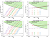Fig. 1. Particle growth tracks for a range of particle sizes St ∈ [0.01, 0.04] in four scenarios: fragmentation-limited vs. drift-limited growth, and α = 10−4 or 10−3. The particle tracks begin at the solid circle, which marks the midplane dust-to-gas ratio for vertical sedimentation in the presence of mass loading (Eq. (19)). For reference, we also show an open circle for $ϵ=Z\sqrt{\mathrm{St}/\alpha }$, which does not account for mass loading. The highlighted region is the range of midplane-averaged ϵ and St values where SI filaments cross the Hill density and are likely to experience gravitational collapse. We fine-tuned Z so that the particle tracks would converge at around two times the SI criterion (dashed line).

For each particle track we show the following:

• An open circle denoting the classic $ϵ=Z\sqrt{\mathrm{St}/\alpha }$ for the midplane dust-to-gas ratio due to sedimentation.

• A closed circle denoting the midplane dust-to-gas ratio when accounting for mass loading (Eq. (19)). This is the starting point of the particle track.

• The particle track itself, along with a label recording the initial (Z, St) for that particle track.

We find that in every single case, the combination of the SI and coagulation can lead to a drastic increase in particle size. The exact behavior depends primarily on whether the grain sizes are limited by fragmentation or radial drift.

3.1. Fragmentation limit

The SI and coagulation act together to cause a drastic increase in both St and ϵ. By trial and error we chose the smallest Z that allows each particle track to converge at around 2× the SI criterion. We find that these Z values are quite robust because very small increases in Z lead to much longer tracks. Had we chosen to stop at 1× or 3× the SI criterion, the reported Z values would have been within 2% of those reported here.

We find that as long as ϵ starts at ≥0.3, the particle track will go well inside the planetesimal-formation region. If we insert the ϵ > 0.3 criterion into Eq. (19), we obtain

$$\begin{array}{c}\hfill Z>0.0263\sqrt{{\left(\frac{\mathrm{\Pi }}{0.05}\right)}^2+\frac{\alpha /{10}^{-4}}{\alpha /{10}^{-4}+\mathrm{St}/0.01}}.\end{array}$$(21)

We note that two of the tracks in Fig. 1 start with Z = 0.0137 and Z = 0.0118, which lie just below the Z ≥ 0.015 parameter range where Eq. (2) was obtained. The most conservative choice would be to fix Z ≡ 0.015, which would bring ϵ_init to 0.29 and 0.34, respectively. Aside from these, all tracks in Fig. 1 are within the parameter range of Lim et al. (2024a)’s study.

3.2. Drift limit

This case is more subtle. The growth tracks for both barriers exhibit a kink. Initially, the growth is mainly in St with little change in ϵ. At some point, the SI becomes more effective and St and ϵ start to grow together. For the fragmentation barrier the kink appears quickly, but for the radial drift barrier the kink occurs so late that it is outside the plotted region for all examples except those that start with St = 0.01. However, if our semi-analytical fit for SI clumping extends beyond St = 0.1, that kink could still increase ϵ in the drift-dominated disk.

4. Discussion

The origin of planetesimals is a decades-old problem in planet formation. Crossing the vast chasm between millimeter- to centimeter-sized grains and 100 km planetesimals is by far the largest step needed to form a planet.

We have discovered a powerful feedback loop in which the SI and fragmentation-limited dust coagulation assist each other to accomplish something that neither one seems able to do alone: form planetesimals under typical disk conditions. That said, it is important to ponder what happens when dust sizes are not limited by fragmentation.

4.1. Drift barrier

In drift-limited regions there is also a feedback loop that can significantly increase St. However, this is not accompanied by much dust concentration, and seems to require an implausible value for Z. We speculate that planet formation in these regions requires dust traps to limit or halt radial drift.

We also note that in the drift-limited regime the growth tracks are mainly in the direction of increasing St, which reflects the shortening of the growth timescale. Therefore, at some point, the system would evolve into the fragmentation-limited regime.

4.2. Bouncing barrier

Another possibly critical barrier may occur when grain collisions simply do not result in sticking (Zsom et al. 2010). This barrier is less understood since it depends on grain properties such as shape and porosity. If present, it could drastically alter the grain size distribution (Dominik & Dullemond 2024) and lead to grains far smaller than St_frag, or it might simply be overcome by electrostatic charges (Jungmann & Wurm 2021).

With this in mind, it is worth mentioning that the bouncing barrier is similar to fragmentation in that it is a limit in v_coll. Therefore, if present, the bouncing barrier must experience the same feedback loop that we found for fragmentation. The growth tracks would look like those for St_frag, but probably starting at lower St and higher Z to reach the planetesimal formation region.

5. Conclusions

We have shown that there is a powerful feedback loop in which the SI and dust coagulation boost each other. Each process creates the environment that the other requires: The SI creates dust-dense regions with low turbulence and slow drift; these are the ideal conditions for dust coagulation to form larger grains that make the SI more effective. We developed the following three ingredients:

1. A semi-analytical estimate of the dust-to-gas ratio ϵ created by the SI (Eq. (2));

2. An analytical expression for St_frag that models turbulence dampening due to dust feedback (Eq. (8));

3. An analytical expression for St_drift that models the reduced radial drift due to dust feedback (Eq. (14)).

In the fragmentation-limited regime, the combination of the SI and dust growth led to a drastic increase in both St and ϵ, as the two processes fed each other. A practical rule of thumb is that a midplane dust-to-gas ratio of ϵ ≥ 0.3 is sufficient to reach the planetesimal-forming region across the full range of (St, α) that we explored. In other words, the positive feedback seems to resolve a decades-old problem in planet formation, at least in the fragmentation-limited inner disk.

In the drift-limited regime, we saw a dramatic increase in St, but it was not usually accompanied by a significant increase in ϵ, at least for St ≤ 0.1; however, if our semi-analytical fit for SI clumping extends to St > 0.1, it could still lead to significant increase in ϵ in the drift-dominated disk. All in all, planetesimal formation may not be possible in the drift-dominated portion of the disk without very high Z, and particle traps may be required to allow planet formation at wide orbital distances.

Data availability

The source code supporting this study is openly available at doi: https://doi.org/10.5281/zenodo.15191150

Acknowledgments

DC, WL, and JBS acknowledge support from NASA under Emerging Worlds through grant 80NSSC25K7414. J.L. acknowledges support from NASA under the Future Investigators in NASA Earth and Space Science and Technology grant 80NSSC22K1322. LE acknowledges the support from NASA via the Emerging Worlds program (80NSSC25K7117), as well as funding by the Institute for Advanced Computational Science Postdoctoral Fellowship.

References

Appendix A: How the SI boosts mass loading

Perhaps the best-known feature of the SI, and the reason it has garnered so much attention, is its ability to collect solid grains into dense filaments. Here we repurpose the dataset of Lim et al. (2024a), who conducted a large number of 3D simulations of the SI with external (i.e., forced) turbulence. We refer to that paper for details of their simulation setup. In brief, they conducted a systematic exploration of the SI for St ∈ [0.01, 0.1], Z ∈ [0.015, 0.4], and α ∈ [10⁻⁴, 10⁻³] where St ≡ t_stopΩ_K is the grain’s Stokes number, Z = Σ_p/Σ_g is the column dust-to-gas ratio, and α is the squared Mach number of the turbulence.

Our goal is to estimate the typical dust-to-gas ratio ϵ = ρ_p/ρ_g inside the SI particle filaments. First, we take the mean particle density along the azimuthal direction ⟨ρ_p(z = 0)⟩_y. This removes most of the stochastic noise. Let

$$\begin{array}{ccc}\hfill {\rho }_{\mathrm{g},\mathrm{mid}}& \equiv \hfill & \hfill {⟨{\rho }_{\mathrm{g}}(z=0)⟩}_{\mathit{xy}}\\ \hfill {\rho }_{\mathrm{p},\mathrm{mid}}& \equiv \hfill & \hfill {⟨{\rho }_{\mathrm{p}}(z=0)⟩}_{\mathit{xy}}\\ \hfill {\rho }_{\mathrm{p},\max }& \equiv \hfill & \hfill \max [{⟨{\rho }_{\mathrm{p}}(z=0)⟩}_y]\\ \hfill {\rho }_{\mathrm{p},\mathrm{dev}}& \equiv \hfill & \hfill {\rho }_{\mathrm{p},\max }-{\rho }_{\mathrm{p},\mathrm{mid}}\\ \hfill {ϵ}_{\mathrm{SI}}& \equiv \hfill & \hfill \frac{1}{{\rho }_{\mathrm{g},\mathrm{mid}}}({\rho }_{\mathrm{p},\mathrm{mid}}+\frac{{\rho }_{\mathrm{p},\mathrm{dev}}}{2}),\end{array}$$(A.1)

where ρ_p, dev is the density deviation due to the SI. At ^1/2-deviation, ϵ_SI sits near the middle of the range of ϵ values inside a filament. Figure A.1 shows ρ_p and ϵ_SI for six snapshots in two simulations. We have reviewed other snapshots and other simulations, and the results are similar. Qualitatively, Eq. A.5 appears to be a reliable measure of the typical ϵ inside an SI filament. Quantitatively, we found that most (55 − 80%) of the particles contained in the filament are in grid cells with ϵ > ϵ_SI. When the simulation first reaches a saturated state (meaning that H_p stabilizes), around 55 − 70% of the particle mass is above ϵ_SI, and that value increases to 70 − 80% before the filament reaches the Hill density. That makes ϵ_SI a conservative measure of the density environment experienced by particles inside the filament, and a good choice for exploring dust coagulation inside SI filaments.

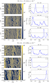Fig. A.1. Six sample snapshots from two simulations by Lim et al. (2024a), showing the midplane particle density (ρp(z = 0), left), and the midplane particle density averaged along the azimuthal direction (⟨ρp(z = 0)⟩y, right). The value of ϵSI is also shown.

For each simulation in Lim et al. (2024a) we computed ϵ_SI from the moment when ϵ_SI appears to have reached a saturated state, to the moment when ρ_p crosses the Hill density. In other words, examine the saturated state prior to gravitational collapse. We compute the time-average ⟨ϵ_SI⟩_t and standard deviation σ_ϵSI. Figure A.2 shows the time series for a sample run, and ⟨ρ_p(z = 0)⟩_y. It also shows the time-averaging interval.

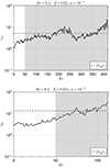Fig. A.2. Time series of ϵSI for two sample runs. The gray region shows the time interval between the moment that the simulation reaches a saturated state, until the moment when ρp crosses the Hill density (and self-gravity starts to dominate). For each simulation we compute the time average ⟨ϵSI⟩t over this interval.

To fit a semi-analytical formula for ϵ_SI, we looked for a power law of the form ϵ_SI ∝ Z^aSt^bα^c. Writing log ϵ_SI = C + alog Z + blogSt + clog α, we used ordinary least squares to find the fit:

$$\begin{array}{c}\hfill {ϵ}_{\mathrm{SI}}\approx 1.12{\left(\frac{Z}{0.01}\right)}^{2.65}{\left(\frac{\mathrm{St}}{0.1}\right)}^{1.42}{\left(\frac{\alpha }{{10}^{-4}}\right)}^{-1.38}.\end{array}$$(A.2)

SI filaments exhibit a significantly steeper dependence on all three parameters (Z, St, α) than the familiar $ϵ=Z\sqrt{\mathrm{St}/\alpha }$ for dust sedimentation.

Figure A.3 shows the ratio of ϵ_SI from our data, and the best fit in Eq. A.6. A perfect fit would have ϵ_data/ϵ_fit = 1. Notice after applying our fit, there is a slight trend where ϵ_data/ϵ_fit versus St increases slope with α while ϵ_data/ϵ_fit versus Z decreases slope with α. These trends can be removed if we modify the exponents on Z and St to include components ∝log(α). However, we judged that the increase in complexity did not justify the small improvement in the fit. For the rest of this work we use Eq. 2. Lastly, the error bars in Fig. A.3 are equal to σ_ϵSI/⟨ϵ_SI⟩_t.

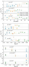Fig. A.3. Our {⟨ϵSI⟩t} dataset divided across α (top to bottom) and across Z (see inset for color-coding). We plot the ratio (ϵdata/ϵfit) of the dataset vs the fit in Eq. 2. A perfect fit would mean ϵdata/ϵfit = 1. The error bars are σϵdata/ϵdata, where σϵdata is the standard deviation of the time series.

All Figures

Fig. 1. Particle growth tracks for a range of particle sizes St ∈ [0.01, 0.04] in four scenarios: fragmentation-limited vs. drift-limited growth, and α = 10−4 or 10−3. The particle tracks begin at the solid circle, which marks the midplane dust-to-gas ratio for vertical sedimentation in the presence of mass loading (Eq. (19)). For reference, we also show an open circle for $ϵ=Z\sqrt{\mathrm{St}/\alpha }$, which does not account for mass loading. The highlighted region is the range of midplane-averaged ϵ and St values where SI filaments cross the Hill density and are likely to experience gravitational collapse. We fine-tuned Z so that the particle tracks would converge at around two times the SI criterion (dashed line).

In the text

	Fig. A.1. Six sample snapshots from two simulations by Lim et al. (2024a), showing the midplane particle density (ρp(z = 0), left), and the midplane particle density averaged along the azimuthal direction (⟨ρp(z = 0)⟩y, right). The value of ϵSI is also shown.
In the text

	Fig. A.2. Time series of ϵSI for two sample runs. The gray region shows the time interval between the moment that the simulation reaches a saturated state, until the moment when ρp crosses the Hill density (and self-gravity starts to dominate). For each simulation we compute the time average ⟨ϵSI⟩t over this interval.
In the text

	Fig. A.3. Our {⟨ϵSI⟩t} dataset divided across α (top to bottom) and across Z (see inset for color-coding). We plot the ratio (ϵdata/ϵfit) of the dataset vs the fit in Eq. 2. A perfect fit would mean ϵdata/ϵfit = 1. The error bars are σϵdata/ϵdata, where σϵdata is the standard deviation of the time series.
In the text

References

- Birnstiel, T., Dullemond, C. P., & Brauer, F. 2010, A&A, 513, A79 [NASA ADS] [CrossRef] [EDP Sciences] [Google Scholar]
- Birnstiel, T., Klahr, H., & Ercolano, B. 2012, A&A, 539, A148 [NASA ADS] [CrossRef] [EDP Sciences] [Google Scholar]
- Cañas, M. H., Lyra, W., Carrera, D., et al. 2024, PSJ, 5, 55 [Google Scholar]
- Carrera, D., Johansen, A., & Davies, M. B. 2015, A&A, 579, A43 [NASA ADS] [CrossRef] [EDP Sciences] [Google Scholar]
- Chang, P., & Oishi, J. S. 2010, ApJ, 721, 1593 [NASA ADS] [CrossRef] [Google Scholar]
- Chen, J.-W., & Lin, M.-K. 2018, MNRAS, 478, 2737 [NASA ADS] [CrossRef] [Google Scholar]
- Cuzzi, J. N., Dobrovolskis, A. R., & Champney, J. M. 1993, Icarus, 106, 102 [NASA ADS] [CrossRef] [Google Scholar]
- Dominik, C., & Dullemond, C. P. 2024, A&A, 682, A144 [NASA ADS] [CrossRef] [EDP Sciences] [Google Scholar]
- Fraser, W. C., Bannister, M. T., Pike, R. E., et al. 2017, Nat. Astron., 1, 0088 [Google Scholar]
- Güttler, C., Blum, J., Zsom, A., Ormel, C. W., & Dullemond, C. P. 2010, A&A, 513, A56 [Google Scholar]
- Ho, K. W., Li, H., & Li, S. 2024, ApJ, 975, L34 [Google Scholar]
- Johansen, A., & Youdin, A. 2007, ApJ, 662, 627 [Google Scholar]
- Johansen, A., Youdin, A., & Mac Low, M.-M. 2009, ApJ, 704, L75 [NASA ADS] [CrossRef] [Google Scholar]
- Jungmann, F., & Wurm, G. 2021, A&A, 650, A77 [NASA ADS] [CrossRef] [EDP Sciences] [Google Scholar]
- Kokubo, E., & Ida, S. 1996, Icarus, 123, 180 [Google Scholar]
- Kokubo, E., & Ida, S. 2000, Icarus, 143, 15 [Google Scholar]
- Laibe, G., & Price, D. J. 2014, MNRAS, 440, 2136 [Google Scholar]
- Li, R., & Youdin, A. N. 2021, ApJ, 919, 107 [NASA ADS] [CrossRef] [Google Scholar]
- Lim, J., Simon, J. B., Li, R., et al. 2024a, ApJ, 969, 130 [NASA ADS] [CrossRef] [Google Scholar]
- Lim, J., Simon, J. B., Li, R., et al. 2024b, arXiv e-prints [arXiv:2410.17319] [Google Scholar]
- Lin, M.-K., & Youdin, A. N. 2017, ApJ, 849, 129 [NASA ADS] [CrossRef] [Google Scholar]
- Morbidelli, A., Bottke, W. F., Nesvorný, D., & Levison, H. F. 2009, Icarus, 204, 558 [Google Scholar]
- Nakagawa, Y., Sekiya, M., & Hayashi, C. 1986, Icarus, 67, 375 [Google Scholar]
- Nesvorný, D., Youdin, A. N., & Richardson, D. C. 2010, AJ, 140, 785 [Google Scholar]
- Nesvorný, D., Li, R., Youdin, A. N., Simon, J. B., & Grundy, W. M. 2019, Nat. Astron., 3, 808 [CrossRef] [Google Scholar]
- Ormel, C. W., & Cuzzi, J. N. 2007, A&A, 466, 413 [NASA ADS] [CrossRef] [EDP Sciences] [Google Scholar]
- Schräpler, R., & Henning, T. 2004, ApJ, 614, 960 [CrossRef] [Google Scholar]
- Shi, J.-M., & Chiang, E. 2013, ApJ, 764, 20 [NASA ADS] [CrossRef] [Google Scholar]
- Tominaga, R. T., & Tanaka, H. 2023, ApJ, 958, 168 [Google Scholar]
- Voelk, H. J., Jones, F. C., Morfill, G. E., & Roeser, S. 1980, A&A, 85, 316 [Google Scholar]
- Yang, C.-C., & Zhu, Z. 2020, MNRAS, 491, 4702 [NASA ADS] [CrossRef] [Google Scholar]
- Yang, C.-C., Johansen, A., & Carrera, D. 2017, A&A, 606, A80 [NASA ADS] [CrossRef] [EDP Sciences] [Google Scholar]
- Youdin, A. N., & Goodman, J. 2005, ApJ, 620, 459 [Google Scholar]
- Youdin, A., & Johansen, A. 2007, ApJ, 662, 613 [Google Scholar]
- Youdin, A. N., & Lithwick, Y. 2007, Icarus, 192, 588 [NASA ADS] [CrossRef] [Google Scholar]
- Zsom, A., Ormel, C. W., Güttler, C., Blum, J., & Dullemond, C. P. 2010, A&A, 513, A57 [NASA ADS] [CrossRef] [EDP Sciences] [Google Scholar]