© The Authors 2025

1 Introduction

Astrophysical fluids are often a mixture of gas and solid particles or dust, at a canonical dust-to-gas ratio of 1% (see e.g. Draine et al. 2007). Since different forces act on gas and dust (e.g. gas pressure only on gas, radiation pressure only on dust), the two components often have different equilibrium velocities. In many cases, such a situation where gas and dust drift relatively to each other is hydrodynamically unstable. A wide class of such instabilities are the so-called resonant drag instabilities (RDIs; see Squire & Hopkins 2018a,b).

In the analysis of RDIs, the dust-to-gas ratio μ is taken to be a small parameter. In the absence of dust, the gas can sustain a set of waves, depending on the relevant physics (e.g. sound waves, buoyancy waves, magnetosonic waves, etc). If the gas wave speed matches the drift speed of the dust, the dust induces a particularly strong reaction to the system, often resulting in exponentially growing perturbations (Squire & Hopkins 2018b). Matching the wave and drift speeds only happens at a specific wavelength (if the wave speed depends on wavelength) and dust size (if drift speed depends on size), hence the resonant nature of the instabilities.

One can classify RDIs according to the associated gas wave. In a companion paper (Paardekooper & Aly 2025, hereafter Paper I), we studied the acoustic drag instability, which relies on a gas sound wave going unstable due to dust loading. If the gas is magnetised or stably stratified, different waves are available to create an RDI (Squire & Hopkins 2018b; Hopkins et al. 2020). In this paper, we focus on two related instabilities that are relevant for the formation of planets, as they can occur in protoplanetary discs. They are the streaming instability (SI; Youdin & Goodman 2005) and the dust settling instability (DSI; Squire & Hopkins 2018b; Krapp et al. 2020). In both cases, the underlying gas wave is an inertial wave (Zhuravlev 2019).

The SI has found its way into planet formation theory because it can potentially solve the problem of the formation of planetesimals by creating overdense dust clumps that collapse under their own gravity (for a recent review, see Lesur et al. 2023). This has always been a problematic part of planet formation theory, because rapid inward dust drift threatens to move all planetary building blocks into the central star (e.g. Weidenschilling 1977). The SI is an elegant solution to this problem, as it actually uses the drift to trigger the RDI and build bodies large enough (i.e. kilometre-sized planetesimals) on a short enough timescale to be safe from drifting too far in.

Since dust drift usually depends on dust size, because smaller particles are more tightly coupled to the gas, extending the RDI formalism to incorporate a distribution of dust sizes is not straightforward. For a given gas wave, only a single particle size will drift at the resonant speed, but if the other sizes are passive one might hope that the feedback loop leading to the RDI (see Magnan et al. 2024a) can survive. Indeed, some simulations indicate that the clumping induced by the SI is not very sensitive to having a size distribution (Schaffer et al. 2021; Rucska & Wadsley 2023). However, this turns out not to be true for the linear phase, at least in the case where vertical stratification is neglected (as was done in the original work of Youdin & Goodman 2005).

The effect of a dust size distribution on the linear SI was investigated by Krapp et al. (2019), who found that for a discrete number of different particle sizes, in many regions of parameter space the growth rate of the SI keeps decreasing with the number of particle sizes considered. It was shown in Paardekooper et al. (2020) that in the limit of a continuous size distribution, the SI indeed ceases to exist except at extremely small wavelengths at dust-to-gas ratios much higher than unity (see also Zhu & Yang 2021). These small scales are particularly prone to viscous damping, so in addition a top-heavy size distribution is needed for the linear SI to survive (McNally et al. 2021).

The non-linear evolution of the SI with multiple dust sizes was studied in Yang & Zhu (2021), which found that one either needs a dust-to-gas ratio μ > 1 or a maximum stopping time τ_s > 1 to achieve significant activity in the non-linear regime. It should be noted again that these results, as in the original SI analysis (Youdin & Goodman 2005), neglect vertical stratification in the disc and that the SI may well have a different character in the stratified case (Lin 2021); and it could react differently to a size distribution, at least in the non-linear regime (see e.g. Schaffer et al. 2021; Rucska & Wadsley 2023).

The settling instability is a more recently discovered RDI that is also reliant on inertial waves but takes into account vertical dust drift such as settling (Squire & Hopkins 2018b). In Krapp et al. (2020), it was reported that this RDI is far less sensitive to a size distribution and is able to maintain strong growth rates even for wide size distributions. This raises a question as to which RDIs can survive in the presence of a dust size distribution and therefore contribute to, for example, planetesimal formation (e.g. Johansen et al. 2007). In a companion paper, we showed that a polydisperse version of the acoustic drag instability exists, but only for large wavelengths, which reduces the maximum growth rate significantly. In this paper, we focus on polydisperse versions of both the streaming and settling instability, in the regime where μ ≪ 1 to make contact with monodisperse RDI results. We focus on whether these exist in a polydisperse context, and, if so, how the growth rates compare to the monodisperse case.

The plan of this paper is as follows. We introduce the basic equations in Sect. 2. We present the results on the streaming and settling instability in Sects. 3 and 4, respectively, and we conclude in Sect. 5.

2 Governing equations

The equations governing a mixture of gas and dust, where the dust component consists of a continuum of sizes, were presented in Paardekooper et al. (2021) (see also Paper I): $${\partial }_t\sigma +\nabla \cdot (\sigma \mathbf{u})=0,$$(1) $${\partial }_t\mathbf{u}+(\mathbf{u}\cdot \nabla )\mathbf{u}={\mathbf{\alpha }}_{\mathrm{d}}-\frac{\mathbf{u}-{\mathbf{v}}_{\mathrm{g}}}{{\tau }_{\mathrm{s}}},$$(2) with u being the size-dependent dust velocity, and v_g the gas velocity. The quantity σ is the size density (Paardekooper et al. 2020), defined such that $${\rho }_{\mathrm{d}}={\displaystyle \int }\sigma \mathrm{d}{\tau }_{\mathrm{s}},$$(3) with ρ_d being the dust density and τ_s the stopping time, which is a proxy for particle size. As in Paper I, we took the simplest drag law of the form (u v_g)/τ_s to couple gas and dust, with constant stopping time τ_s. Any additional accelerations acting on the dust are contained in α_d, which we assume to depend on u only. The gas component, similarly, has its continuity and momentum equation, where the back-reaction of drag on the gas enters the latter as an integral over stopping time: $${\partial }_t{\rho }_{\mathrm{g}}+\nabla \cdot ({\rho }_{\mathrm{g}}{\mathbf{v}}_{\mathrm{g}})=0,$$(4) $${\partial }_t{\mathbf{v}}_{\mathrm{g}}+({\mathbf{v}}_{\mathrm{g}}\cdot \nabla ){\mathbf{v}}_{\mathrm{g}}=-\frac{\nabla p}{{\rho }_{\mathrm{g}}}+{\mathbf{\alpha }}_{\mathrm{g}}+\frac{1}{{\rho }_{\mathrm{g}}}\int \sigma \frac{\mathbf{u}-{\mathbf{v}}_{\mathrm{g}}}{{\tau }_{\mathrm{s}}}\mathrm{d}{\tau }_{\mathrm{s}},$$(5) where ρ_g is the gas density, p the pressure, and all additional accelerations on the gas are contained in α_g.

Our basic setup is a standard unstratified shearing box (Goldreich & Lynden-Bell 1965; Hawley et al. 1995; Latter & Papaloizou 2017). Following Krapp et al. (2020), to account for vertical stratification, we added an extra vertical acceleration to the dust component ${\alpha }_{\text{d}}=z_0{\mathrm{\Omega }}^2\widehat{z}$, where z₀ can be thought of as the height of the box above the mid plane¹. For the gas, this vertical acceleration is balanced by a background pressure gradient, which we subtracted from the total pressure. What is left is the back-reaction on the gas, μz₀Ω², whereby the total acceleration of gas and dust are given by $${\mathbf{\alpha }}_{\mathrm{g}}=2\eta \widehat{\mathbf{x}}-\mu z_0{\mathrm{\Omega }}^2\widehat{\mathbf{z}}-2\mathbf{\Omega }\times {\mathbf{v}}_{\mathrm{g}}-\nabla \mathrm{\Phi },$$(6) $${\mathbf{\alpha }}_{\mathrm{d}}=z_0{\mathrm{\Omega }}^2\widehat{\mathbf{z}}-2\mathbf{\Omega }\times \mathbf{u}-\nabla \mathrm{\Phi },$$(7)

The potential Φ = SΩx², where S is the rate of orbital shear. The parameter η is determined by the global radial pressure gradient, η = 1/(2ρ_g)dP/dr (Paardekooper et al. 2020). The equations governing the gas are then given by Eqs. (4) and (5), with accelerations as stated above (for a more formal derivation, see Appendix A): $${\partial }_t{\rho }_{\mathrm{g}}+\nabla \cdot ({\rho }_{\mathrm{g}}{\mathbf{v}}_{\mathrm{g}})=0,$$(8) $$\begin{array}{l}{\partial }_t{\mathbf{v}}_{\mathrm{g}}+({\mathbf{v}}_{\mathrm{g}}\cdot \nabla ){\mathbf{v}}_{\mathrm{g}}=2\eta \widehat{\mathbf{x}}-\mu z_0{\mathrm{\Omega }}^2\widehat{\mathbf{z}}-\frac{\nabla p}{{\rho }_{\mathrm{g}}}-2\mathbf{\Omega }\times {\mathbf{v}}_{\mathrm{g}}-\nabla \mathrm{\Phi }\\ \hfill +\frac{1}{{\rho }_{\mathrm{g}}}\int \sigma \frac{\mathbf{u}-{\mathbf{v}}_{\mathrm{g}}}{{\tau }_{\mathrm{s}}}\mathrm{d}{\tau }_{\mathrm{s}}.\hfill \end{array}$$(9)

It should be noted that the pressure does not include the vertical stratification; stratification is only taken into account through the accelerations involving z₀Ω². We took the equation of state to be isothermal, p = c²ρ_g, with the constant sound speed being c. We fixed c by requiring that η/(cΩ) = 10^−3/2, similar to the choice in Krapp et al. (2020)². The dust fluid equations can similarly be constructed from Eqs. (1) and (2): $${\partial }_t\sigma +\nabla \cdot (\sigma \mathbf{u})=0,$$(10) $${\partial }_t\mathbf{u}+(\mathbf{u}\cdot \nabla )\mathbf{u}=z_0{\mathrm{\Omega }}^2\widehat{\mathbf{z}}-2\mathbf{\Omega }\times \mathbf{u}-\nabla \mathrm{\Phi }-\frac{\mathbf{u}-{\mathbf{v}}_{\mathrm{g}}}{{\tau }_{\mathrm{s}}}.$$(11)

Apart from the extra vertical acceleration, these equations are the same as in Paardekooper et al. (2020) and Paardekooper et al. (2021). With these shearing-box equations for the gas-dust system in hand, we can proceed to solving for the equilibrium state.

2.1 Equilibrium state

For the equilibrium state, we took ρ_g and σ to be spatially constant. An equilibrium solution can then be found with horizontal velocities independent of y and z (Paardekooper et al. 2020): $$v_{\mathrm{g}x}=\frac{2\eta }{\kappa }\frac{{\mathcal{J}}_1}{{(1+{\mathcal{J}}_0)}^2+{\mathcal{J}}_1^2},$$(12) $$v_{\mathrm{g}y}=-Sx-\frac{\eta }{\mathrm{\Omega }}\frac{1+{\mathcal{J}}_0}{{(1+{\mathcal{J}}_0)}^2+{\mathcal{J}}_1^2},$$(13) $$u_x=\frac{2\eta }{\kappa }\frac{{\mathcal{J}}_1-\kappa {\tau }_{\mathrm{s}}(1+{\mathcal{J}}_0)}{(1+{\kappa }^2{\tau }_{\mathrm{s}}^2)({(1+{\mathcal{J}}_0)}^2+{\mathcal{J}}_1^2)},$$(14) $$u_y=-Sx-\frac{\eta }{\mathrm{\Omega }}\frac{1+{\mathcal{J}}_0+\kappa {\tau }_{\mathrm{s}}{\mathcal{J}}_1}{(1+{\kappa }^2{\tau }_{\mathrm{s}}^2)({(1+{\mathcal{J}}_0)}^2+{\mathcal{J}}_1^2)},$$(15) with integrals $${\mathcal{J}}_m=\frac{1}{{\rho }_{\mathrm{g}}}\int \frac{\sigma {(\kappa {\tau }_{\mathrm{s}})}^m}{1+{\kappa }^2{\tau }_{\mathrm{s}}^2}\mathrm{d}{\tau }_{\mathrm{s}}.$$(16)

Here, κ² = 2Ω(S − Ω) is the square of the epicyclic frequency, with shear rate S . In a Keplerian disc, S = 3Ω/2, in which case κ = Ω. Vertical dust velocities are constant in space and given by $$u_z={\tau }_{\mathrm{s}}{z}_0{\mathrm{\Omega }}^2,$$(17) while the vertical gas velocity is zero. The dust velocities correspond to a uniform vertical settling flow for each dust size at the appropriate terminal velocity in the uniform vertical gravitational field of the model.

2.2 Linear perturbations

We considered small perturbations ${\rho }_{\text{g}}={\rho }_{\text{g}}^{(0)}+{\rho }_{\text{g}}^{(1)}$ with ${\rho }_{\text{g}}^{(1)}\ll {\rho }_{\text{g}}^{(0)}$, and we adopted a similar form for other quantities. Ignoring quadratic terms in perturbed quantities, we find the following from the gas equations: $${\partial }_t{\rho }_{\mathrm{g}}^{(1)}+{\mathbf{v}}_{\mathrm{g}}^{(0)}\cdot \nabla {\rho }_{\mathrm{g}}^{(1)}+{\rho }_{\mathrm{g}}^{(0)}\nabla \cdot {\mathbf{v}}_{\mathrm{g}}^{(1)}=0,$$(18) $$\begin{array}{l}{\partial }_t{\mathbf{v}}_{\mathrm{g}}^{(1)}+({\mathbf{v}}_{\mathrm{g}}^{(0)}\cdot \nabla ){\mathbf{v}}_{\mathrm{g}}^{(1)}-S{v}_{\mathrm{g}x}^{(1)}\widehat{\mathbf{y}}=-\frac{\nabla p^{(1)}}{{\rho }_{\mathrm{g}}^{(0)}}-2\mathbf{\Omega }\times {\mathbf{v}}_{\mathrm{g}}^{(1)}\\ +\frac{1}{{\rho }_{\mathrm{g}}^{(0)}}\int {\sigma }^{(1)}\frac{\mathrm{\Delta }{\mathbf{u}}^{(0)}}{{\tau }_{\mathrm{s}}}\mathrm{d}{\tau }_{\mathrm{s}}+\frac{1}{{\rho }_{\mathrm{g}}^{(0)}}\int {\sigma }^{(0)}\frac{{\mathbf{u}}^{(1)}-{\mathbf{v}}_{\mathrm{g}}^{(1)}}{{\tau }_{\mathrm{s}}}\mathrm{d}{\tau }_{\mathrm{s}}.\end{array}$$(19) with equilibrium relative velocity $\mathrm{\Delta }{u}^{(0)}=u^{(0)}-v_{\text{g}}^{(0)}$. Dust perturbations are governed by $${\partial }_t{\sigma }^{(1)}+{\mathbf{u}}^{(0)}\cdot \nabla {\sigma }^{(1)}+{\sigma }^{(0)}\nabla \cdot {\mathbf{u}}^{(1)}=0,$$(20) $$\begin{array}{l}{\partial }_t{\mathbf{u}}^{(1)}+({\mathbf{u}}^{(0)}\cdot \nabla ){\mathbf{u}}^{(1)}-S{u}_x^{(1)}\widehat{\mathbf{y}}=-2\mathbf{\Omega }\times {\mathbf{u}}^{(1)}-\frac{{\mathbf{u}}^{(1)}-{\mathbf{v}}_{\mathrm{g}}^{(1)}}{{\tau }_{\mathrm{s}}}\\ -\frac{{\rho }_{\mathrm{g}}^{(1)}}{{\rho }_{\mathrm{g}}^{(0)}}\frac{\mathrm{\Delta }{\mathbf{u}}^{(0)}}{{\tau }_{\mathrm{s}}}.\end{array}$$(21)

We consider perturbations of the form $X^{(1)}(x,t,\tau )=\widehat{X}(\tau )\text{exp}(ik\cdot x-i\omega t)$, with wave number k = (k_x, k_y, k_z)^T and frequency ω. We only consider perturbations with k_y = 0. Using the above form of the perturbations, the dust and gas perturbation equations transform to $$k_x{v}_{\mathrm{g}x}^{(0)}\frac{{\widehat{\rho }}_{\mathrm{g}}}{{\rho }_{\mathrm{g}}^{(0)}}+\mathbf{k}\cdot {\widehat{\mathbf{v}}}_{\mathrm{g}}=\omega \frac{{\widehat{\rho }}_{\mathrm{g}}}{{\rho }_{\mathrm{g}}^{(0)}},$$(22) $$k_x{v}_{\mathrm{g}x}^{(0)}{\widehat{\mathbf{v}}}_{\mathrm{g}}+\mathrm{i}S{\widehat{v}}_{\mathrm{g}x}\widehat{\mathbf{y}}+\frac{\mathbf{k}{c}^2{\widehat{\rho }}_{\mathrm{g}}}{{\rho }_{\mathrm{g}}^{(0)}}-2\mathrm{i}\mathbf{\Omega }\times {\widehat{\mathbf{v}}}_{\mathrm{g}}+\widehat{\mathbf{b}}=\omega {\widehat{\mathbf{v}}}_{\mathrm{g}},$$(23) $$\mathbf{k}\cdot {\mathbf{u}}^{(0)}\widehat{\sigma }+{\sigma }^{(0)}\mathbf{k}\cdot \widehat{\mathbf{u}}=\omega \widehat{\sigma },$$(24) $$\begin{array}{l}(\mathbf{k}\cdot {\mathbf{u}}^{(0)})\widehat{\mathbf{u}}+\mathrm{i}S{\widehat{u}}_x\widehat{\mathbf{y}}-2\mathrm{i}\mathbf{\Omega }\times \widehat{\mathbf{u}}\\ -\mathrm{i}\frac{\widehat{\mathbf{u}}-{\widehat{\mathbf{v}}}_{\mathrm{g}}}{{\tau }_{\mathrm{s}}}-\mathrm{i}\frac{{\widehat{\rho }}_{\mathrm{g}}}{{\rho }_{\mathrm{g}}^{(0)}}\frac{\mathrm{\Delta }{\mathbf{u}}^{(0)}}{{\tau }_{\mathrm{s}}}=\omega \widehat{\mathbf{u}},\end{array}$$(25) with the back-reaction integral $$\widehat{\mathbf{b}}=\frac{\mathrm{i}}{{\rho }_{\mathrm{g}}^{(0)}}\int \frac{{\sigma }^{(0)}}{{\tau }_{\mathrm{s}}}\left[\frac{\widehat{\sigma }}{{\sigma }^{(0)}}\mathrm{\Delta }{\mathbf{u}}^{(0)}+\widehat{\mathbf{u}}-{\widehat{\mathbf{v}}}_{\mathrm{g}}\right]\mathrm{d}{\tau }_{\mathrm{s}}.$$(26)

By taking the complex conjugate of each term in Eqs. (22)–(25), it is straightforward to see that a solution with an eigenvalue ω and eigenvector ($({\widehat{\rho }}_{\text{g}},{\widehat{v}}_{\text{g}},\widehat{\sigma },\widehat{u})$ can be transformed into a solution with the eigenvalue −ω* and eigenvector $({\widehat{\rho }}_{\text{g}}^{\ast },{\widehat{v}}_{\text{g}}^{\ast },{\widehat{\sigma }}^{\ast },{\widehat{u}}^{\ast })$, where an asterisk denotes complex conjugate. Since ω and −ω^* have the same imaginary part and therefore growth rate, we follow the convention of for example Youdin & Goodman (2005); Squire & Hopkins (2018b); Krapp et al. (2019) and focus exclusively on k_x, k_z > 0.

With the help of the dust continuity and momentum equations (see Appendix B), the back-reaction integral can be written as $$\widehat{\mathbf{b}}=\mathsf{M}{\widehat{\mathbf{v}}}_{\mathrm{g}},$$(27) with the matrix M defined in Eq. (B.11). In the limit of μ ≪ 1, we therefore have a perturbed eigenvalue problem for the gas: $$\begin{array}{l}\hfill {\displaystyle (}\begin{array}{llll}\hfill k_x{v}_{\mathrm{g},x}^{(0)}\hfill & \hfill k_x\hfill & \hfill 0\hfill & \hfill k_z\hfill \\ \hfill k_x{c}^2\hfill & \hfill k_x{v}_{\mathrm{g},x}^{(0)}\hfill & \hfill 2\mathrm{i}\mathrm{\Omega }\hfill & \hfill 0\hfill \\ \hfill 0\hfill & \hfill (S-2\mathrm{\Omega })\mathrm{i}\hfill & \hfill k_x{v}_{\mathrm{g},x}^{(0)}\hfill & \hfill 0\hfill \\ \hfill k_z{c}^2\hfill & \hfill 0\hfill & \hfill 0\hfill & \hfill k_x{v}_{\mathrm{g},x}^{(0)}\hfill \end{array}\left){\displaystyle (}\begin{array}{c}\hfill {\widehat{\rho }}_{\mathrm{g}}/{\rho }_{\mathrm{g}}^{(0)}\hfill \\ \hfill {\widehat{\mathbf{v}}}_{\mathrm{g}}\hfill \end{array}\right)\hfill \\ \hfill +{\displaystyle (}\begin{array}{cc}\hfill 0\hfill & \hfill 0\hfill \\ \hfill 0\hfill & \hfill \mathsf{M}\hfill \end{array}\left)\right(\begin{array}{c}\hfill {\widehat{\rho }}_{\mathrm{g}}/{\rho }_{\mathrm{g}}^{\left(0\right)}\hfill \\ \hfill {\widehat{\mathbf{v}}}_{\mathrm{g}}\hfill \end{array})=\omega (\begin{array}{c}\hfill {\widehat{\rho }}_{\mathrm{g}}/{\rho }_{\mathrm{g}}^{\left(0\right)}\hfill \\ \hfill {\widehat{\mathbf{v}}}_{\mathrm{g}}\hfill \end{array}),\hfill \end{array}$$(28) where the perturbation matrix contains the back-reaction on the gas and is therefore ∝ μ. In regions of parameter space where the resonance is not important, ordinary eigenvalue perturbation theory can be used to approximate the growth rates for μ ≪ 1. Numerical results on growth rates were obtained by the package PSITOOLS (Paardekooper et al. 2021).

It is often useful to define a length scale η/Ω² and a time scale Ω⁻¹ and work with dimensionless wave numbers K = kη/Ω² and dimensionless stopping time, or Stokes number, St = Ωτ_s. It is worth noting that the non-dimensional ‘height’ above the midplane, ${\tilde{z}}_0=z_0{\mathrm{\Omega }}^2/\eta ,$ is a large number if we take z₀ ~ H, where H is the vertical scale height of the gas disc.

2.3 Eigenvalue perturbation theory for the inertial wave RDI

The perturbed eigenvalue problem for the inertial wave RDI Eq. (28) can be simplified by taking the gas to be incompressible. In this case, the gas Eqs. (22)–(23) can be simplified by taking the cross-product of the wave vector with the gas momentum equation: $$k_x{v}_{\mathrm{g}x}^{(0)}{\widehat{\mathbf{w}}}_{\mathrm{g}}+\mathrm{i}S{\widehat{v}}_{\mathrm{g}x}(\mathbf{k}\times \widehat{\mathbf{y}})-2\mathrm{i}\mathbf{k}\times (\mathbf{\Omega }\times {\widehat{\mathbf{v}}}_{\mathrm{g}})+\mathbf{k}\times \widehat{\mathbf{b}}=\omega {\widehat{\mathbf{w}}}_{\mathrm{g}},$$(29) with the vorticity perturbation ${\widehat{w}}_{\text{g}}=k\times {\widehat{v}}_{\text{g}}={(-k_z{\widehat{v}}_{\text{g}y},k_z{\widehat{v}}_{\text{g}x}-k_x{\widehat{v}}_{\text{g}z},k_x{\widehat{v}}_{\text{g}y})}^T$. We expand the components of the Coriolis terms to find $$k_x{v}_{\mathrm{g}x}^{(0)}{\widehat{\mathbf{w}}}_{\mathrm{g}}+\mathrm{i}\left(\begin{array}{c}(2\mathrm{\Omega }-S)k_z{\widehat{v}}_{\mathrm{g}x}\\ 2\mathrm{\Omega }{k}_z{\widehat{v}}_{\mathrm{g}y}\\ -(2\mathrm{\Omega }-S)k_x{\widehat{v}}_{\mathrm{g}x}\end{array}\right)+\mathbf{k}\times \widehat{\mathbf{b}}=\omega {\widehat{\mathbf{w}}}_{\mathrm{g}},$$(30)

We note that the last component of ${\widehat{w}}_{\text{g}}$ is redundant, so we only need to keep the first two components, and that ${\widehat{v}}_{\text{g}x}=k_z{w}_{\text{g}y}/(k_x^2+k_z^2)$: $$k_x{v}_{\mathrm{g}x}^{(0)}{\widehat{\mathbf{w}}}_{\mathrm{g}}+\mathrm{i}\left(\begin{array}{c}(2\mathrm{\Omega }-S){\widehat{k}}_z^2{w}_{\mathrm{g}y}\\ -2\mathrm{\Omega }{w}_{\mathrm{g}x}\end{array}\right)+\mathsf{K}\widehat{\mathbf{b}}=\omega {\widehat{\mathbf{w}}}_{\mathrm{g}},$$(31) with ${\widehat{k}}_z=k_z/\left|k\right|$ and the matrix $$\mathsf{K}=\left(\begin{array}{ccc}0& -k_z& 0\\ k_z& 0& -k_x\end{array}\right),$$(32) representing the cross-product with the wave vector. We can write Eq. (31) in simple matrix form: $$\left(\begin{array}{cc}{k}_x{v}_{\mathrm{g}x}^{(0)}& \mathrm{i}(2\mathrm{\Omega }-S){\widehat{k}}_z^2\\ -2\mathrm{i}\mathrm{\Omega }& k_x{v}_{\mathrm{g}x}^{(0)}\end{array}\right){\widehat{\mathbf{w}}}_{\mathrm{g}}+\mathsf{K}\mathsf{M}{\mathsf{K}}^{\prime }{\widehat{\mathbf{w}}}_{\mathrm{g}}=\omega {\widehat{\mathbf{w}}}_{\mathrm{g}},$$(33) with the matrix $${\mathsf{K}}^{\prime }=\left(\begin{array}{cc}0& k_z/k^2\\ -1/k_z& 0\\ 0& -k_x/k^2\end{array}\right).$$(34)

We now have a perturbed eigenvalue problem $({\mathsf{T}}_0+{\mathsf{T}}_1){\widehat{w}}_{\text{g}}=\omega {\widehat{w}}_{\text{g}}$. The unperturbed matrix T₀ gives the familiar inertial waves, advected with the background gas flow. The corresponding eigenvalues are $${\omega }_0=k_x{v}_{\mathrm{g}x}^{(0)}\pm {\widehat{k}}_z\kappa ,$$(35) and the left and right eigenvectors are $${\mathbf{e}}_L=\left(\begin{array}{c}\mp \frac{\mathrm{i}}{{\widehat{k}}_z}\\ \frac{\kappa }{2\mathrm{\Omega }}\end{array}\right),$$(36) $${\mathbf{e}}_R=\left(\begin{array}{c}\pm \mathrm{i}{\widehat{k}}_z\frac{\kappa }{2\mathrm{\Omega }}\\ 1\end{array}\right).$$(37)

The first-order correction to the eigenvalue due to T₁ is simply given by $${\omega }_1=\frac{{\mathbf{e}}_L^{*}{\mathsf{T}}_1{\mathbf{e}}_R}{{\mathbf{e}}_L^{*}{\mathbf{e}}_R},$$(38) where e_L and e_R are the left and right eigenvectors of T₀ corresponding to the unperturbed eigenvalue ω₀ given above, and * denotes complex conjugate. Together with the perturbation matrix $${\mathsf{T}}_1=\mathsf{K}\mathsf{M}{\mathsf{K}}^{\prime },$$(39) we can calculate the correction to the eigenvalues in the limit of μ ≪ 1 (as long as the perturbation is regular).

Since the eigenvalue perturbation is linear in the elements of T₁, and therefore linear in the elements of M, it is straightforward to distill the contributions of the dust density perturbation and the velocity perturbations to ω₁ (see Appendix B for the definitions of matrices D and A): $${\mathsf{M}}_{\sigma }=\int \frac{\mathrm{i}{\sigma }^{(0)}}{{\rho }_{\mathrm{g}}^{(0)}{\tau }_{\mathrm{s}}}{\mathsf{V}}_{\sigma }{\mathsf{A}}^{-1}\mathsf{D}\mathrm{d}{\tau }_{\mathrm{s}},$$(40) $${\mathsf{M}}_u=\int \frac{\mathrm{i}{\sigma }^{(0)}}{{\rho }_{\mathrm{g}}^{(0)}{\tau }_{\mathrm{s}}}{\mathsf{A}}^{-1}\mathsf{D}\mathrm{d}{\tau }_{\mathrm{s}},$$(41) $${\mathsf{M}}_v=-\int \frac{\mathrm{i}{\sigma }^{(0)}}{{\rho }_{\mathrm{g}}^{(0)}{\tau }_{\mathrm{s}}}\mathrm{d}{\tau }_{\mathrm{s}}\mathsf{I},$$(42) with $${\mathsf{V}}_{\sigma }=\frac{1}{\omega -k_x{u}_x^{(0)}-k_z{u}_z^{(0)}}\left(\begin{array}{ccc}\mathrm{\Delta }{u}_x^{(0)}{k}_x& 0& \mathrm{\Delta }{u}_x^{(0)}{k}_z\\ \mathrm{\Delta }{u}_y^{(0)}{k}_x& 0& \mathrm{\Delta }{u}_y^{(0)}{k}_z\\ \mathrm{\Delta }{u}_z^{(0)}{k}_x& 0& \mathrm{\Delta }{u}_z^{(0)}{k}_z\end{array}\right).$$(43)

If we use M_σ to calculate T₁ and ω₁, we only obtain the contribution from the dust density perturbation. It is convenient to combine the dust and gas velocity perturbations and look at the contribution of the relative velocity perturbation governed by M_u + M_v.

We can try and isolate the contribution of the resonance to the growth rate by focusing on the dust density perturbation: $${\omega }_{1,\sigma }=\frac{{\mathbf{e}}_L^{*}\mathsf{K}{\mathsf{M}}_{\sigma }{\mathsf{K}}^{\prime }{\mathbf{e}}_R}{{\mathbf{e}}_L^{*}{\mathbf{e}}_R}=\int \frac{\mathrm{i}{\sigma }^{(0)}}{{\rho }_{\mathrm{g}}^{(0)}{\tau }_{\mathrm{s}}}\frac{{\mathbf{e}}_L^{*}\mathsf{K}{\mathsf{V}}_{\sigma }{\mathsf{A}}^{-1}\mathsf{D}{\mathsf{K}}^{\prime }{\mathbf{e}}_R}{{\mathbf{e}}_L^{*}{\mathbf{e}}_R}\mathrm{d}{\tau }_{\mathrm{s}}.$$(44)

We can isolate the resonance contribution by defining matrix R such that ${\mathsf{V}}_{\sigma }=\mathsf{R}/(\omega -k_x{u}_x^{(0)}-k_z{u}_z^{(0)})$: $${\omega }_{1,\sigma }=\int \frac{g({\tau }_{\mathrm{s}})}{{\omega }_0-k_x{u}_x^{(0)}-k_z{u}_z^{(0)}}\mathrm{d}{\tau }_{\mathrm{s}},$$(45) with $$g({\tau }_{\mathrm{s}})=\frac{\mathrm{i}{\sigma }^{(0)}}{{\rho }_{\mathrm{g}}^{(0)}{\tau }_{\mathrm{s}}}\frac{{\mathbf{e}}_L^{*}\mathsf{K}\mathsf{R}{\mathsf{A}}^{-1}\mathsf{D}{\mathsf{K}}^{\prime }{\mathbf{e}}_R}{{\mathbf{e}}_L^{*}{\mathbf{e}}_R},$$(46) a complex scalar function, approximate Δu_x = −2ητ_s, and use u_z = Ω²z₀τ_s, as well as the expression (35) for ω₀: $$\frac{{\omega }_{1,\sigma }}{\mathrm{\Omega }}=\int \frac{\tilde{g}(\mathrm{S}\mathrm{t})}{\pm {\widehat{k}}_z+(2K_x-K_z{\tilde{z}}_0)\mathrm{S}\mathrm{t}}\mathrm{d}\mathrm{S}\mathrm{t},$$(47) with non-dimensional $\tilde{g}=g/{\mathrm{\Omega }}^2$. We note that, for a resonance to occur, we need $\pm {\widehat{k}}_z/(K_z{\tilde{z}}_0-2K_x)<0$. This means that, at a given Stokes number, the two branches of inertial waves give rise to resonances at different locations in K space. These two resonant branches come together at $K_z{\tilde{z}}_0=2K_x$, which is the location of the double resonance (Squire & Hopkins 2018b); we did not consider this here since ordinary perturbation theory does not hold. On the other hand, for a fixed wave vector K, if $\pm {\widehat{k}}_z/(K_z{\tilde{z}}_0-2K_x)<0$ there is a Stokes number that gives rise to a resonance, at least if it is inside the original size range.

It is convenient to substitute $\xi =(2K_x-K_z{\tilde{z}}_0)\pm {\widehat{k}}_z$, so at the resonant Stokes number St_res we have ξ = 0. If we further assume that $\tilde{g}$ can be expanded in a Taylor series around St = St_res or, equivalently, around ξ = 0, $$\tilde{g}(\mathrm{S}\mathrm{t})={\displaystyle \sum _{n=0}^{\infty }}{\tilde{g}}_n{(\mathrm{S}\mathrm{t}-\mathrm{S}{\mathrm{t}}_{\mathrm{r}\mathrm{e}\mathrm{s}})}^n={\displaystyle \sum _{n=0}^{\infty }}\frac{{\tilde{g}}_n}{{(2K_x-K_z{\tilde{z}}_0)}^n}{\xi }^n,$$(48) we obtain $$\frac{{\omega }_{1,\sigma }}{\mathrm{\Omega }}={\displaystyle \sum _{n=0}^{\infty }}\frac{{\tilde{g}}_n}{{(2K_x-K_z{\tilde{z}}_0)}^{n+1}}\int \frac{{\xi }^n}{\xi }\mathrm{d}\xi ,$$(49) where we explicitly kept the denominator in place to highlight the resonance. For n > 0, the integral is straightforward: $$\frac{{\omega }_{1,\sigma }}{\mathrm{\Omega }}=\frac{{\tilde{g}}_0}{2K_x-K_z{\tilde{z}}_0}\int \frac{\mathrm{d}\xi }{\xi }+{\displaystyle \sum _{n=1}^{\infty }}\frac{{\tilde{g}}_n}{{(2K_x-K_z{\tilde{z}}_0)}^{n+1}}\frac{{\xi }_{\mathrm{m}\mathrm{a}\mathrm{x}}^n-{\xi }_{\mathrm{m}\mathrm{i}\mathrm{n}}^n}{n}.$$(50)

We solve the remaining integral adopting the Landau prescription, which is well-known from plasma physics (Landau 1946) and also used in the theory of collisionless stellar systems (Binney & Tremaine 2008) and disc-planet interaction (Paardekooper & Papaloizou 2008). Including a small damping term -σ⁽¹⁾/t_damp on the right hand side of Eq. (20) leads to a small imaginary part iϵ = i/(Ωt_damp) in the denominator of the integrand in Eq. (50). To arrive at the relevant limit of no damping, we let ϵ → 0: $$\begin{array}{l}{\int }_{{\xi }_{\mathrm{m}\mathrm{i}\mathrm{n}}}^{{\xi }_{\mathrm{m}\mathrm{a}\mathrm{x}}}\frac{\mathrm{d}\xi }{\xi +\mathrm{i}ϵ}={\int }_{{\xi }_{\mathrm{m}\mathrm{i}\mathrm{n}}}^{{\xi }_{\mathrm{m}\mathrm{a}\mathrm{x}}}\frac{\xi -\mathrm{i}ϵ}{{\xi }^2+{ϵ}^2}\mathrm{d}\xi \\ =\left[\frac{\log ({\xi }^2+{ϵ}^2)}{2}-\mathrm{i}{\tan }^{-1}\left(\frac{\xi }{ϵ}\right)\right]{}_{{\xi }_{\mathrm{m}\mathrm{i}\mathrm{n}}}^{{\xi }_{\mathrm{m}\mathrm{a}\mathrm{x}}}.\end{array}$$(51)

We note that ξ_max corresponds to the value of ξ at St = St_max. Depending on the sign of $2K_x-K_z{\tilde{z}}_0$, ξ_max may be positive or negative. Therefore, in the limit ϵ → 0, we obtain that $${\int }_{{\xi }_{\mathrm{m}\mathrm{i}\mathrm{n}}}^{{\xi }_{\mathrm{m}\mathrm{a}\mathrm{x}}}\frac{\mathrm{d}\xi }{\xi +\mathrm{i}ϵ}=\log \left(\frac{|{\xi }_{\mathrm{m}\mathrm{a}\mathrm{x}}|}{|{\xi }_{\mathrm{m}\mathrm{i}\mathrm{n}}|}\right)-\mathrm{i}\pi \left(\frac{{\xi }_{\mathrm{m}\mathrm{a}\mathrm{x}}}{|{\xi }_{\mathrm{m}\mathrm{a}\mathrm{x}}|}-\frac{{\xi }_{\mathrm{m}\mathrm{i}\mathrm{n}}}{|{\xi }_{\mathrm{m}\mathrm{i}\mathrm{n}}|}\right),$$(52) where the last factor in parentheses makes sure that we only obtain a contribution if the resonance is in the domain, that is, when ξ_max and ξ_min have opposite sign, and that the sign is exchanged if ξ_max and ξ_min both change signs. In terms of Stokes numbers, we obtain $$\begin{array}{l}\frac{{\omega }_{1,\sigma }}{\mathrm{\Omega }}=\frac{{\tilde{g}}_0}{2K_x-K_z{\tilde{z}}_0}\log \left(\frac{|\mathrm{S}{\mathrm{t}}_{\mathrm{m}\mathrm{a}\mathrm{x}}-\mathrm{S}{\mathrm{t}}_{\mathrm{r}\mathrm{e}\mathrm{s}}|}{|\mathrm{S}{\mathrm{t}}_{\mathrm{m}\mathrm{i}\mathrm{n}}-\mathrm{S}{\mathrm{t}}_{\mathrm{r}\mathrm{e}\mathrm{s}}|}\right)\\ -\frac{{\tilde{g}}_0}{|2K_x-K_z{\tilde{z}}_0|}\frac{\mathrm{i}\pi }{2}\left[\frac{\mathrm{S}{\mathrm{t}}_{\mathrm{m}\mathrm{a}\mathrm{x}}-\mathrm{S}{\mathrm{t}}_{\mathrm{r}\mathrm{e}\mathrm{s}}}{|\mathrm{S}{\mathrm{t}}_{\mathrm{m}\mathrm{a}\mathrm{x}}-\mathrm{S}{\mathrm{t}}_{\mathrm{r}\mathrm{e}\mathrm{s}}|}+\frac{\mathrm{S}{\mathrm{t}}_{\mathrm{r}\mathrm{e}\mathrm{s}}-\mathrm{S}{\mathrm{t}}_{\mathrm{m}\mathrm{i}\mathrm{n}}}{|\mathrm{S}{\mathrm{t}}_{\mathrm{r}\mathrm{e}\mathrm{s}}-\mathrm{S}{\mathrm{t}}_{\mathrm{m}\mathrm{i}\mathrm{n}}|}\right]\\ +{\displaystyle \sum _{n=1}^{\infty }}\frac{{\tilde{g}}_n}{2K_x-K_z{\tilde{z}}_0}\frac{{(\mathrm{S}{\mathrm{t}}_{\mathrm{m}\mathrm{a}\mathrm{x}}-\mathrm{S}{\mathrm{t}}_{\mathrm{r}\mathrm{e}\mathrm{s}})}^n-{(\mathrm{S}{\mathrm{t}}_{\mathrm{m}\mathrm{i}\mathrm{n}}-\mathrm{S}{\mathrm{t}}_{\mathrm{r}\mathrm{e}\mathrm{s}})}^n}{n},\end{array}$$(53) where the factor in square brackets ensures the resonance only contributes if it is inside the domain; that is, if St_min < St_res < St_max.

In order to isolate the contribution from the resonance, we can approximate ${\tilde{g}}_0$ up to first order in St and evaluate it at St = St_res: $${\tilde{g}}_0=\mp \frac{{\sigma }^{(0)}(\mathrm{S}{\mathrm{t}}_{\mathrm{r}\mathrm{e}\mathrm{s}})}{{\rho }_{\mathrm{g}}^{(0)}}{K}_x\mathrm{S}{\mathrm{t}}_{\mathrm{r}\mathrm{e}\mathrm{s}}\left({\widehat{k}}_z+{\tilde{z}}_0{\widehat{k}}_x/2\right),$$(54) hence, the contribution of the resonance to the growth rate is simply $$\begin{array}{l}\frac{{\omega }_{1,\mathrm{r}\mathrm{e}\mathrm{s}}}{\mathrm{\Omega }}=\pm \mathrm{i}\pi \frac{{\sigma }^{(0)}(\mathrm{S}{\mathrm{t}}_{\mathrm{r}\mathrm{e}\mathrm{s}})}{{\rho }_{\mathrm{g}}^{(0)}}\frac{K_x\mathrm{S}{\mathrm{t}}_{\mathrm{r}\mathrm{e}\mathrm{s}}\left({\widehat{k}}_z+{\tilde{z}}_0{\widehat{k}}_x/2\right)}{|2K_x-K_z{\tilde{z}}_0|}\\ =\pm \mathrm{i}\pi \frac{{\sigma }^{(0)}(\mathrm{S}{\mathrm{t}}_{\mathrm{r}\mathrm{e}\mathrm{s}})}{{\rho }_{\mathrm{g}}^{(0)}}\frac{K_x{\widehat{k}}_z\left({\widehat{k}}_z+{\tilde{z}}_0{\widehat{k}}_x/2\right)}{{(2K_x-K_z{\tilde{z}}_0)}^2},\end{array}$$(55) where we omitted the factor determining if the resonance is inside the domain for clarity. This is the contribution of the resonance to the growth rate. The full perturbed eigenvalue additionally includes contributions from the non-resonant size-density perturbation (see Eq. (53)) as well as relative velocity perturbations, the latter of which always have a stabilising effect.

Summarising, if we assume regular eigenvalue perturbation theory applies for μ ≪ 1, under the further assumption that St ≪ 1, an inertial wave instability can develop for a constant size distribution if the imaginary part of Eq. (55) is positive, and in addition dominates over the stabilising effects of the relative velocity perturbation. We note that the two possible signs of Eq. (55) correspond to the two branches of inertial waves with positive or negative frequency.

3 Streaming instability

We first fix z₀ = 0 to disable settling and look at the classic SI. We stay firmly in the RDI regime μ ≪ 1, which, although perhaps not a case usually considered for the SI (but see Magnan et al. 2024b), can provide additional insight into its behaviour for a distribution of particle sizes.

Numerical growth rates were computed using the package PSITOOLS (Paardekooper et al. 2021). The presence of the resonance makes computation by standard eigenvalue solvers problematic (Krapp et al. 2019; Paardekooper et al. 2021), and PSITOOLS was specifically designed to handle this. It has been tested and verified against direct eigenvalue solvers where the latter can be applied (Paardekooper et al. 2021).

3.1 Monodisperse limit

In the top panel of Fig. 1, we show the growth rates for the monodisperse case with St = 0.1 and μ = 0.01. Maximum growth rates are obtained for the resonant condition ${\widehat{k}}_z\mathrm{\Omega }=-k_x\mathrm{\Delta }{u}_x^{(0)}$ (we note that $\mathrm{\Delta }{u}_x^{(0)}<0)$, in which case $\mathfrak{I}(\tilde{\omega })\sim \sqrt{\mu }$ (Squire & Hopkins 2018b)). The resonance can be seen even more clearly in the bottom panel of Fig. 1, where we plot $\mathrm{d}\text{log}\mathfrak{I}(\omega )/\mathrm{d}\text{log}\mu$. This quantity was calculated numerically by central differences. Away from the resonance, since μ ≪ 1, we expect perturbations to the eigenvalue to be ∝ μ (red regions), while at the resonance the perturbation follows $\propto \sqrt{\mu }$ (white region). To the left of the resonance, growth is dominated by the secular mode (Youdin & Goodman 2005), which is a perturbation to the dust advection mode. To the right of the resonance, a small non-resonant band of growth exists, which is formed by a regular perturbation of the same inertial mode that gives rise to the resonance. The largest growth rates are found at the location of the resonance, with $\text{max}(\mathfrak{I}(\tilde{\omega }))\approx {10}^{-2}=\sqrt{\mu }$.

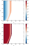Fig. 1 Top panel: growth rates $\mathfrak{I}(\omega )/\mathrm{\Omega }$ for monodisperse streaming instability with St = 0.1 and μ = 0.01. Bottom panel: $\mathrm{d}\text{log}\mathfrak{I}(\omega )/\mathrm{d}\text{log}\mu$ for St = 0.1 at μ = 0.01.

3.2 Polydisperse streaming instability

We now turn to a simple constant size distribution: $${\sigma }^{(0)}(\mathrm{S}\mathrm{t})=\mu {\rho }_{\mathrm{g}}^{(0)}\left\{\begin{array}{ll}\frac{1}{\mathrm{S}{\mathrm{t}}_{\mathrm{m}\mathrm{a}\mathrm{x}}-\mathrm{S}{\mathrm{t}}_{\mathrm{m}\mathrm{i}\mathrm{n}}}\hfill & \mathrm{S}{\mathrm{t}}_{\mathrm{m}\mathrm{i}\mathrm{n}}<\mathrm{S}\mathrm{t}<\mathrm{S}{\mathrm{t}}_{\mathrm{m}\mathrm{a}\mathrm{x}}\hfill \\ 0\hfill & \mathrm{otherwise}.\hfill \end{array}\right\}$$(56)

As in Paper I, we parametrised the minimum and maximum stopping time as St₀(1 ± Δ), where Δ is a measure of the width of the size distribution.

In Fig. 2, we show the growth rates for St₀ = 0.1 and μ = 0.01 and Δ = 0.3. Note Δ = 0 would correspond to the monodisperse result shown in Fig. 1. We also note that this is a size distribution that is much narrower than expected in protoplanetary discs: if the resonant size is 1 mm, Δ = 0.3 means that the minimum size is 0.7 mm and the maximum size is 1.3 mm. In reality, we would expect a distribution that spans many decades (see e.g. McNally et al. 2021). The top panel of Fig. 2 reveals that growing modes for small K_x have disappeared. This is first of all due to the fact that most of this region is dominated by the secular mode in the monodisperse case, for which no equivalent exists for polydisperse dust (see Paardekooper et al. 2020, as well as Paper I). Careful inspection of the wave numbers that give growth reveals that we have also lost the resonant region compared to the monodisperse case. While the bottom panel of Fig. 2 shows that growth is now ∝ μ everywhere, this is not due to the fact that integrating over the resonance yields a regular perturbation: integrating over the resonance actually stabilises the resonant region, which we discuss below. What is left is the non-resonant region to the right of the resonance in Fig. 1, with growth rates that are comparable to the corresponding monodisperse case.

The contribution of the resonance to the growth rate is given by Eq. (55), which reads for z₀ = 0: $$\frac{{\omega }_{1,\mathrm{r}\mathrm{e}\mathrm{s}}}{\mathrm{\Omega }}=-\mathrm{i}\frac{\mu \pi }{8\mathrm{S}{\mathrm{t}}_0\mathrm{\Delta }}\frac{{\widehat{k}}_z^2}{K_x},$$(57) where we also selected the inertial wave with ${\omega }_0=-{\widehat{k}}_z\mathrm{\Omega }$; this is the only one capable of forming a resonance for ${\tilde{z}}_0=0$ and is the one that becomes unstable for the SI. In theory, the inertial wave with positive frequency could lead to non-resonant growth, but this is found not to be the case. From Eq. (57), it is clear that the resonance has a stabilising effect on the system for all wave numbers and Stokes numbers, as long as the size distribution is wide enough that the perturbation is regular (we note that Eq. (57) diverges for Δ → 0, which takes us into the domain of the monodisperse SI).

If growth rates are ∝ μ, which means we are either away from resonance, or the size distribution is wide enough that the contribution of the resonance is regularised, we can use regular eigenvalue perturbation theory to obtain perturbed eigenvalues (see Sect. 2.3). Furthermore, we can then separate the various contributions to the growth rate: dust-density perturbation and the contribution from the relative velocity. As it turns out, the relative velocity perturbation always gives a stabilising contribution, which means that in order to see growth, the contribution of the dust-density perturbation needs to be strong enough.

This is illustrated in Fig. 3, which considers the same two cases as in Figs. 1 and 2 for a fixed K_z = 0.8. The solid and dashed curves correspond to the monodisperse and polydisperse cases, respectively. The total growth rates (blue curves) were calculated exactly, while the contributions from the dust density (orange curves) and drift velocity (green curves) were calculated using perturbation theory (see Sect. 2.3). We note that the drift velocity contribution is always negative; that is, it promotes stability rather than growth, which is why we used the absolute value in Fig. 3. The monodisperse growth rate peaks at the resonance, the location of which can also be inferred from the asymptote in the dust-density perturbation (solid orange curve). Just to the left of the resonance, the dust-density contribution is due to the inertial mode with the opposite sign, which does not have a resonance. In fact, if we adhere to the same mode, the dust-density perturbation is an odd function around the resonance, as can be easily seen from the dust continuity equation. It should be noted, however, that close to the resonance, regular perturbation theory becomes invalid. In the full problem, to the left of the resonance (i.e. smaller K_x), the dust advection mode takes over, while for a large enough K_x growth is no longer possible, as the dust-density contribution (solid orange curve) crosses the stabilising contribution of the drift velocity (solid green curve). It is worth noting that this stabilising effect is not present in the terminal-velocity approximation, where the drift velocity is determined by the pressure gradient only, and as a result the terminal-velocity approximation shows growth up to much larger wave numbers (Lin & Youdin 2017; Paardekooper et al. 2020).

The polydisperse case with Δ = 0.3 follows the monodisperse results closely for the drift perturbation (solid and dashed green curves in Fig. 3). The only significant difference between polydisperse and monodisperse cases occurs around the resonance in the dust density perturbation. Only when the resonance is completely out of the integration domain is growth possible again. This is because of the stabilising effect of the contribution of the resonance (see Eq. (57)). In other words, growing modes exist when $${\omega }_0-k_x{u}_x^{(0)}({\tau }_{\mathrm{s}})=-{\widehat{k}}_z\kappa -k_x\mathrm{\Delta }{u}_x^{(0)}({\tau }_{\mathrm{s}})<0$$(58) for all τ_s in the size distribution. Since $\mathrm{\Delta }{u}_x^{(0)}\approx -2\eta \tau$ for small St and μ, this translates to $k_x<{\widehat{k}}_z\kappa /(2\eta \tau )$. For the parameters of Fig. 3 (St₀ = 0.1, Δ = 0.3 and K_z = 0.8), we find that for K_x > 2.32 the resonance is completely out of the integration domain, which agrees with the point where the dashed blue curve cuts off on the left.

The monodisperse SI disappears for large K_x because the stabilising contribution of the perturbation in drift velocity overtakes the destabilising contribution of the dust density perturbation. This is where the green and orange curves cross in Fig. 3. The limiting K_x can be quantified by first focusing on the monodisperse case. The full expression for ω₁ from eigenvalue pertubation theory is not very enlightening, but we can gain some insight into the limit of small τ_s, where we ignore terms that are quadratic in τ_s: $$\begin{array}{l}\frac{{\omega }_1}{\mu }=\frac{k_x(2\mathrm{\Omega }\mathrm{i}\mathrm{\Delta }{u}_y^{(0)}\pm {\widehat{k}}_z\kappa \mathrm{\Delta }{u}_x^{(0)})}{2{\omega }_{\mathrm{\Delta }}}\left[1+3\mathrm{i}{\tau }_{\mathrm{s}}{\omega }_{\mathrm{\Delta }}\right]\\ -{\omega }_{\mathrm{\Delta }}-\mathrm{i}{\tau }_{\mathrm{s}}{\omega }_{\mathrm{\Delta }}^2-\frac{\mathrm{i}{\kappa }^2}{2}(1+{\widehat{k}}_z^2){\tau }_{\mathrm{s}}\pm {\widehat{k}}_z\kappa (1+2\mathrm{i}{\tau }_{\mathrm{s}}{\omega }_{\mathrm{\Delta }});\end{array}$$(59) here, ${\omega }_{\mathrm{\Delta }}=\pm {\widehat{k}}_z\kappa -k_x\mathrm{\Delta }{u}_x^{(0)}$. The first term on the right is due to the dust-density perturbation, while the rest of the terms are due to the perturbation in relative velocity.

If we focus on the imaginary part of ω₁, plugging in the expression for ω_Δ, we have: $$\begin{array}{l}\frac{\mathrm{\Im }({\omega }_1)}{\mu }=\frac{k_x\mathrm{\Omega }\mathrm{\Delta }{u}_y^{(0)}}{\pm {\widehat{k}}_z\kappa -k_x\mathrm{\Delta }{u}_x^{(0)}}\pm \frac{3{\tau }_{\mathrm{s}}{k}_x{\widehat{k}}_z\kappa \mathrm{\Delta }{u}_x^{(0)}}{2}\\ -{\tau }_{\mathrm{s}}{k}_x^2\mathrm{\Delta }{u}_x^{(0)}{}^2-\frac{(1-{\widehat{k}}_z^2){\kappa }^2{\tau }_{\mathrm{s}}}{2}.\end{array}$$(60)

For small St, $\mathrm{\Delta }{u}_y^{(0)}=\kappa \tau \left|\mathrm{\Delta }{u}_x^{(0)}\right|/2,$,we have the following: $$\begin{array}{l}\frac{2\mathrm{\Im }({\omega }_1)}{{\kappa }^2{\tau }_{\mathrm{s}}\mu }=\frac{\mathrm{\Omega }}{\kappa }\frac{k_x|\mathrm{\Delta }{u}_x^{(0)}|/\kappa }{k_x|\mathrm{\Delta }{u}_x^{(0)}|/\kappa \pm {\widehat{k}}_z}\mp 3{\widehat{k}}_z{k}_x|\mathrm{\Delta }{u}_x^{(0)}|/\kappa \\ -2k_x^2|\mathrm{\Delta }{u}_x^{(0)}{|}^2/{\kappa }^2-(1-{\widehat{k}}_z^2).\end{array}$$(61)

We have zero growth (i.e. $\mathfrak{I}({\omega }_1)=0$) when $$\pm \frac{\mathrm{\Omega }}{{\widehat{k}}_z^2\kappa }+2q^3\pm 5q^2+2q\mp 1=0,$$(62) with $q=\frac{k_x\left|\mathrm{\Delta }{u}_x^{(0)}\right|}{\kappa {\widehat{k}}_z}$. If we take the Keplerian case κ = Ω, we find that in the limit ${\widehat{k}}_z\to 1$ the relevant solution has q = 2, which makes the limiting horizontal wavenumber K_x = 10, which agrees with the location of the right edge of the region of growth towards large K_z in Fig. 1. While this edge roughly follows the constant q curve, which has the same shape as the resonance condition, deviations start to occur at smaller K_z. At K_z = 0.8, the case studied in Fig. 3, q = 2 corresponds to K_x = 2.8, while the edge of the region of positive growth rates is located at K_x = 3.5, as correctly predicted by the solution of the cubic Eq. (62). This means that we are far enough away from the resonance to use regular perturbation theory to predict the edge of growth.

In the polydisperse case, we have an integration over stopping time: $$\mathrm{\Im }({\omega }_1)=\frac{1}{{\rho }_{\mathrm{g}}^{(0)}}\frac{{\kappa }^4{\widehat{k}}_z^2}{2k_x^2}\int {\sigma }^{(0)}q\left[\frac{q}{q\pm 1}\mp 3{\widehat{k}}_z^{2}q-2{\widehat{k}}_z^2{q}^2-1+{\widehat{k}}_z^2\right]\mathrm{d}q,$$(63) where we again took κ = Ω and used $\mathrm{\Delta }{u}_x^{(0)}=-2\eta \tau$ to make the integration over q rather than τ_s. The condition that growth vanishes is now given by an average over the size distribution for all terms. For the particular size distribution Eq. (56), the limiting wave number is very close to the monodisperse case (see Fig. 3). For size distributions that are dominated by larger (smaller) stopping times, the limiting wave number will move to the left (right). Hence, including larger stopping times in the size distribution makes it more difficult for the SI to survive in the polydisperse case.

A reasonable approximation to the maximum growth rate in the polydisperse case with size distribution Eq. (56) can be obtained by taking the growth rate of the corresponding monodisperse case, but at the wave number where the resonance is just outside the integration domain. In Fig. 3, this corresponds to K_x = 2.4. We find that $$\frac{\mathrm{\Im }({\omega }_1)}{\mathrm{\Omega }}=\frac{\mu \mathrm{S}{\mathrm{t}}_0}{2}\left[\frac{1-\mathrm{\Delta }}{\mathrm{\Delta }}+\frac{{\widehat{k}}_z^2}{1-\mathrm{\Delta }}\left(4-\mathrm{\Delta }-\frac{2}{1-\mathrm{\Delta }}\right)\right].$$(64)

For Δ → 0, the first term in square brackets blows up because we are approaching the resonance, rendering the analysis invalid. For Δ → 1, the last term dominates, stabilising the flow. For intermediate values of Δ, the term in square brackets is O(1), and we find a growth rate of $\mathfrak{I}({\omega }_1)/\mathrm{\Omega }\sim \mu$, which is a factor of $\sqrt{\mu }$ lower than in the monodisperse case (Squire & Hopkins 2018b). Growth is no longer due to the resonance, but due to a regular perturbation of an inertial wave. From the approximate relation Eq. (64), we find that this intermediate regime is bounded by Δ < 0.5.

As with the acoustic drag instability (see Paper I), for size distributions that are narrow enough the quasi-monodisperse regime exists, whereby the system acts as if the dust is monodisperse. How narrow the size distribution needs to be for this to happen is illustrated in Fig. 4. The wave numbers are chosen such that we are at the resonance in the monodisperse case, and towards smaller values of Δ it is clear that growth rates are $\propto \sqrt{\mu }$. For wider size distributions growth vanishes at the location of the resonance up to Δ = 0.4, at which point we do not see any growth even for μ = 0.1. Since the real part of the monodisperse frequency perturbation is given by ${\widehat{k}}_z\sqrt{\mu /2}\mathrm{\Omega }$ (Squire & Hopkins 2018b), we find that the quasi-monodisperse regime exists for $$\mathrm{\Delta }<\frac{{\widehat{k}}_z\sqrt{\mu }}{2\sqrt{2}{K}_x\mathrm{S}{\mathrm{t}}_0}.$$(65)

If we restrict ourselves to the resonance corresponding to St₀, this becomes $$\mathrm{\Delta }<\sqrt{\frac{\mu }{2}}.$$(66)

In Fig. 4, this corresponds to where the curves are horizontal. So while the quasi-monodisperse regime is more accessible for smaller stopping times and smaller horizontal wave numbers, the condition for resonant growth only depends on the dust-to-gas ratio (see Eq. (66)). This agrees with the work of Paardekooper et al. (2020), whose case with μ = 0.5 and a wide size distribution showed no growth at resonant wave numbers (their Fig. 5).

Fig. 2 Top panel: growth rates for polydisperse streaming instability for μ = 0.01, St0 = 0.1, and Δ = 0.3. Bottom panel: $\mathrm{d}\text{log}\mathfrak{I}(\omega )/\mathrm{d}\text{log}\mu$ for St0 = 0.1, Δ = 0.3 at μ = 0.01.

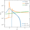Fig. 3 Growth rate, in units of Ω−1, at Kz = 0.8, for the monodisperse case of Fig. 1 (solid curves) and the polydisperse case of Fig. 2 (dashed curves). Yellow curves: contribution of dust-density perturbation to the growth rate. Green curves: contribution of relative velocity perturbation to the growth rate (absolute contribution, since it is a stabilising effect). Blue curves: total growth rate.

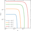Fig. 4 Growth rates of SI with St0 = 0.1 and varying width of the size distribution at Kx = 2 and Kz = 0.85, which in the monodisperse case is the location of the resonance.

3.3 Summary

The resonance that gives rise to the SI in the monodisperse regime is an enemy of polydisperse growth. Only for very narrow size distributions do we recover the monodisperse regime (see Eq. (66)). For slightly wider size distributions, integrating over the resonance regularises the perturbation, making the SI no longer an RDI. Despite the stabilising effect of the resonance, a band of unstable wave numbers can persist for size distributions of moderate width, with growth rates of ~μSt₀ that are non-resonant. From Eq. (64), for this band to persist for all ${\widehat{k}}_z$ requires Δ < 0.5. For wide size distributions including particles of very small Stokes numbers the SI switches off completely for μ ≪ 1, an effect that is captured in Eq. (64). Therefore, the polydisperse, low-μ SI is unlikely to play a role in realistic settings of planet formation. The non-resonant, high-μ variant of the SI, which we do not study here, is more promising in the polydisperse regime, if the size distribution is favourable (McNally et al. 2021).

4 Settling instability

We now let z₀ ≠ 0 and study the settling instability. While the streaming instability has received more attention in the context of planet formation, the settling instability is interesting for several reasons: it generally grows faster than the SI and can grow fast in the RDI regime of μ ≪ 1, and growth rates can be independent of stopping time (Squire & Hopkins 2018b). Moreover, it does not seem to be affected by the existence of a distribution of dust sizes, and convergence with the number of dust species is much more easily achieved than for the SI (Krapp et al. 2020).

We start off by setting z₀ = H = c/Ω, where H is a measure of the vertical thickness of the gas disc. This is also the value considered in Krapp et al. (2020). We note that this implies a settling velocity that is larger than the radial drift velocity by more than an order of magnitude: $$\frac{\mathrm{\Delta }{u}_z}{\mathrm{\Delta }{u}_x}\approx \frac{z_0{\mathrm{\Omega }}^2{\tau }_{\mathrm{s}}}{2\eta {\tau }_{\mathrm{s}}}=\frac{z_0}{H}\frac{c\mathrm{\Omega }}{2\eta }\approx 16\frac{z_0}{H},$$(67) where in the last step we used our choice of η/(cΩ) = 10^−3/2. We also work with a lower than usual dust-to-gas ratio, μ = 10⁻⁴. This is because the higher growth rates of the settling instability lead to higher values of μ yielding perturbations in the eigenvalues that are no longer small (basically because ${\tilde{z}}_0\gg 1$). Choosing such a small value of μ ensures that we remain safely in the regime where resonant drag theory is fully valid.

In Fig. 5, we show growth rates for the monodisperse DSI with St = 0.1. The resonance clearly stands out as the red curve with the highest growth rates (a similar pattern was shown in Krapp et al. (2020) for St = 0.01), which even for μ = 10⁻⁴ easily reach $\mathfrak{I}(\omega )/\mathrm{\Omega }=0.01$. In the bottom panel of Fig. 5, the resonance stands out as the white curve, showing slower growth with μ compared to the red regions of regular (non-resonant) perturbations.

Towards the bottom of Fig. 5, the white curve splits into two branches. This becomes more obvious in this wave-number range if we consider smaller values of z₀. In Fig. 6, we show growth rates for St₀ = 0.1 and μ = 10⁻⁴, which are similar to those of Fig. 5 but at z₀/H = 0.001. The top panel shows results for the monodisperse case, and the resonant branches show up as white regions of high growth. The bottom branch, which is barely visible in Fig. 5 and not shown in Fig. 1 of Krapp et al. (2020), is the branch that in the limit of z₀ → 0 gives rise to the streaming instability. Towards small K_z, it already maps onto the SI resonant location seen in Fig. 1, but we note that the growth rates are lower due to the smaller μ value considered in Fig. 6.

In the bottom panel of Fig. 6, the polydisperse case with a constant size distribution and St/St₀ ∈ [0.5, 1.5] is considered. Here, we see that the SI branch suffers its usual fate of quenching under a size distribution. As in the pure SI case, integrating over the resonance destroys growth. On the other hand, the resonance due to settling survives a size distribution. In this case, since it is the other inertial wave that creates the resonance, the resonance has a positive contribution to growth in the polydisperse case. This can be seen from Eq. (55), as the vertical settling is in resonance with the inertial wave that has the opposite frequency to the radial drift. As a result, this branch survives relatively unscathed, even for rather wide size distributions.

This is further illustrated in Fig. 7, where we return to z₀/H = 1 and fix K_z = 0.2. From Fig. 5, we see that for this value of K_z we cross two resonances at K_x ≈ 0.3 and K_x ≈ 3. In the latter case, the two branches of resonance come together into what was called the double resonant angle in Squire & Hopkins (2018b), which is the subject of the next subsection. The resonance at K_x ≈ 0.3 is only active for z₀ ≠ 0, and in Fig. 7 the blue curves, indicating the monodisperse case, clearly show the growth-rate peak at the resonance. Moreover, when changing the dust-to-gas ratio by a factor of ten (solid vs. dotted curves), growth at the resonance only changes by a factor of $\sqrt{10}$, which is the hallmark of a resonant drag instability.

The polydisperse cases shown in Fig. 7 have a constant size distribution with St/St₀ ∈ [1 Δ, 1 + Δ], as usual. For Δ = 0.1, the resonance can still be identified, but for Δ = 0.5 it is smeared out considerably. Importantly, growth rates are now everywhere ∝ μ even for a relatively narrow size distribution with δ = 0.1, there is a difference in growth rate of a factor of ten between the solid and dotted orange curves. This shows that the perturbation is now regular, that is, no longer resonant. Furthermore, from Eq. (55) we expect the following contribution of the resonance: ∝ 1/Δ; this agrees with the differences between Δ = 0.1 and Δ = 0.5 around K_x = 0.3.

The difference in maximum growth rate around the resonance between the monodisperse case and the polydisperse case will therefore strongly depend on μ, since the former scales as $\sqrt{\mu }$ and the latter as μ. In Fig. 7, for μ = 10⁻⁴ the maximum monodisperse growth rate is a factor of 20 higher than the polydisperse case with Δ = 0.5, but for μ = 10⁻³ it is only a factor of 5.5 higher.

Further experiments with narrower size distributions showed that for δ < 0.01 we enter the quasi-monodisperse regime for μ = 10⁻⁴. This is consistent with the requirement $\mathrm{\Delta }\lesssim \sqrt{\mu }$, which is similar to the SI (see Eq. (66)).

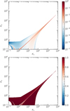Fig. 5 Top panel: growth rates for monodisperse settling instability with St = 0.1, μ = 0.0001 and z0/H = 1. Bottom panel: $\mathrm{d}\text{log}\mathfrak{I}(\omega )/\mathrm{d}\text{log}\mu$ at μ = 0.0001.

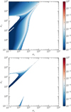Fig. 6 Growth rates for settling instability for μ = 10−4 and z0/H = 0.001. Top panel: monodisperse with St = 0.1. Bottom panel: polydisperse with St0 = 0.1 and size distribution width Δ = 0.5.

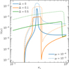Fig. 7 Growth rates for the DSI with z0/H = 1 and St0 = 0.1, at fixed vertical wavenumber Kz = 0.2. Solid curves: μ = 10−4, dashed curves: μ = 10−3. Different colors indicate different widths of the size distribution.

4.1 Double resonance

One of the interesting features of the DSI is that growth rates approach infinity at the double resonant angle where k · Δu = 0. This is where the two resonant branches merge, as seen in the top panel of Fig. 6.

If we want the resonance to behave in a quasi-monodisperse fashion, we again need the spread in k · Δu due to the size distribution to be much smaller than the perturbed gas-wave velocity, which for the double resonance is ω_mono/Ω = −(2StμK_x)^1/3/2 (Squire & Hopkins 2018b). In the limit of μ → 0, the relative velocities are $$\mathrm{\Delta }{u}_x=-\frac{2\eta }{\mathrm{\Omega }}\frac{\mathrm{S}\mathrm{t}}{1+\mathrm{S}{\mathrm{t}}^2},$$(68) $$\mathrm{\Delta }{u}_z=\mathrm{\Omega }{z}_0\mathrm{S}\mathrm{t}.$$(69)

If we take a narrow size distribution with St/St₀ ∈ [1 - δ/2, 1 + δ/2], we find that to the first order in δ, we obtain a spread of $$\frac{\mathrm{\Delta }(\mathbf{k}\cdot \mathrm{\Delta }\mathbf{u})}{\mathrm{\Omega }}=\left[K_z{\tilde{z}}_0\mathrm{S}{\mathrm{t}}_0-2K_x\frac{\mathrm{S}{\mathrm{t}}_0}{1+\mathrm{S}{\mathrm{t}}_0^2}\right]\delta +\frac{4K_x\mathrm{S}{\mathrm{t}}_0^3\delta }{{(1+\mathrm{S}{\mathrm{t}}_0^2)}^2}.$$(70)

The term in square brackets is zero at the resonant Stokes number St₀. For a narrow size distribution, δ ≪ 1, one can develop a series in δ, with the monodisperse result given by ω_mono. In order to stay close to the monodisperse regime, that is, quasi-monodisperse, we require integrals of $$\int \frac{{\sigma }^{(0)}f(\mathrm{S}\mathrm{t})}{{\omega }_{\mathrm{m}\mathrm{o}\mathrm{n}\mathrm{o}}-\mathbf{k}\cdot \mathrm{\Delta }{\mathbf{u}}^{(0)}}\mathrm{d}\mathrm{S}\mathrm{t},$$(71) to form a converging series in δ. With the help of Eq. (70) and the expression for ω_mono evaluated close to St₀, we easily find that we need $$\delta \ll {\left(\frac{1}{3}+\frac{8K_x\mathrm{S}{\mathrm{t}}_0^3}{(1+\mathrm{S}{\mathrm{t}}_0^2){(2\mathrm{S}{\mathrm{t}}_0\mu K_x)}^{1/3}}\right)}^{-1}.$$(72)

The quasi-monodisperse case is most easily reached for small K_x, a low Stokes number, and a high dust-to-gas ratio. Some examples are shown in Fig. 8. When δ_lim ~ 1, growth rates at the double resonance will be unaffected, even by a wide size distribution. As discussed in Squire & Hopkins (2018b), the double resonance only plays a role for $$K<\frac{{\left(\frac{\pi }{2}-|{\theta }_{\mathrm{r}\mathrm{e}\mathrm{s}}|\right)}^3}{\mu \mathrm{S}\mathrm{t}},$$(73) where θ_res = arctan(Δu_z/Δu_x) is the double resonant angle. This is the wave number where the curves in Fig. 8 are cut off on the left. From the figure, we see that the smaller Stokes number setup never leaves the quasi-monodisperse regime: we expect to see similar growth rates for polydisperse dust to the monodisperse case, even for relatively wide size distributions. Due to the strong Stokes number dependence of Eq. (72), the situation is very different for St₀ = 0.1. For μ = 10⁻⁴, the quasi-monodisperse regime is out of reach for wide size distributions for all wave numbers, while for μ = 10⁻² it is attainable only for small K_x. Importantly, the DSI shows highest growth rates for large K_x (Squire & Hopkins 2018b).

We show numerically calculated growth rates around the double resonance in Fig. 9. The blue curves, indicating monodisperse results (which are a factor of ten apart in μ) show a difference of a factor of ten in the growth rate at the left end of the plot, indicating non-resonant growth. At the growth peaks, they only differ by a factor 2.17 ≈ 10^1/3, clearly indicating growth ∝ μ^1/3 at the double resonant angle.

If we take a size distribution with Stokes numbers between St₀(1 - Δ) and St₀(1 + Δ) and Δ < 1 (but not necessarily small), from Fig. 8 we expect the quasi-monodisperse regime to be confined to Δ ⪅ 0.1 at K_x ≈ 1500. Indeed, the narrow size distribution with Δ = 0.01 (orange curve in Fig. 9) closely follows the monodisperse case around the resonance (but not towards the non-resonant regime at the left end of the figure). A wider size distribution with Δ = 0.7 (green curves in Fig. 9) still shows the highest growth rates close to the resonant location, but growth is reduced compared to the monodisperse case, and it is no longer ∝ μ^1/3. In fact, it appears that the maximum growth rate is ∝ μ^1/2, but further work is necessary to establish the exact dependence on μ.

It should be noted that the high wave numbers that are the domain of the double resonance can be problematic for the fluid approximation for the dust. Moreover, they are particularly susceptible to viscous damping, which we explore below.

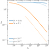Fig. 8 Limiting width of a constant size distribution with St/St0 ∈ [1 - δ, 1 + δ] (see Eq. (72)) for different central Stokes numbers and dust-to-gas ratios.

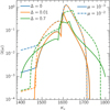Fig. 9 Growth rates for DSI at z0 = H, St0 = 0.1 and Kz = 100. Different colours indicate different widths of the size distribution, and we consider μ = 10−3 (solid curves) and μ = 10−2 (dashed curves). The location of the double resonance in the monodisperse regime, in the limit μ = 0 and St → 0, is at Kx ≈ 1580.

4.2 Gas viscosity and dust diffusion

We finally add gas viscosity and dust diffusion to the problem, in the same way as in McNally et al. (2021), following the formulation of Chen & Lin (2020). As mentioned in McNally et al. (2021), this model does not capture turbulent clumping, or the effect of dust on gas turbulence, but only represents average effects of the turbulence. With this in mind, we show growth rates for the DSI for z₀ = H and μ = 10⁻⁴ for varying levels of viscosity in Fig. 10.

From the inviscid case (leftmost panels in Fig. 10), we see the disappearance of the SI branch of the resonance and the smearing out of the DSI-related resonance. Towards larger K_x, we see that the double resonance is far less affected, indicating that the maximum growth rate in the polydisperse regime will be comparable to the monodisperse case.

If we start to increase gas viscosity and associated dust diffusion, we see that the double resonance disappears first (middle panels of Fig. 10); this is due to the fact that it is confined to high wave numbers and therefore more susceptible to diffusion. This is also where the maximum growth rate starts to differ between the monodisperse and polydisperse case. For α = 10⁻⁵, the difference is almost an order of magnitude.

4.3 Numerical convergence in the DSI

A different approach than that presented in Paardekooper et al. (2021) to solving roots of the dispersion relation Eq. (B.13), which involves integrals over stopping time, is to first discretize the back-reaction on the gas: $$\begin{array}{l}\frac{\mathrm{i}}{{\rho }_{\mathrm{g}}^{(0)}}\int \frac{{\sigma }^{(0)}}{{\tau }_{\mathrm{s}}}\left[\mathrm{\Delta }{\mathbf{u}}^{(0)}\frac{\widehat{\sigma }}{{\sigma }^{(0)}}+\widehat{\mathbf{u}}-\widehat{\mathbf{v}}\right]\mathrm{d}{\tau }_{\mathrm{s}}\equiv \int f({\tau }_{\mathrm{s}})\mathrm{d}{\tau }_{\mathrm{s}}\\ \approx \sum _{n}f({\tau }_{\mathrm{s},n})w_n,\end{array}$$(74) with nodes τ_s,n and weights w_n. For wide size distributions, it is convenient to perform the integral in log space. There is further freedom in choosing equidistant nodes (Krapp et al. 2019, 2020), or Gauss-Legendre nodes. For N integration nodes, we end up with a straightforward eigenvalue problem with matrix size (4 + 4N) × (4 + 4N), which can be solved using standard methods. This was termed the ‘direct solver’ in McNally et al. (2021).

Krapp et al. (2019) and Paardekooper et al. (2021) showed that for the streaming instability, in large regions of parameter space this method fails to converge, or converges very slowly with N. For N ≳ 4000, the problem quickly becomes computationally intractable. The problem can be traced to the nastiness of the integrand (Paardekooper et al. 2021) that is close to singular. Not only does that mean that linear growth rates are more difficult to obtain, there is a danger that numerical simulations (that cannot afford to have 10 000s of dust species) will pick up spurious growing modes that come to dominate the simulation.

In Krapp et al. (2020), it was shown that the situation looks better for the settling instability: the maximum growth rate over a range of wave numbers (k_x, k_z) ∈ 2π[1, 1000]/H converges for N ≳ 32 with μ = 0.01 and z₀/H = 1. Here, we present some additional numerical experiments and some more details on where and when we can expect fast convergence.

In the left panel of Fig. 11 we show growth rates calculated using the direct solver with N = 100. This panel can be compared to the bottom left panel of Fig. 10. It is obvious that there is a lot of numerical noise, in particular towards the lower left part of the figure. The dotted structure around K_x = K_z = 0.5 are artefacts resulting from integrating over the DSI-related resonance. We also note that the streaming instability branch is present, even though it should not be (see Fig. 10). This is again due to integration errors over the resonance (Krapp et al. 2019; Paardekooper et al. 2021).

In the right panel of Fig. 11, we show a convergence study at fixed wave numbers around the double resonant angle. For a relatively narrow size distribution, convergence is obtained even for N = 10, while for the wider size distribution, numerical errors prevent convergence. It seems as though the amplitude of the noise goes down with N, so perhaps convergence can be reached at much larger N than that considered here.

The situation improves if we increase the dust-to-gas ratio to μ = 0.01. In particular, this takes the double resonant angle into the quasi-monodisperse regime, which is easier for standard integration methods to deal with. A case similar to that of Fig. 12 was studied in Krapp et al. (2020) (their Fig. 2), which showed that the maximum growth rate converges for N Ω 32. They used a different size distribution, but we also find that the maximum growth rate, which occurs towards the double resonant angle at the highest K_x, does not change significantly upon increasing N. However, the top panel of Fig. 12 shows numerical artefacts for smaller K_x, similar to those seen in Fig. 11. Again, these are caused by integrating over the resonance using a method that is not suited to dealing with near-singularities. This is something to be aware of in numerical simulations of the DSI; as is the case for the SI, spurious modes may grow, albeit more slowly than the double resonant modes if these are present.

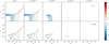Fig. 10 Growth rates for μ = 10−4 and z0 = H for different levels of viscosity. The top row shows monodisperse results; the bottom row polydisperse ones with a wide size distribution (Δ = 0.99).

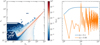Fig. 11 Left: growth rates for μ = 10−4 and z0 = H, calculated with N = 100 discrete dust sizes sampling a size distribution with Δ = 0.99. Right: convergence with N close to double-resonant angle with Kx = 16 007 and Kz = 1000 for Δ = 0.1 and Δ = 0.99.

4.4 Summary

The polydisperse settling instability differs from the polydisperse streaming instability in two important ways. First of all, the resonant branch associated with the settling velocity gives a positive contribution when integrated over. This means that, unlike the SI, the polydisperse DSI survives in the limit of μ ≪ 1. Integrating over the resonance regularises the perturbation such that the growth rate becomes ∝ μ, rather than $\propto \sqrt{\mu }$ as in the monodisperse case.

Second, at the double resonant angle, growth can be less sensitive to having a size distribution, at least for maximum Stokes numbers that are much smaller than unity (see Fig. 8). In those cases, the perturbation to the gas wave is strong enough that the instability remains in the quasi-monodisperse regime. Unfortunately, as the double resonance is confined to relatively large wave numbers, it is more susceptible to diffusion.

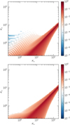Fig. 12 Growth rates for DSI with μ = 0.01, St0 = 0.1, and a constant size distribution with Δ = 0.99. Top panel: calculation using direct method and 32 dust species equidistant in log space. Bottom panel: calculation using method of Paardekooper et al. (2021).

5 Discussion and conclusion

We present linear calculations of two resonant drag instabilities in the polydisperse regime that are thought to be important in protoplanetary discs: the streaming instability and the settling instability. The results can provide a starting point for non-linear simulations, which will in the end determine if these instabilities lead to clumping and planetesimal formation, for example (e.g. Krapp et al. 2020). We will consider this in a forthcoming paper.

Several important simplifications were made to make the problem tractable. First of all, we have only considered the limit μ ≪ 1. It is important to note that this is not the regime usually studied for the SI, where it is usually assumed that dust settling has led to a dust-to-gas ratio of the order of unity, for example. This regime was studied in the polydisperse case in Krapp et al. (2019), Zhu & Yang (2021), and McNally et al. (2021), among others. For μ ≪ 1, the SI is a resonant drag instability, while it changes character for μ > 1 (Squire & Hopkins 2018b). By keeping μ ≪ 1, we can make firm contact with RDI theory, leading to a deeper understanding of the polydisperse SI.

We have only considered very simple (i.e. constant) size distributions. The dependence of the form of the size distribution on the growth rates is different for each instability. Since the contribution of the resonance to the SI is negative, and the dust density contribution to the growth rate is dominated by the resonance, it is virtually impossible to pick a size distribution that leads to growth. Basically, one would have to exclude the ‘resonant size’ completely from the size distribution. For larger values of μ, the resonance is less dominant, and there the form of the size distribution can have an impact (McNally et al. 2021). A similar story holds for the DSI, but in a positive way: since the contribution of the resonance is positive, it will be hard to find a size distribution that reduces the growth rates significantly compared to the constant size distribution considered here. For reference, for the acoustic drag instability, the contribution of the resonance can be positive or negative, depending on the asymmetry of the size distribution with respect to the resonant size (see Paper I).

It may seem paradoxical that to see growth for the PSI, the corresponding resonant size needs to be excluded from the size distribution, even though the resonance is responsible for growth in the SI. The following thought experiment might help clarify why this is the case. Let us consider the monodisperse streaming instability at wave number k_mono, Stokes number St_mono, and eigenvalue ${\omega }_{\text{mono}}\approx {\omega }_{\text{inertial}}=k_{x,\text{mono}}{v}_{\text{g}x}^{(0)}-{\widehat{k}}_{z,\text{mono}}\kappa$. Take the wave number to meet the resonant condition so that ω_inertial = k_mono · u(0), and the dust-to-gas ratio to be μ_mono ≪ 1. Now add a polydisperse component with μ_poly ≪ μ_mono. Because μ_poly ≪ μ_mono, the polydisperse component is not able to appreciably change the eigenvalue from ω_mono. Now consider the size density perturbation in the polydisperse component: $$\frac{\widehat{\sigma }}{{\sigma }^{(0)}}=\frac{{\mathbf{k}}_{\mathrm{m}\mathrm{o}\mathrm{n}\mathrm{o}}\cdot \widehat{\mathbf{u}}}{{\omega }_{\mathrm{m}\mathrm{o}\mathrm{n}\mathrm{o}}-{\mathbf{k}}_{\mathrm{m}\mathrm{o}\mathrm{n}\mathrm{o}}\cdot {\mathbf{u}}^{(0)}}.$$(75)

This term, multiplied by Δu(0), enters the back-reaction $\widehat{b}$ under the integral sign, and is the main driver of instability. Assume for the sake of argument that $k_{\text{mono}}\cdot \widehat{u}<0$ for all St. The denominator is $${\omega }_{\mathrm{m}\mathrm{o}\mathrm{n}\mathrm{o}}-k_{x,\mathrm{m}\mathrm{o}\mathrm{n}\mathrm{o}}{u}_x^{(0)}\approx -{\widehat{k}}_{z,\mathrm{m}\mathrm{o}\mathrm{n}\mathrm{o}}\kappa +2\eta {\tau }_{\mathrm{s}}{k}_{x,\mathrm{m}\mathrm{o}\mathrm{n}\mathrm{o}},$$(76) which is an odd function of τ_s around the resonant stopping time. This means that Stokes numbers smaller than St_mono will provide a positive contribution to the back-reaction (we note that the multiplication with Δu(0) changes the sign), while Stokes numbers greater than St_mono will give a negative contribution to the back-reaction. The closer to the resonance, the stronger these contributions are. This means that, on one side of the resonance, Stokes numbers arbitrarily close to the resonance have a strongly negative effect on the growth rate of the instability, even though growth is caused by the monodisperse component at the resonance.

The reason for this apparent paradox is that the polydisperse component is forced at the wrong frequency everywhere except exactly at the resonance. The total effect of the polydisperse component can be found by integration over the size distribution. Whether the resonance has a positive or negative contribution now crucially depends on the numerator in the size-density perturbation Eq. (75) and its dependance on the Stokes number. This causes the difference between the SI resonance and the DSI resonance, where in the case of the SI the resonance damps growth, and in the case of the DSI it promotes growth. In reality, we do not have dust made up of a dominant monodisperse component and a polydisperse component of negligible mass, but the issue remains that most of the polydisperse dust will be forced at the wrong frequency.

A very important simplification is that we have considered only unstratified shearing boxes. For the SI, this restricts the analysis to close to the mid plane, while for the DSI it means that we can only consider timescales that are short compared to the settling time. The fully stratified case is more complex to deal with, because setting up an equilibrium requires including a turbulence model to keep the dust from settling (Lin 2021). An unstratified model can be used to delineate effects of diffusion – but it is clear that future models should include stratification – to bring linear results in closer contact with numerous non-linear simulations (see e.g. Li & Youdin 2021; Klahr & Schreiber 2021; Lim et al. 2024, for recent results).

We only considered a very simple drag law with constant stopping time. A more general form of Epstein drag was given in Hopkins & Squire (2018), where the stopping time depends both on gas density and relative velocity between gas and dust. For the two instabilities discussed in this paper, the streaming instability and the settling instability, gas-density perturbations are almost absent: a common approximation is that the gas is in fact incompressible (e.g. Youdin & Goodman 2005; Squire & Hopkins 2018b). Furthermore, for drift velocities that are highly subsonic, corrections to the stopping time due to the relative velocity are very small. For the streaming instability, it is definitely safe to take the stopping time to be constant. The same is true for the settling instability as long as the Stokes numbers remain much smaller than unity.

The thermodynamics of the disc was modelled in a simple way, assuming the gas is isothermal. More realistic models were considered in Lehmann & Lin (2023), which showed that in many cases, the DSI can be stabilised by vertical buoyancy, while new instabilities can arise as well. How these effects interact with dust-size distribution remains to be explored.

Given that the contribution of the resonance to the back-reaction integral is different for the three instabilities considered so far, it would be interesting to explore different resonant instabilities (Squire & Hopkins 2018b) with a size distribution. The three instabilities studied here lead to three different categorisations:

• The resonance gives a negative contribution to the growth rate (SI).

• The resonance gives a positive contribution to the growth rate (DSI). A wide size distribution makes the perturbation regular rather than singular.

• The contribution of the resonance can be positive or negative depending on the size distribution (ARDI, see Paper I). The resulting perturbation is regular for wide size distributions.

Apart from the double resonant angle for the DSI, even very narrow size distributions around the resonance lead to non-resonant behaviour; typically only for $\mathrm{\Delta }/S_0\lesssim \sqrt{\mu }$ can we expect to achieve something close to the monodisperse result.

In conclusion, for realistically wide size distributions, dust-gas instabilities will mostly show non-resonant growth in the limit μ ≪ 1. The classical streaming instability does not survive at all in this limit, as the resonance has a stabilising effect. The settling instability does survive, with growth rates that are very similar to the monodisperse case, but with a stronger dependence on μ compared to monodisperse results.

Data availability

All data used to create figures in this work are available at https://doi.org/10.4121/810f163a-b786-4366-ad9b-5794d71c4ede

Acknowledgements

We want to thank the anonymous referee for an insightful report. This project has received funding from the European Research Council (ERC) under the European Union’s Horizon Europe research and innovation programme (Grant Agreement No. 101054502). This work made use of several open-source software packages. We acknowledge numpy (Harris et al. 2020), matplotlib (Hunter 2007), scipy (Virtanen et al. 2020), and PSITOOLS (McNally et al. 2021). We acknowledge 4TU.ResearchData for supporting open access to research data.

Appendix A Governing equations for the inertial wave RDI

We start from a standard stratified shearing box; Eqs. (1)-(5) with the appropriate shearing box accelerations $${\mathbf{\alpha }}_{\mathrm{g}}=2\eta \widehat{\mathbf{x}}-2\mathbf{\Omega }\times {\mathbf{v}}_{\mathrm{g}}-\nabla {\mathrm{\Phi }}_{\mathrm{t}\mathrm{o}\mathrm{t}},$$(A.1) $${\mathbf{\alpha }}_{\mathrm{d}}=-2\mathbf{\Omega }\times {\mathbf{v}}_{\mathrm{g}}-\nabla {\mathrm{\Phi }}_{\mathrm{t}\mathrm{o}\mathrm{t}},$$(A.2) where the potential Φ_tot = −SΩx² + Ω²z²/2 (S is the shear rate of the disc), and the term involving η is representing a global radial pressure gradient in the disc: $${\partial }_t{\rho }_{\mathrm{g}}+\nabla \cdot ({\rho }_{\mathrm{g}}{\mathbf{v}}_{\mathrm{g}})=0,$$(A.3) $$\begin{array}{l}{\partial }_t{\mathbf{v}}_{\mathrm{g}}+({\mathbf{v}}_{\mathrm{g}}\cdot \nabla ){\mathbf{v}}_{\mathrm{g}}=2\eta \widehat{\mathbf{x}}-\frac{\nabla p}{{\rho }_{\mathrm{g}}}+\frac{1}{{\rho }_{\mathrm{g}}}\int \sigma \frac{\mathbf{u}-{\mathbf{v}}_{\mathrm{g}}}{{\tau }_{\mathrm{s}}}\mathrm{d}{\tau }_{\mathrm{s}}\\ -2\mathbf{\Omega }\times {\mathbf{v}}_{\mathrm{g}}-\nabla {\mathrm{\Phi }}_{\mathrm{t}\mathrm{o}\mathrm{t}},\end{array}$$(A.4) $${\partial }_t\sigma +\nabla \cdot (\sigma \mathbf{u})=0,$$(A.5) $${\partial }_t\mathbf{u}+(\mathbf{u}\cdot \nabla )\mathbf{u}=-\nabla {\mathrm{\Phi }}_{\mathrm{t}\mathrm{o}\mathrm{t}}-2\mathbf{\Omega }\times \mathbf{u}-\frac{\mathbf{u}-{\mathbf{v}}_{\mathrm{g}}}{{\tau }_{\mathrm{s}}}.$$(A.6)

The equation of state for the gas is taken to be isothermal as usual: $p=c_{\text{g}}^2{\rho }_{\text{g}}$.

Consider a domain centered on z = -z₀ < 0³, with vertical extent L_z ≪ z₀, so that we can take the vertical gravitational acceleration to be constant: $${\mathrm{\Phi }}_{\mathrm{t}\mathrm{o}\mathrm{t}}=-S\mathrm{\Omega }{x}^2-{\mathrm{\Omega }}^2{z}_{0}z=\mathrm{\Phi }-{\mathrm{\Omega }}^2{z}_{0}z.$$(A.7)

References

- Binney, J., & Tremaine, S. 2008, Galactic Dynamics, 2nd edn. (Princeton: Princeton University Press) [Google Scholar]
- Chen, K., & Lin, M.-K. 2020, ApJ, 891, 132 [Google Scholar]
- Draine, B. T., Dale, D. A., Bendo, G., et al. 2007, ApJ, 663, 866 [NASA ADS] [CrossRef] [Google Scholar]
- Goldreich, P., & Lynden-Bell, D. 1965, MNRAS, 130, 125 [Google Scholar]
- Harris, C. R., Millman, K. J., van der Walt, S. J., et al. 2020, Nature, 585, 357 [NASA ADS] [CrossRef] [Google Scholar]
- Hawley, J. F., Gammie, C. F., & Balbus, S. A. 1995, ApJ, 440, 742 [Google Scholar]
- Hopkins, P. F., & Squire, J. 2018, MNRAS, 480, 2813 [Google Scholar]
- Hopkins, P. F., Squire, J., & Seligman, D. 2020, MNRAS, 496, 2123 [NASA ADS] [CrossRef] [Google Scholar]
- Hunter, J. D. 2007, Comput. Sci. Eng., 9, 90 [NASA ADS] [CrossRef] [Google Scholar]
- Johansen, A., Oishi, J. S., Mac Low, M.-M., et al. 2007, Nature, 448, 1022 [Google Scholar]
- Klahr, H., & Schreiber, A. 2021, ApJ, 911, 9 [NASA ADS] [CrossRef] [Google Scholar]
- Krapp, L., Benítez-Llambay, P., Gressel, O., & Pessah, M. E. 2019, ApJ, 878, L30 [Google Scholar]
- Krapp, L., Youdin, A. N., Kratter, K. M., & Benítez-Llambay, P. 2020, MNRAS, 497, 2715 [NASA ADS] [CrossRef] [Google Scholar]
- Landau, L. D. 1946, J. Phys. (USSR), 10, 25 [Google Scholar]
- Latter, H. N., & Papaloizou, J. 2017, MNRAS, 472, 1432 [CrossRef] [Google Scholar]
- Lehmann, M., & Lin, M.-K. 2023, MNRAS, 522, 5892 [CrossRef] [Google Scholar]
- Lesur, G., Flock, M., Ercolano, B., et al. 2023, in ASP Conf. Ser., 534, 465 [NASA ADS] [Google Scholar]
- Li, R., & Youdin, A. N. 2021, ApJ, 919, 107 [NASA ADS] [CrossRef] [Google Scholar]
- Lim, J., Simon, J. B., Li, R., et al. 2024, ApJ, 969, 130 [NASA ADS] [CrossRef] [Google Scholar]
- Lin, M.-K. 2021, ApJ, 907, 64 [Google Scholar]
- Lin, M.-K., & Youdin, A. N. 2017, ApJ, 849, 129 [NASA ADS] [CrossRef] [Google Scholar]
- Magnan, N., Heinemann, T., & Latter, H. N. 2024a, MNRAS, 529, 688 [NASA ADS] [CrossRef] [Google Scholar]
- Magnan, N., Heinemann, T., & Latter, H. N. 2024b, MNRAS, 534, 3944 [NASA ADS] [CrossRef] [Google Scholar]
- McNally, C. P., Lovascio, F., & Paardekooper, S.-J. 2021, MNRAS, 502, 1469 [NASA ADS] [CrossRef] [Google Scholar]
- Paardekooper, S.-J., & Aly, H. 2025, A&A, 696, A53 [NASA ADS] [CrossRef] [EDP Sciences] [Google Scholar]
- Paardekooper, S. J., & Papaloizou, J. C. B. 2008, A&A, 485, 877 [NASA ADS] [CrossRef] [EDP Sciences] [Google Scholar]
- Paardekooper, S.-J., McNally, C. P., & Lovascio, F. 2020, MNRAS, 499, 4223 [CrossRef] [Google Scholar]
- Paardekooper, S.-J., McNally, C. P., & Lovascio, F. 2021, MNRAS, 502, 1579 [NASA ADS] [CrossRef] [Google Scholar]
- Rucska, J. J., & Wadsley, J. W. 2023, MNRAS, 526, 1757 [NASA ADS] [CrossRef] [Google Scholar]
- Schaffer, N., Johansen, A., & Lambrechts, M. 2021, A&A, 653, A14 [NASA ADS] [CrossRef] [EDP Sciences] [Google Scholar]
- Squire, J., & Hopkins, P. F. 2018a, ApJ, 856, L15 [NASA ADS] [CrossRef] [Google Scholar]
- Squire, J., & Hopkins, P. F. 2018b, MNRAS, 477, 5011 [Google Scholar]
- Virtanen, P., Gommers, R., Oliphant, T. E., et al. 2020, Nat. Methods, 17, 261 [Google Scholar]
- Weidenschilling, S. J. 1977, MNRAS, 180, 57 [Google Scholar]
- Yang, C.-C., & Zhu, Z. 2021, MNRAS, 508, 5538 [NASA ADS] [CrossRef] [Google Scholar]
- Youdin, A. N., & Goodman, J. 2005, ApJ, 620, 459 [Google Scholar]
- Zhu, Z., & Yang, C.-C. 2021, MNRAS, 501, 467 [Google Scholar]
- Zhuravlev, V. V. 2019, MNRAS, 489, 3850 [NASA ADS] [Google Scholar]
Strictly speaking, the corresponding height would be -z0; this is to ensure the acceleration is in the direction of the mid plane. This particular choice is consistent with Krapp et al. (2020).
Since our parameter η is dimensional by choice, with dimensions of acceleration, η/(cΩ) is equivalent to Π in Krapp et al. (2020).
This choice makes the final result consistent with Krapp et al. (2020)