| Issue |
A&A
Volume 696, April 2025
|
|
|---|---|---|
| Article Number | A224 | |
| Number of page(s) | 9 | |
| Section | Stellar structure and evolution | |
| DOI | https://doi.org/10.1051/0004-6361/202553867 | |
| Published online | 23 April 2025 | |
Revealing two orthogonally polarized spectral components in Vela X-1 with IXPE
1
Department of Physics and Astronomy, FI-20014 University of Turku, Finland
2
Space Research Institute, Russian Academy of Sciences, Profsoyuznaya 84/32, Moscow, 117997
Russia
3
Institut für Astronomie und Astrophysik, Universität Tübingen, Sand 1, D-72076 Tübingen, Germany
4
Astrophysics, Department of Physics, University of Oxford, Denys Wilkinson Building, Keble Road, Oxford, OX1 3RH
UK
⋆ Corresponding author: This email address is being protected from spambots. You need JavaScript enabled to view it.
Received:
23
January
2025
Accepted:
19
March
2025
Abstract
Polarimetric observations of X-ray pulsars (XRPs) have provided us with the key to unlocking their geometrical properties. Thanks to the Imaging X-ray Polarimetry Explorer (IXPE), the geometries of several XRPs have been determined, providing new insights into their emission mechanisms and magnetic field structures. The polarimetric properties of Vela X-1 have a clear dependence on energy, showing a 90° swing in the polarization angle (PA) between low and high energies. Due to the complex energy-dependent nature of the polarization properties, until now it was not possible to determine the pulsar geometry. In this work we present the results of a detailed analysis of the pulse-phase-resolved polarization properties of Vela X-1 at different energies. By separating the polarimetric analysis into low and high energy ranges, we are able to disentangle the contributions of the soft and hard spectral components to the polarization, revealing the pulse phase dependence of the polarization degree and PA in each energy band. The PA pulse-phase dependence at high energies (5−8 keV) allows us, for the first time, to determine the pulsar geometry in Vela X-1. Based on the fit with the rotating vector model, we estimate the pulsar spin position angle to be around 127° and the magnetic obliquity to be 13°. We discuss two possible scenarios that could explain the 90° swing in the PA between high and low energies: a two-component spectral model and vacuum resonance.
Key words: accretion / accretion disks / magnetic fields / polarization / stars: neutron / pulsars: individual: Vela X-1 / X-rays: binaries
© The Authors 2025
 Open Access article, published by EDP Sciences, under the terms of the Creative Commons Attribution License (https://creativecommons.org/licenses/by/4.0), which permits unrestricted use, distribution, and reproduction in any medium, provided the original work is properly cited.
This article is published in open access under the Subscribe to Open model. This email address is being protected from spambots. You need JavaScript enabled to view it. to support open access publication.
1. Introduction
Accreting X-ray pulsars (XRPs) are highly magnetized neutron stars (NSs) that accrete matter from massive stellar companions (see Mushtukov & Tsygankov 2024 for a recent review). They provide us with indispensable laboratories for studying the processes related to the complex interplay between accreting matter, radiation, and the strong magnetic field of the NS itself. As a consequence of the strong magnetic field, the accreting matter is confined to small regions around the magnetic poles of the NS, which leads to the appearance of pulsed X-ray emission as the NS rotates. The strong magnetic field is also the main cause of the highly polarized X-ray emission expected from these sources. Due to the birefringence of highly magnetized plasma, the emission can be treated in terms of two normal polarization modes: the ordinary mode (O-mode) and the extraordinary mode (X-mode). The significant difference in the opacity of these two modes (below the cyclotron energy) means that, in theory, a large degree of polarization is expected to be observed from these sources (Meszaros et al. 1988; Caiazzo & Heyl 2021). The launch of the Imaging X-ray Polarimetry Explorer (IXPE) in December 2021 has provided a new tool for examining the X-ray polarimetric properties of XRPs. Importantly for XRPs, their geometrical properties can be determined from the additional information encrypted in the behavior of the polarization properties as a function of the pulsar phase.
Several XRPs have been observed by IXPE (see the recent review by Poutanen et al. 2024a): Her X-1 (Doroshenko et al. 2022; Heyl et al. 2024; Zhao et al. 2024), Cen X-3 (Tsygankov et al. 2022), X Persei (Mushtukov et al. 2023), 4U 1626−67 (Marshall et al. 2022), Vela X-1 (Forsblom et al. 2023, hereafter Paper I), GRO J1008−57 (Tsygankov et al. 2023), EXO 2030+375 (Malacaria et al. 2023), LS V +44 17 (Doroshenko et al. 2023), GX 301−2 (Suleimanov et al. 2023), Swift J0243.6+6124 (Poutanen et al. 2024b), and SMC X-1 (Forsblom et al. 2024). Their polarization properties show a pattern of a rather low (∼10%) linear polarization degree (PD), even in the pulse-phase-resolved polarimetric data, calling earlier theoretical predictions into question. Additionally, the geometrical properties of the majority of XRPs observed by IXPE have been determined by modeling the pulse-phase dependence of the polarization angle (PA) with the rotating vector model (RVM; Radhakrishnan & Cooke 1969; Meszaros et al. 1988; Poutanen 2020).
IXPE observations of the wind-accreting high-mass X-ray binary (HMXB) Vela X-1 (also known as 4U 0900−40) did reveal a relatively low phase-averaged PD of 2.3 ± 0.4% with a PA of  in the 2−8 keV energy band (Paper I). The phase-averaged energy-resolved polarimetric analysis provided the most interesting results, revealing a clear energy dependence of the polarization properties in the IXPE 2−8 keV energy band, with a 90° PA swing at around 3.4 keV, a unique behavior among the XRPs observed by IXPE. The PD shows a decrease from around 4% at 2−3 keV down to zero at 3.4 keV, and then increases to about 10% at 7−8 keV with a PA rotated by ∼90° relative to that at low energies. A phase-resolved polarimetric analysis also found a PD in the range 0−9% with the PA varying between −80° and 40°. However, the complicated nature of the PA pulse-phase dependence cannot be explained using the RVM, and, therefore, the pulsar geometry could not be determined for Vela X-1.
It is important to note that additional polarized contributions may arise in the system, for example from reflection off the NS surface, the accretion disk, the disk wind, or the stellar wind of the companion star (see Tsygankov et al. 2022, for discussion). This could lead to these polarized components being entangled with the polarized emission produced at the NS magnetic poles, resulting in complications when interpreting the behavior of the pulse-phase dependence of the polarization properties. Particularly, the bright transient XRPs LS V +44 17 and Swift J0243.6+6124 both require the addition of a second, constant (un-pulsed) polarized component to explain their PA pulse-phase dependence within the framework of the RVM, which thereby allowed the determination of their geometrical properties (Doroshenko et al. 2023; Poutanen et al. 2024b).
Vela X-1, a bright and persistent XRP, is often considered the archetypal wind accretor and remains one of the most studied HMXBs (Chodil et al. 1967). It is a binary system consisting of a NS and the stellar companion GP Vel, a B0.5Ib supergiant (Quaintrell et al. 2003). Vela X-1 has a spin period of 283 s (McClintock et al. 1976) and an orbital period of 8.964 d (Ulmer et al. 1972; van Kerkwijk et al. 1995), showing eclipses that last for about 2 d, with a lower limit on the orbital inclination of i = 73° (van Kerkwijk et al. 1995). Vela X-1 is deeply embedded in the stellar wind of its companion star, and the X-ray luminosity is known to be variable on all timescales, with an average value of around LX ∼ 4 × 1036 erg s−1 (Staubert et al. 2004; Kreykenbohm et al. 2008). Vela X-1 is known to display so-called soft excess, which has been attributed to the contribution of an additional low-energy component to the overall spectral continuum. The source of this low-energy component has not been confirmed but has been hypothesized to originate from the dense stellar wind surrounding the NS, or from thermal emission at the NS surface (see, e.g., Hickox et al. 2004).
Considering the results of the energy-resolved polarimetric analysis of Vela X-1 in Paper I and the well-established presence of a soft excess in the source spectrum, the energy-dependent nature of the polarization may be due to two separate polarized components of different origins. This results in the complex behavior displayed by the PA pulse-phase dependence. Consequently, the pulse-phase dependence of the PA at low and high energies should exhibit different behaviors. The RVM can then be applied to the PA pulse-phase dependence of the component associated with the emission from the accretion region at the NS magnetic poles (i.e., the high-energy component). Here, we attempt to disentangle the contribution of the two components to the energy dependence of Vela X-1’s polarization properties via a detailed spectro-polarimetric analysis using observations made by IXPE.
2. Data
IXPE is an observatory launched in December 2021 as a NASA/Italian Space Agency (ASI) mission, providing imaging polarimetry over the 2−8 keV energy range (Weisskopf et al. 2022). IXPE consists of three grazing incidence telescopes, each consisting of a mirror module assembly, which focuses X-rays onto a focal-plane polarization-sensitive gas pixel detector unit (DU). In addition to measuring the sky coordinates, time of arrival, and energy of each detected photon, it also measures the direction of the photo-electron, which enables polarimetric analyses.
The results of the analysis of the IXPE data are published in Paper I, based on two observations of Vela X-1 conducted by IXPE (01002501, 02005801) on 2022 April 15–21 and November 30–December 6 with total effective exposures of 280 and 270 ks, respectively. The following analysis is based on the same (level-2) dataset, which has been downloaded from the HEASARC archive1, and processed with the IXPEOBSSIM package version 30.2.1 using the CalDB version 20211209:v13 for observation 1, and for observation 2, using the CalDB version 20220702:v13.
The source photons were extracted from a region of radius Rsrc = 70″. We used the barycorr tool from the FTOOLS package to correct event arrival times to the barycenter of the Solar System. To correct for orbital motion in a binary system, we used the orbital parameters for Vela X-1 provided by the Fermi Gamma-ray Burst Monitor2. Because of the high count rate from the source, we did not subtract the background (Di Marco et al. 2023). Considering the similarities between the two IXPE observations, we combined the data into one single set, excluding the eclipse data from observation 1. We used the information provided in Paper I to phase-tag the events, with the phase difference between the pulse profiles from the first and second observations determined by cross-correlating the profiles (using the implementation provided by the Python library NUMPY).
For the spectro-polarimetric analysis, source I, Q, and U Stokes spectra were extracted using the xpbin tool’s PHA1, PHA1Q, and PHA1U algorithms, producing a dataset of nine spectra per observation, three for each DU. The I, Q, and U spectra from observations 1 and 2 were subsequently combined using the mathpha tool. Corresponding response files for the observations were combined using the addrmf and addarf tools. Finally, the subsequent spectro-polarimetric analysis is performed using XSPEC package (Arnaud 1996), version 12.14.0. Stokes I spectra have been binned to have a minimum of 30 counts per energy channel. The same energy binning was subsequently applied to the Stokes Q and U spectra. The total set of nine spectra was fitted with XSPEC using χ2 statistics, and model parameter uncertainties are presented at the 68.3% confidence level (1σ) unless stated otherwise.
3. Results
3.1. Spectral model with two polarized components
Some XRPs display a soft component in their spectra, in addition to the power-law component, which is frequently modeled as a blackbody or thermal bremsstrahlung (Hickox et al. 2004). These spectral components (i.e., hard and soft components) may have entirely separate origins. The hard (power-law) component is associated with the accretion region at the NS surface, while the soft component may have a different origin (see Sect. 4.1), which may or may not display pulse-phase dependence. A spectro-polarimetric analysis extracting the individually polarized properties of the soft and hard components can be utilized to disentangle the properties of the spectral continuum.
Several phenomenological models have been utilized to describe Vela X-1 spectral continuum (see Kretschmar et al. 2021, and references therein). The X-ray emission below 10 keV can be well described by a simple absorbed power law with an iron line at 6.4 keV. In addition to this, Vela X-1 is known to display a soft excess below 3 keV (Haberl 1994). Due to the restricted energy range covered by IXPE and the energy resolution of the instrument (Weisskopf et al. 2022), we used a simplified model and did not include an iron line. Including an iron line at 6.4 keV results in a normalization of the line component that is consistent with zero (the other parameters are consistent whether the iron line is included or not). Hence, we did not include this component in the final model (neither in the phase-averaged nor the phase-resolved analysis).
The high-energy component was fitted with a simple power-law model powerlaw. In order to account for the soft excess below 3 keV, we fit this low-energy component with the bremss model in XSPEC (kT ∼ 0.5 keV; Haberl 1994). The interstellar absorption affecting the continuum was introduced using the model tbabs with the abundances from Wilms et al. (2000). This was combined with the polconst polarization model, which assumes energy-independent PD and PA, applied to the individual components (bremss and powerlaw components). In order to achieve an acceptable fit, a partial covering absorption model tbpcf was introduced as well, which applies an added column density to a fraction of the continuum model (Kretschmar et al. 2021). The re-normalization constant, const, was used to account for the possibility of discrepancies between the different DUs, and for DU1 it was fixed to unity. The final spectral model
 (1)
(1)
was used as the model for the initial phase-averaged spectro-polarimetric fitting.
The results of the phase-averaged spectro-polarimetric analysis using two separately polarized emission components are given in Table 1 and the I (flux) spectra are shown in Fig. 1. The steppar command in XSPEC was used to produce confidence contours and the contour plots for the PD and PA are shown in Fig. 2. The results demonstrate that the two-component spectral model effectively explains the findings of the phase-averaged energy-resolved analysis. Namely, the difference in PA between the components is close to 90°. Figure 1 shows that the contribution of these components at ∼3.5 keV is equal. Around this energy, the PD is zero, as the contribution from the two components with nearly equal PD cancels out. This is also in line with what was observed in the phase-averaged energy-resolved analysis (see Paper I).
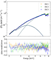 |
Fig. 1. Unfolded energy spectra (Stokes I parameter) of Vela X-1 in EFE representation, using a two-component model fit to the IXPE dataset. The solid, dashed, and dotted lines show the total model spectrum, the thermal bremsstrahlung component, and the power-law component, respectively. The bottom panel shows the fit residuals. |
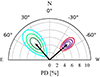 |
Fig. 2. Polarization vector of Vela X-1 from the results of the phase-averaged spectro-polarimetric analysis of the IXPE dataset. Contours at 68.3%, 95.45%, and 99.73% confidence are shown for the bremss and powerlaw components in greenish and reddish colors, respectively. |
Ideally, we would like to examine the phase-resolved energy dependence of the polarization properties. However, we do not have enough statistics to perform a detailed phase-resolved spectro-polarimetric analysis using a model with two separately polarized components. Therefore, we adopted a simplified approach by dividing the total energy range into low- and high-energy parts and used simple models for the spectral fitting.
3.2. Analysis of low- and high-energy emission
Utilizing the results from the phase-averaged analysis with two polarized components, we confined the fit to low and high energies separately. From the point where the contributions from the two components to the total polarized flux are equal (i.e., where the PD is equal to zero), we determined the break-off point between the energy ranges. To minimize the contribution of different spectral components to the nearby band, the 3−5 keV range was completely excluded from the analysis. The final energy ranges used for the phase-resolved spectro-polarimetric fitting (with minimal contribution from the other component) are 2−3 and 5−8 keV. The values of the tbabs and tbpcf parameters were fixed to that of the phase-averaged results.
For the spectro-polarimetric analysis at low energies, we used a simplified model:
 (2)
(2)
which was applied to each phase bin. The results are given in Table 2 and shown in the left panels of Fig. 3. Normalized Stokes q and u parameters are extracted using the xpbin tool’s pcube algorithm included in the IXPEOBSSIM package, which has been implemented according to the formalism by Kislat et al. (2015). However, low counting statistics make it impossible to constrain the behavior of the PD and PA. For the polconst model, the PD is consistent with zero for most of the phase bins, and the PA is unconstrained. However, for the few phase bins where we can significantly detect the PD, we can compare the results with the ones from the high-energy analysis (see below).
Spectro-polarimetric parameters in different pulse-phase bins for the low- (LE) and high-energy (HE) bands.
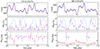 |
Fig. 3. Results of the phase-resolved spectro-polarimetric analysis of Vela X-1 based on the IXPE data at low energies (LE; 2−3 keV; left) and high energies (HE; 5−8 keV; right). Top panels: Pulse profiles (in counts) corresponding to the low- and high-energy ranges. Middle and bottom panels: Pulse-phase dependence of the PD and PA, respectively. The NuSTAR pulse profile in the 15−45 keV energy band is displayed in the PD panels (light blue). The orange curve in the PA panel shows the best-fit RVM to the data in the high-energy range. |
The phase-resolved spectro-polarimetric analysis at high energies (5−8 keV) was performed using the model:
 (3)
(3)
The results are given in Table 2 and shown in the right panels of Fig. 3. As can be seen from the figure, this results in a nicely structured behavior of both the PD and PA, where the pulse-phase dependence of the PA displays a single sine wave over the pulse phase (compared to the complicated behavior of the PA in Paper I). Therefore, we can use these results to model the PA phase dependence with the RVM model and determine the pulsar geometry for Vela X-1 for the first time. It is worth noting that different energy ranges (3.5−8, 4−8, and 4.5−8 keV) all give us consistent results for the phase-dependence of the PA.
Due to the fact that we observe a 90° difference in the PA between the two components in the phase-averaged analysis, we would like to examine if the same behavior is observable in the phase-resolved analysis. This can be achieved by comparing the polarization properties of the two components in each phase bin. We observe significant polarization in both energy ranges only in the 0.600−0.650 phase bin. Comparing the PA of the components in this phase bin, we see a difference being close to 90° (see Fig. 4). For the remaining phase bins, the difference between the PAs is consistent with 90°, with the PA unconstrained for a large number of phase intervals at low energies.
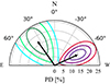 |
Fig. 4. Polarization vectors of Vela X-1 from the results of the phase-resolved spectro-polarimetric analysis for the phase interval 0.600−0.650. Contours at 68.3, 95.45, and 99.73% confidence are shown for the bremss and powerlaw components in greenish and reddish colors, respectively. |
The pulse profile of Vela X-1 is known to show both a unique and complex five-peaked structure at lower energies. However, the pulse profile evolves to a simpler two-peak structure at higher energies. Using NuSTAR data in the 15−45 keV energy range, we compared the high-energy pulse profile to the results of the phase-resolved spectro-polarimetric analysis, for both the low- and high-energy polarization results (see Fig. 3). The pulse-phase dependence of the PD shows a noticeable correlation (albeit with some shift in the phase) with the high-energy pulse profile, with the flux minima roughly corresponding to the minima in the PD.
4. Discussion
The observations of XRPs made by IXPE have revealed a more complicated picture of these sources in terms of their polarization properties than what has been predicted by theory. Significantly lower PDs than expected provide an incentive to revisit theoretical models and consider different mechanisms that may contribute. Several possible processes that may be involved in producing the polarization observed in XRPs were discussed in Tsygankov et al. (2022). Consequently, the observed polarization properties may in fact be affected by a multitude of different processes in the immediate environment of the NS, as well as processes related to the interaction of photons under the extreme conditions of a highly magnetized plasma. These processes may in turn lead to a more complex spectrum, where contributions from different components arise and require their own interpretation.
Considering the complex nature of the pulse-phase-dependent polarization properties of Vela X-1, it is likely that an interplay of several factors is responsible. Below, we discuss possible explanations for Vela X-1’s unique energy-dependent polarimetric behavior in terms of two separate mechanisms. First, we consider the possibility that the polarization may be attributed to two independently polarized spectral components, with a 90° difference in PA between them. For the second mechanism, the 90° difference in the PA is considered to be introduced by vacuum resonance, where a conversion from one polarization mode to the other occurs. Finally, the disentanglement of the pulse-phase-dependent polarization properties of the high-energy component from that of the low-energy component offers us the opportunity to determine the geometrical parameters of the pulsar.
4.1. Two spectral components
The existence of soft excess in Vela X-1 is well established and, as mentioned in the introduction, different origins to it have been proposed but have yet to be confirmed. The soft excess appears as an additional contribution at low energies to the hard spectral continuum. The general spectral continuum of Vela X-1 can be described using two components: a power law and a thermal bremsstrahlung, which accounts for the additional low-energy flux from the source. The hard (power-law) spectral component of emission from Vela X-1 is believed to originate from the accretion region (i.e., the accretion mound at the NS magnetic poles); while the origin of the soft component is unknown, several possibilities have been hypothesized. Hickox et al. (2004) provided an extensive review of the possible origin of soft excesses in XRPs in general and in Vela X-1 in particular. For Vela X-1, the soft excess is believed to originate from either the stellar wind surrounding the NS or the thermal emission from the NS surface.
It is difficult to draw any conclusions about the origin of the soft component based on its polarization properties. Because of the fact that we observe a similar level of pulsed fraction in the low-energy as in the high-energy bands, we can conclude that the low-energy component is pulsed and should originate from a sufficiently compact region. Therefore, it is possible that the low-energy component is produced by thermal emission from compact regions at the NS surface, in the immediate vicinity of the base of the accretion mound and illuminated by it, resulting in a 90° difference in PA compared to that of the high-energy component.
4.2. Vacuum polarization
Vela X-1 is a relatively low-luminosity XRP operating in the subcritical accretion regime (see, e.g., Basko & Sunyaev 1976; Mushtukov et al. 2015). The polarization of its radiation can thus be considered within the framework of a toy model for an accretion-heated NS atmosphere, initially proposed for Her X-1 (Doroshenko et al. 2022). In this model, the upper atmospheric layers are overheated by plasma deceleration via Coulomb collisions (e.g., Zel’dovich & Shakura 1969; Zane et al. 2000; Suleimanov et al. 2018; González-Caniulef et al. 2019).
We considered a toy model describing the upper layers of the NS atmosphere heated by the accreting particles. We assumed that the base atmosphere is isothermal and the upper layers are overheated. We took a predefined temperature dependence on the column density, m, in the atmosphere:
 (4)
(4)
where Tup is the temperature of the upper overheated layer, Tlow is the temperature of the underlying atmosphere, and mup is the transition column density between these two layers. We considered a fully ionized pure hydrogen atmosphere with the gas pressure P = mg determined from the integral of the hydrostatic equilibrium equation, where g is the surface gravity. For simplicity, we ignored the external ram pressure of the accretion flow as well as the radiation pressure. Next, we solved the radiation transfer equation in the two polarization modes with the standard boundary conditions. The corresponding opacities, including vacuum polarization and mode conversion at the vacuum resonance, are incorporated following van Adelsberg & Lai (2006). The code is described in detail in Suleimanov et al. (2009).
For the model calculations, we assumed a NS mass of 1.4 M⊙ and a radius of R = 12 km, with a surface magnetic field strength of B = 3 × 10¹² G, which corresponds to the energy of the observed cyclotron feature in Vela X-1. We find that the polarization of the emergent radiation in the energy range 2−8 keV can be sufficiently low at certain model parameters, as was previously observed for Her X-1 (Doroshenko et al. 2022). Here, we considered a single model with the following parameters: Tup = 6 × 10⁸ K, Tlow = 107 K, and mup = 0.75 g cm−2.
The results of the radiation transfer computations in two normal modes for this model are presented in Figs. 5, 6, and 7. The emergent spectrum of the model is compared with the model spectrum of the isothermal atmosphere (upper panel of Fig. 5). It is clear that the upper overheated layer adds the optically thin emission to the thermal blackbody-like radiation of the isothermal atmosphere. This optically thin radiation is mainly emitted in the O-mode because the absorption (free-free) opacity is larger in this mode (see the middle panels in Figs. 5 and 6). It is interesting that the vacuum polarization is insignificant at the photon energies above 8 keV, and converts X- and O-modes to each other at low energies below 2 keV. And there is a relatively broad energy region 2−8 keV where vacuum polarization makes the intensities in X- and O-modes close to each other resulting in a close to zero PD (Fig. 5, bottom panel). These results are connected to the vacuum polarization properties, which we discuss below.
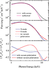 |
Fig. 5. Energy dependences of the fluxes and polarization. Upper panel: Emergent spectra from the isothermal atmosphere (red curve) and from the atmosphere with the hot upper layer (black curve). Middle panel: Emergent spectra in the normal modes for the model with the hot upper layer with (solid curves) and without (dashed curves) vacuum polarization taken into account. Bottom panel: Energy dependence of the PD for the hot layer model with (blue curve) and without (red curve) vacuum polarization taken into account. |
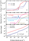 |
Fig. 6. Dependences of the mean intensities (upper panel), scattering and free-free opacities (middle panel), and the optical thickness (bottom panel) of the normal modes on the column density, m, with (solid curves) and without (dashed curves) vacuum polarization taken into account. |
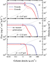 |
Fig. 7. Dependences of the fluxes in the normal modes at different photon energies on column density m with (solid curves) and without (dashed curves) vacuum polarization taken into account. The mass density is also shown with the solid light gray curves (right axes). |
The importance of vacuum polarization for radiation transfer in highly magnetized model atmospheres of NSs wasinvestigated in detail by Lai & Ho (2002, 2003a,b). The main conclusions are the following. Virtual electron-positron pairs in a strong magnetic field change the dielectric tensor of the plasma and, as a result, the plasma opacity, especially in the X-mode (see Fig. 6, middle panel). The opacity increases significantly at the so-called vacuum resonance depth and in the deeper layers, whereas in the more upper layers, it decreases. As a result, the optical thickness over the whole atmosphere changes (Fig. 6, bottom panel), which leads to different distributions of mean intensities over depth (Fig. 6, top panel). The intensities in the two modes are partially converted to each other at the vacuum resonance depth. We show in Fig. 6 the results obtained for the photon energy at which the vacuum resonance produces an equality of intensities of the two modes.
The vacuum resonance occurs at the depth where the contributions of the vacuum polarization and the plasma to the dielectric tensor become equal. The plasma density at this depth must satisfy the following condition
 (5)
(5)
where E is the photon energy in keV and B14 = B/1014 G. It means that for the given magnetic field strength the depth of the vacuum resonance depends strongly on the photon energy.
The modes are almost completely converted to each other after passing the vacuum resonance. At low photon energies, the vacuum resonance takes place in the upper layers, which are optically thin in both modes. In this case the emergent fluxes in the modes just also converted to each other (see Fig. 7, bottom panel). If the vacuum resonance occurs in the deep layers where both modes are thermalized with equal intensities, its presence does not affect the spectrum of the emergent radiation in any way.
The most interesting case is when the vacuum resonance takes place at the depth where the X-mode has already formed and is in an optically thin state, whereas the radiation in O-mode is still in the process of formation. Then the intensity in the X-mode drops to the O-mode level and stays constant. Whereas the intensity in O-mode increases to the level of X-mode intensity, but then continues to decrease with depth (see Fig. 6, top panel). Therefore, at some photon energy, these intensities and the emergent fluxes can become equal to each other (see Fig. 7, middle panel). In a standard atmosphere, the density decreases smoothly toward the surface, and the described situation occurs in a narrow range of photon energies. But in the transition layer between the normal atmosphere and the overheated layer, the density gradient is significant and the emergent fluxes in both modes could be close to each other in the relatively broad photon energies (see the top panels of Figs. 6 and 7).
We do not pretend to explain the whole X-ray energy spectrum of Vela X-1 using this toy model. The cyclotron emission together with the Compton scattering have to be included for that. We just demonstrate that the overheated upper layers of the atmosphere and the transition layer can create conditions under which the polarization of the emergent radiation will be close to zero in a relatively wide range of energies below 10 keV. We also note that the suggested toy model is a variation of the two-component model discussed in the previous subsection. The change of the polarization at the energies below 2.5 keV occurs due to the contribution of the optically thin emission of the overheated layer.
4.3. Determination of the pulsar geometry
Vacuum birefringence (Gnedin et al. 1978; Pavlov & Shibanov 1979) causes the polarized radiation in the NS magnetosphere to propagate in the O- and X-modes, representing oscillations of the electric field parallel and perpendicular to the plane made up by the local magnetic field and photon momentum, respectively. The polarization plane rotates as the radiation travels through the NS magnetosphere, up to the adiabatic radius (Heyl et al. 2003; Taverna et al. 2015), which is located at ∼20 NS radii for the magnetic field strength typical for XRPs (Heyl & Caiazzo 2018; Taverna & Turolla 2024). At such a distance, the dipole magnetic field component will dominate. Under these conditions, the RVM is applicable and can be used to constrain the pulsar geometry (Meszaros et al. 1988). For a slowly rotating NS, the PA does not depend on the PD of the radiation escaping from the surface of the NS, or any other details.
The geometrical properties of several XRPs observed by IXPE have already been obtained (Doroshenko et al. 2022, 2023; Tsygankov et al. 2022, 2023; Mushtukov et al. 2023; Malacaria et al. 2023; Suleimanov et al. 2023; Heyl et al. 2024; Zhao et al. 2024; Poutanen et al. 2024b; Forsblom et al. 2024). If the radiation is assumed to be dominated by O-mode photons, the PA is (see Eq. (30) in Poutanen 2020)
 (6)
(6)
where χp is the position angle (measured from north to east) of the pulsar angular momentum, ip is the inclination of the pulsar spin to the line of sight, θ is the magnetic obliquity (i.e., the angle between the magnetic dipole and the spin axis), and ϕ0 is the phase when the northern magnetic pole passes in front of the observer. If instead, the radiation escapes predominantly in the X-mode, the position angle of the pulsar angular momentum is χp ± 90°.
We can fit the RVM to the pulse-phase-dependent PA obtained from the spectro-polarimetric analysis of the high-energy component using the affine invariant Markov chain Monte Carlo ensemble sampler EMCEE package of PYTHON (Foreman-Mackey et al. 2013). Because the PA is not normally distributed, we used the probability density function of the PA, ψ, from Naghizadeh-Khouei & Clarke (1993):
![Mathematical equation: $$ \begin{aligned} G(\psi ) = \frac{1}{\sqrt{\pi }} \left\{ \frac{1}{\sqrt{\pi }} + \eta \mathrm{e}^{\eta ^2} \left[1 + \mathrm{erf}(\eta )\right]\right\} \mathrm{e}^{-p_0^2/2}. \end{aligned} $$](/articles/aa/full_html/2025/04/aa53867-25/aa53867-25-eq17.gif) (7)
(7)
Here, p0 = p/σp is the measured PD in units of the error, ![Mathematical equation: $ \eta = p_0 \cos[2(\psi-\psi_0)]/\sqrt{2} $](/articles/aa/full_html/2025/04/aa53867-25/aa53867-25-eq18.gif) , ψ0 is the central PA obtained from XSPEC, and erf is the error function. We applied the likelihood function L = ΠiG(ψi) with the product taken over all phase bins. The covariance plot for the parameters is shown in Fig. 8. The RVM provides an overall good fit to the PA of the high-energy component. The magnetic obliquity and the pulsar position angle are accurately determined as θ = 13° ±6° and χp = 127° ±3°, respectively. The inclination is less well constrained; however, the estimate of
, ψ0 is the central PA obtained from XSPEC, and erf is the error function. We applied the likelihood function L = ΠiG(ψi) with the product taken over all phase bins. The covariance plot for the parameters is shown in Fig. 8. The RVM provides an overall good fit to the PA of the high-energy component. The magnetic obliquity and the pulsar position angle are accurately determined as θ = 13° ±6° and χp = 127° ±3°, respectively. The inclination is less well constrained; however, the estimate of  deg is consistent with the lower limit on the orbital inclination of 73° given by van Kerkwijk et al. (1995).
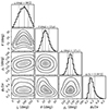 |
Fig. 8. Corner plot of the posterior distribution for the parameters of the RVM model fitted to the PA values obtained from the phase-resolved spectro-polarimetric analysis of the high-energy component. The two-dimensional contours correspond to 68.3, 95.45, and 99.73% confidence levels. The histograms show the normalized one-dimensional distributions for a given parameter derived from the posterior samples. The vertical dashed lines represent the mode of the distribution (central line) and the lower and upper quartiles (68% confidence interval). The mode is calculated using a Gaussian kernel density estimate with a bandwidth of 0.1. |
Bulik et al. (1995) found evidence of non-antipodal polar caps in Vela X-1 using a spectral model of an inhomogeneous magnetized atmosphere fitted to phase-resolved data obtained with Ginga. The rotation axis and the mean magnetic axis were found to be relatively close (i.e., they found small magnetic obliquities for both caps) and are seen at a large inclination with respect to the line of sight. The angle between the center of the polar cap and the rotational axis for caps 1 and 2 were found to be 22° ±12° and 168° ±12°, respectively, for the most significant fits. These results are in line with what is displayed in Fig. 8, where the results of the RVM-fitting similarly give us a small magnetic obliquity, with θ = 13° ±6°.
5. Summary
Vela X-1 represents a unique case among the XRPs observed by IXPE so far. IXPE uncovered a clear energy dependence of its PD and PA, with the PD reaching zero at around 3.4 keV, corresponding to a switch in the PA of 90°. We have proposed an explanation for the curious case of Vela X-1’s energy-dependent polarization properties. The results of our study can be summarized as follows:
-
The energy dependence of the polarimetric properties of Vela X-1 can be explained by a two-component model in which the low- and high-energy components have different polarization properties, with the PA differing by 90°.
-
Our phase-averaged polarimetric analysis based on a spectral model consisting of two perpendicularly polarized components, a power-law component, and a thermal bremsstrahlung component, effectively explains the energy dependence of polarization, including the 90° switch in PA between the components. At around 3.4 keV, the contribution from the two components to the polarized flux is equal, resulting in zero total PD, consistent with what was observed in Paper I.
-
Our phase-resolved polarimetric analysis, in which we separated the low (2−3 keV) and high (5−8 keV) energies, allowed us to examine the phase-resolved polarization properties in these two energy ranges. At low energies, the polarization in the phase-resolved data is predominantly unconstrained. At high energies, the PD and PA both display a nice structure over the pulse phase. The PD shows a correlation with the high-energy pulse profile, and the PA displays a single sine wave over the pulse period.
-
We propose two different scenarios to explain the 90° difference in the PA between low and high energies. The two-component spectral model assumes that the high-energy (power-law) component originates from the accretion mound and that the low-energy component originates from a compact region in the immediate vicinity of the base of the accretion mound. Alternatively, the difference may arise due to a vacuum resonance in the NS atmosphere with an overheated upper layer. The effect of vacuum polarization on plasma opacity is most significant for those photon energies for which vacuum resonance occurs in the transition zone between the overheated upper and cold lower layers. As a result, at those relatively low photon energies (E < 2.5 keV for our toy model) for which vacuum resonance occurs in the superheated upper layers of the atmosphere, the PD is positive (i.e., the PA is parallel to the surface normal). At higher photon energies, the PD changes sign (i.e., the PA is now perpendicular to the normal) because vacuum resonance occurs in the transition zone between the overheated and cold layers of the atmosphere. Because the PA of the X-mode differs by 90° from the PA of the O-mode, this gives an apparent 90° PA switch when going from low to high photon energies.
-
We applied the RVM to the results of phase-resolved analysis at high energies to determine the pulsar geometry in Vela X-1 for the first time. The pulsar spin position angle and the magnetic obliquity are estimated to be 127° and 13°, respectively, and the estimate for the orbital inclination is consistent with previous estimates.
Acknowledgments
The Imaging X-ray Polarimetry Explorer (IXPE) is a joint US and Italian mission. This research used data products provided by the IXPE Team and distributed with additional software tools by the High-Energy Astrophysics Science Archive Research Center (HEASARC), at NASA Goddard Space Flight Center. This research has been supported by the Vilho, Yrjö, and Kalle Väisälä foundation (SVF), the Ministry of Science and Higher Education grant 075-15-2024-647 (SST, JP), the UKRI Stephen Hawking fellowship (AAM), and Deutsche Forschungsgemeinschaft (DFG) grant WE 1312/59-1 (VFS).
References
- Arnaud, K. A. 1996, ASP Conf. Ser., 101, 17 [Google Scholar]
- Basko, M. M., & Sunyaev, R. A. 1976, MNRAS, 175, 395 [Google Scholar]
- Bulik, T., Riffert, H., Meszaros, P., et al. 1995, ApJ, 444, 405 [NASA ADS] [CrossRef] [Google Scholar]
- Caiazzo, I., & Heyl, J. 2021, MNRAS, 501, 109 [Google Scholar]
- Chodil, G., Mark, H., Rodrigues, R., Seward, F. D., & Swift, C. D. 1967, ApJ, 150, 57 [NASA ADS] [CrossRef] [Google Scholar]
- Di Marco, A., Soffitta, P., Costa, E., et al. 2023, AJ, 165, 143 [CrossRef] [Google Scholar]
- Doroshenko, V., Poutanen, J., Tsygankov, S. S., et al. 2022, Nat. Astron., 6, 1433 [NASA ADS] [CrossRef] [Google Scholar]
- Doroshenko, V., Poutanen, J., Heyl, J., et al. 2023, A&A, 677, A57 [NASA ADS] [CrossRef] [EDP Sciences] [Google Scholar]
- Foreman-Mackey, D., Hogg, D. W., Lang, D., & Goodman, J. 2013, PASP, 125, 306 [Google Scholar]
- Forsblom, S. V., Poutanen, J., Tsygankov, S. S., et al. 2023, ApJ, 947, L20 [NASA ADS] [CrossRef] [Google Scholar]
- Forsblom, S. V., Tsygankov, S. S., Poutanen, J., et al. 2024, A&A, 691, A216 [NASA ADS] [CrossRef] [EDP Sciences] [Google Scholar]
- Gnedin, Y. N., Pavlov, G. G., & Shibanov, Y. A. 1978, Sov. Astron. Lett., 4, 117 [Google Scholar]
- González-Caniulef, D., Zane, S., Turolla, R., & Wu, K. 2019, MNRAS, 483, 599 [CrossRef] [Google Scholar]
- Haberl, F. 1994, A&A, 288, 791 [NASA ADS] [Google Scholar]
- Heyl, J., & Caiazzo, I. 2018, Galaxies, 6, 76 [NASA ADS] [CrossRef] [Google Scholar]
- Heyl, J. S., Shaviv, N. J., & Lloyd, D. 2003, MNRAS, 342, 134 [NASA ADS] [CrossRef] [Google Scholar]
- Heyl, J., Doroshenko, V., González-Caniulef, D., et al. 2024, Nat. Astron., 8, 1047 [NASA ADS] [CrossRef] [Google Scholar]
- Hickox, R. C., Narayan, R., & Kallman, T. R. 2004, ApJ, 614, 881 [NASA ADS] [CrossRef] [Google Scholar]
- Kislat, F., Clark, B., Beilicke, M., & Krawczynski, H. 2015, Astropart. Phys., 68, 45 [NASA ADS] [CrossRef] [Google Scholar]
- Kretschmar, P., El Mellah, I., Martínez-Núñez, S., et al. 2021, A&A, 652, A95 [NASA ADS] [CrossRef] [EDP Sciences] [Google Scholar]
- Kreykenbohm, I., Wilms, J., Kretschmar, P., et al. 2008, A&A, 492, 511 [NASA ADS] [CrossRef] [EDP Sciences] [Google Scholar]
- Lai, D., & Ho, W. C. G. 2002, ApJ, 566, 373 [NASA ADS] [CrossRef] [Google Scholar]
- Lai, D., & Ho, W. C. G. 2003a, ApJ, 588, 962 [NASA ADS] [CrossRef] [Google Scholar]
- Lai, D., & Ho, W. C. 2003b, Phys. Rev. Lett., 91, 071101 [NASA ADS] [CrossRef] [Google Scholar]
- Malacaria, C., Heyl, J., Doroshenko, V., et al. 2023, A&A, 675, A29 [NASA ADS] [CrossRef] [EDP Sciences] [Google Scholar]
- Marshall, H. L., Ng, M., Rogantini, D., et al. 2022, ApJ, 940, 70 [NASA ADS] [CrossRef] [Google Scholar]
- McClintock, J. E., Rappaport, S., Joss, P. C., et al. 1976, ApJ, 206, L99 [Google Scholar]
- Meszaros, P., Novick, R., Szentgyorgyi, A., Chanan, G. A., & Weisskopf, M. C. 1988, ApJ, 324, 1056 [NASA ADS] [CrossRef] [Google Scholar]
- Mushtukov, A., & Tsygankov, S. 2024, in Handbook of X-ray and Gamma-ray Astrophysics, eds. C. Bambi, & A. Santangelo (Singapore: Springer), 4105 [CrossRef] [Google Scholar]
- Mushtukov, A. A., Suleimanov, V. F., Tsygankov, S. S., & Poutanen, J. 2015, MNRAS, 447, 1847 [NASA ADS] [CrossRef] [Google Scholar]
- Mushtukov, A. A., Tsygankov, S. S., Poutanen, J., et al. 2023, MNRAS, 524, 2004 [NASA ADS] [CrossRef] [Google Scholar]
- Naghizadeh-Khouei, J., & Clarke, D. 1993, A&A, 274, 968 [NASA ADS] [Google Scholar]
- Pavlov, G. G., & Shibanov, Y. A. 1979, Sov. J. Exp. Theor. Phys., 49, 741 [NASA ADS] [Google Scholar]
- Poutanen, J. 2020, A&A, 641, A166 [NASA ADS] [CrossRef] [EDP Sciences] [Google Scholar]
- Poutanen, J., Tsygankov, S. S., & Forsblom, S. V. 2024a, Galaxies, 12, 46 [NASA ADS] [CrossRef] [Google Scholar]
- Poutanen, J., Tsygankov, S. S., Doroshenko, V., et al. 2024b, A&A, 691, A123 [NASA ADS] [CrossRef] [EDP Sciences] [Google Scholar]
- Quaintrell, H., Norton, A. J., Ash, T. D. C., et al. 2003, A&A, 401, 313 [NASA ADS] [CrossRef] [EDP Sciences] [Google Scholar]
- Radhakrishnan, V., & Cooke, D. J. 1969, Astrophys. Lett., 3, 225 [NASA ADS] [Google Scholar]
- Staubert, R., Kreykenbohm, I., Kretschmar, P., et al. 2004, ESA Spec. Publ., 552, 259 [Google Scholar]
- Suleimanov, V., Potekhin, A. Y., & Werner, K. 2009, A&A, 500, 891 [NASA ADS] [CrossRef] [EDP Sciences] [Google Scholar]
- Suleimanov, V. F., Poutanen, J., & Werner, K. 2018, A&A, 619, A114 [NASA ADS] [CrossRef] [EDP Sciences] [Google Scholar]
- Suleimanov, V. F., Forsblom, S. V., Tsygankov, S. S., et al. 2023, A&A, 678, A119 [NASA ADS] [CrossRef] [EDP Sciences] [Google Scholar]
- Taverna, R., & Turolla, R. 2024, Galaxies, 12, 6 [NASA ADS] [CrossRef] [Google Scholar]
- Taverna, R., Turolla, R., Gonzalez Caniulef, D., et al. 2015, MNRAS, 454, 3254 [NASA ADS] [CrossRef] [Google Scholar]
- Tsygankov, S. S., Doroshenko, V., Poutanen, J., et al. 2022, ApJ, 941, L14 [NASA ADS] [CrossRef] [Google Scholar]
- Tsygankov, S. S., Doroshenko, V., Mushtukov, A. A., et al. 2023, A&A, 675, A48 [NASA ADS] [CrossRef] [EDP Sciences] [Google Scholar]
- Ulmer, M. P., Baity, W. A., Wheaton, W. A., & Peterson, L. E. 1972, ApJ, 178, L121 [Google Scholar]
- van Adelsberg, M., & Lai, D. 2006, MNRAS, 373, 1495 [NASA ADS] [CrossRef] [Google Scholar]
- van Kerkwijk, M. H., van Paradijs, J., Zuiderwijk, E. J., et al. 1995, A&A, 303, 483 [NASA ADS] [Google Scholar]
- Weisskopf, M. C., Soffitta, P., Baldini, L., et al. 2022, JATIS, 8, 026002 [NASA ADS] [Google Scholar]
- Wilms, J., Allen, A., & McCray, R. 2000, ApJ, 542, 914 [Google Scholar]
- Zane, S., Turolla, R., & Treves, A. 2000, ApJ, 537, 387 [Google Scholar]
- Zel’dovich, Y. B., & Shakura, N. I. 1969, Soviet Astron., 13, 175 [Google Scholar]
- Zhao, Q. C., Li, H. C., Tao, L., et al. 2024, MNRAS, 531, 3935 [NASA ADS] [CrossRef] [Google Scholar]
All Tables
Spectro-polarimetric parameters in different pulse-phase bins for the low- (LE) and high-energy (HE) bands.
All Figures
|
Fig. 1. Unfolded energy spectra (Stokes I parameter) of Vela X-1 in EFE representation, using a two-component model fit to the IXPE dataset. The solid, dashed, and dotted lines show the total model spectrum, the thermal bremsstrahlung component, and the power-law component, respectively. The bottom panel shows the fit residuals. |
| In the text | |
|
Fig. 2. Polarization vector of Vela X-1 from the results of the phase-averaged spectro-polarimetric analysis of the IXPE dataset. Contours at 68.3%, 95.45%, and 99.73% confidence are shown for the bremss and powerlaw components in greenish and reddish colors, respectively. |
| In the text | |
|
Fig. 3. Results of the phase-resolved spectro-polarimetric analysis of Vela X-1 based on the IXPE data at low energies (LE; 2−3 keV; left) and high energies (HE; 5−8 keV; right). Top panels: Pulse profiles (in counts) corresponding to the low- and high-energy ranges. Middle and bottom panels: Pulse-phase dependence of the PD and PA, respectively. The NuSTAR pulse profile in the 15−45 keV energy band is displayed in the PD panels (light blue). The orange curve in the PA panel shows the best-fit RVM to the data in the high-energy range. |
| In the text | |
|
Fig. 4. Polarization vectors of Vela X-1 from the results of the phase-resolved spectro-polarimetric analysis for the phase interval 0.600−0.650. Contours at 68.3, 95.45, and 99.73% confidence are shown for the bremss and powerlaw components in greenish and reddish colors, respectively. |
| In the text | |
|
Fig. 5. Energy dependences of the fluxes and polarization. Upper panel: Emergent spectra from the isothermal atmosphere (red curve) and from the atmosphere with the hot upper layer (black curve). Middle panel: Emergent spectra in the normal modes for the model with the hot upper layer with (solid curves) and without (dashed curves) vacuum polarization taken into account. Bottom panel: Energy dependence of the PD for the hot layer model with (blue curve) and without (red curve) vacuum polarization taken into account. |
| In the text | |
|
Fig. 6. Dependences of the mean intensities (upper panel), scattering and free-free opacities (middle panel), and the optical thickness (bottom panel) of the normal modes on the column density, m, with (solid curves) and without (dashed curves) vacuum polarization taken into account. |
| In the text | |
|
Fig. 7. Dependences of the fluxes in the normal modes at different photon energies on column density m with (solid curves) and without (dashed curves) vacuum polarization taken into account. The mass density is also shown with the solid light gray curves (right axes). |
| In the text | |
|
Fig. 8. Corner plot of the posterior distribution for the parameters of the RVM model fitted to the PA values obtained from the phase-resolved spectro-polarimetric analysis of the high-energy component. The two-dimensional contours correspond to 68.3, 95.45, and 99.73% confidence levels. The histograms show the normalized one-dimensional distributions for a given parameter derived from the posterior samples. The vertical dashed lines represent the mode of the distribution (central line) and the lower and upper quartiles (68% confidence interval). The mode is calculated using a Gaussian kernel density estimate with a bandwidth of 0.1. |
| In the text | |
Current usage metrics show cumulative count of Article Views (full-text article views including HTML views, PDF and ePub downloads, according to the available data) and Abstracts Views on Vision4Press platform.
Data correspond to usage on the plateform after 2015. The current usage metrics is available 48-96 hours after online publication and is updated daily on week days.
Initial download of the metrics may take a while.