| Issue |
A&A
Volume 675, July 2023
|
|
|---|---|---|
| Article Number | A29 | |
| Number of page(s) | 10 | |
| Section | Stellar structure and evolution | |
| DOI | https://doi.org/10.1051/0004-6361/202346581 | |
| Published online | 30 June 2023 | |
A polarimetrically oriented X-ray stare at the accreting pulsar EXO 2030+375
1
International Space Science Institute, Hallerstrasse 6, 3012 Bern, Switzerland
e-mail: This email address is being protected from spambots. You need JavaScript enabled to view it.
2
University of British Columbia, Vancouver, BC, V6T 1Z4
Canada
3
Institut für Astronomie und Astrophysik, Universität Tübingen, Sand 1, 72076 Tübingen, Germany
4
Department of Physics and Astronomy, University of Turku, 20014 Turku, Finland
5
INAF Istituto di Astrofisica e Planetologia Spaziali, Via del Fosso del Cavaliere 100, 00133 Roma, Italy
6
ISDC Data Center for Astrophysics, Université de Genève, 16 chemin d’Écogia, 1290 Versoix, Switzerland
7
Space Research Institute (IKI) of Russian Academy of Sciences, Prosoyuznaya ul 84/32, 117997 Moscow, Russian Federation
8
MIT Kavli Institute for Astrophysics and Space Research, Massachusetts Institute of Technology, 77 Massachusetts Avenue, Cambridge, MA, 02139
USA
9
Astrophysics, Department of Physics, University of Oxford, Denys Wilkinson Building, Keble Road, Oxford, OX1 3RH
UK
10
Université Grenoble Alpes, CNRS, IPAG, 38000 Grenoble, France
11
Instituto de Astrofísicade Andalucía – CSIC, Glorieta de la Astronomía s/n, 18008 Granada, Spain
12
INAF – Osservatorio Astronomico di Roma, Via Frascati 33, 00040 Monte Porzio Catone, RM, Italy
13
Space Science Data Center, Agenzia Spaziale Italiana, Via del Politecnico snc, 00133 Roma, Italy
14
INAF – Osservatorio Astronomico di Cagliari, Via della Scienza 5, 09047 Selargius, CA, Italy
15
Istituto Nazionale di Fisica Nucleare, Sezione di Pisa, Largo B. Pontecorvo 3, 56127 Pisa, Italy
16
Dipartimento di Fisica, Università di Pisa, Largo B. Pontecorvo 3, 56127 Pisa, Italy
17
NASA Marshall Space Flight Center, Huntsville, AL, 35812
USA
18
Dipartimento di Matematica e Fisica, Università degli Studi Roma Tre, Via della Vasca Navale 84, 00146 Roma, Italy
19
Istituto Nazionale di Fisica Nucleare, Sezione di Torino, Via Pietro Giuria 1, 10125 Torino, Italy
20
Dipartimento di Fisica, Università degli Studi di Torino, Via Pietro Giuria 1, 10125 Torino, Italy
21
INAF – Osservatorio Astrofisico di Arcetri, Largo Enrico Fermi 5, 50125 Firenze, Italy
22
Dipartimento di Fisica e Astronomia, Università degli Studi di Firenze, Via Sansone 1, 50019 Sesto Fiorentino, FI, Italy
23
Istituto Nazionale di Fisica Nucleare, Sezione di Firenze, Via Sansone 1, 50019 Sesto Fiorentino, FI, Italy
24
Agenzia Spaziale Italiana, Via del Politecnico snc, 00133 Roma, Italy
25
Science and Technology Institute, Universities Space Research Association, Huntsville, AL, 35805
USA
26
Istituto Nazionale di Fisica Nucleare, Sezione di Roma “Tor Vergata”, Via della Ricerca Scientifica 1, 00133 Roma, Italy
27
Department of Physics and Kavli Institute for Particle Astrophysics and Cosmology, Stanford University, Stanford, CA, 94305
USA
28
Astronomical Institute of the Czech Academy of Sciences, Bocní- II 1401/1, 14100 Praha 4, Czech Republic
29
RIKEN Cluster for Pioneering Research, 2-1 Hirosawa, Wako, Saitama, 351-0198
Japan
30
California Institute of Technology, Pasadena, CA, 91125
USA
31
Yamagata University, 1-4-12 Kojirakawa-machi, Yamagata-shi, 990-8560
Japan
32
Osaka University, 1-1 Yamadaoka, Suita, Osaka, 565-0871
Japan
33
International Center for Hadron Astrophysics, Chiba University, Chiba, 263-8522
Japan
34
Institute for Astrophysical Research, Boston University, 725 Commonwealth Avenue, Boston, MA, 02215
USA
35
Department of Astrophysics, St. Petersburg State University, Universitetsky pr. 28, Petrodvoretz, 198504 St. Petersburg, Russia
36
Department of Physics and Astronomy and Space Science Center, University of New Hampshire, Durham, NH, 03824
USA
37
Physics Department and McDonnell Center for the Space Sciences, Washington University in St. Louis, St. Louis, MO, 63130
USA
38
Finnish Centre for Astronomy with ESO, University of Turku, 20014 Turku, Finland
39
Istituto Nazionale di Fisica Nucleare, Sezione di Napoli, Strada Comunale Cinthia, 80126 Napoli, Italy
40
Université de Strasbourg, CNRS, Observatoire Astronomique de Strasbourg, UMR 7550, 67000 Strasbourg, France
41
Graduate School of Science, Division of Particle and Astrophysical Science, Nagoya University, Furo-cho, Chikusa-ku, Nagoya, Aichi, 464-8602
Japan
42
Hiroshima Astrophysical Science Center, Hiroshima University, 1-3-1 Kagamiyama, Higashi-Hiroshima, Hiroshima, 739-8526
Japan
43
University of Maryland, Baltimore County, Baltimore, MD, 21250
USA
44
NASA Goddard Space Flight Center, Greenbelt, MD, 20771
USA
45
Center for Research and Exploration in Space Science and Technology, NASA/GSFC, Greenbelt, MD, 20771
USA
46
Department of Physics, University of Hong Kong, Pokfulam, Hong Kong
47
Department of Astronomy and Astrophysics, Pennsylvania State University, University Park, PA, 16801
USA
48
Center for Astrophysics, Harvard & Smithsonian, 60 Garden St, Cambridge, MA, 02138
USA
49
INAF – Osservatorio Astronomico di Brera, Via E. Bianchi 46, 23807 Merate, LC, Italy
50
Dipartimento di Fisica e Astronomia, Università degli Studi di Padova, Via Marzolo 8, 35131 Padova, Italy
51
Dipartimento di Fisica, Università degli Studi di Roma “Tor Vergata”, Via della Ricerca Scientifica 1, 00133 Roma, Italy
52
Department of Astronomy, University of Maryland, College Park, Maryland, 20742
USA
53
Mullard Space Science Laboratory, University College London, Holmbury St Mary, Dorking, Surrey, RH5 6NT
UK
54
Anton Pannekoek Institute for Astronomy & GRAPPA, University of Amsterdam, Science Park 904, 1098 XH, Amsterdam, The Netherlands
55
Guangxi Key Laboratory for Relativistic Astrophysics, School of Physical Science and Technology, Guangxi University, Nanning, 530004
PR China
Received:
3
April
2023
Accepted:
10
May
2023
Abstract
Accreting X-ray pulsars (XRPs) are presumed to be ideal targets for polarization measurements, as their high magnetic field strength is expected to polarize the emission up to a polarization degree of ∼80%. However, such expectations are being challenged by recent observations of XRPs with the Imaging X-ray Polarimeter Explorer (IXPE). Here, we report on the results of yet another XRP, namely, EXO 2030+375, observed with IXPE and contemporarily monitored with Insight-HXMT and SRG/ART-XC. In line with recent results obtained with IXPE for similar sources, an analysis of the EXO 2030+375 data returns a low polarization degree of 0%–3% in the phase-averaged study and a variation in the range of 2%–7% in the phase-resolved study. Using the rotating vector model, we constrained the geometry of the system and obtained a value of ∼60° for the magnetic obliquity. When considering the estimated pulsar inclination of ∼130°, this also indicates that the magnetic axis swings close to the observer’s line of sight. Our joint polarimetric, spectral, and timing analyses hint toward a complex accreting geometry, whereby magnetic multipoles with an asymmetric topology and gravitational light bending significantly affect the behavior of the observed source.
Key words: magnetic fields / polarization / stars: neutron / X-rays: binaries / pulsars: individual: EXO 2030+375
Deceased.
© The Authors 2023
 Open Access article, published by EDP Sciences, under the terms of the Creative Commons Attribution License (https://creativecommons.org/licenses/by/4.0), which permits unrestricted use, distribution, and reproduction in any medium, provided the original work is properly cited.
This article is published in open access under the Subscribe to Open model. This email address is being protected from spambots. You need JavaScript enabled to view it. to support open access publication.
1. Introduction
Accreting X-ray pulsars (XRPs) are binary systems consisting of a neutron star (NS) and a donor companion star (see Mushtukov & Tsygankov 2022, for a recent review). In these systems, the NS can accrete matter supplied by the companion either via stellar wind or Roche-lobe overflow, thereby poducing emission in the X-ray domain. The NS can be strongly magnetized, with a dipolar magnetic field strength on the order of 1012 G. This leads to highly anisotropic accretion, where the matter is funneled by the magnetic field to the magnetic poles, giving rise to pulsating X-ray emission. Studying these systems is crucial for understanding the effects related to the interaction of X-ray radiation with strongly magnetized plasma. In fact, the emission from XRPs can be expected to be strongly polarized, up to a polarization degree (PD) of 80% due to magnetized plasma and vacuum birefringence (Gnedin et al. 1978; Pavlov & Shibanov 1979; Meszaros et al. 1988; Caiazzo & Heyl 2021b,a). However, recent observations of XRPs have revealed a polarization that is far lower than expected (Doroshenko et al. 2022; Tsygankov et al. 2022; Forsblom et al. 2023), with a phase-averaged PD of about 5%–6% and ranging from 5% to 15% in the phase-resolved analysis.
EXO 2030+375 is an XRP discovered with the EXOSAT observatory (Parmar et al. 1989), which also detected pulsations at about 42 s. The orbital period of 46.02 days was derived from the Type I outburst periodicity by Wilson et al. (2008). These authors also obtained an orbital solution consisting of a rather eccentric (eccentricity of e ∼ 0.41) and wide (semi-major axis of axsin i = 248 ± 2 lt-s) orbit. Besides being the most regular and prolific Type I outburst XRP, EXO 2030+375 also has shown sporadic Type II (or giant) outbursts (Parmar et al. 1989; Corbet & Levine 2006; Thalhammer et al. 2021). The source spectrum showed a hint of the cyclotron resonant scattering feature (CRSF) at 36 keV (Reig & Coe 1998) and 63 keV (Klochkov et al. 2008), however, this has not been securely confirmed in other works. More recently, the source spin period was measured to be around 41.2 s (Thalhammer et al. 2021), after the source underwent a significant spin-up episode following the Type II outburst, as monitored by Fermi/GBM1. The distance to the source is  kpc, as given in the Gaia Data Release 3 (Bailer-Jones et al. 2021).
Here, we present the results of a multi-observatory campaign on EXO 2030+375. The observations by the Imaging X-ray Polarimeter Explorer (IXPE) were supplemented by contemporaneous observations with Insight-HXMT and Spectrum-Roentgen-Gamma/ART-XC at the peak of a Type I outburst in 2022.
2. Observations and data reduction
2.1. IXPE
IXPE (Weisskopf et al. 2022) is a NASA small explorer mission in collaboration with the Italian Space Agency (ASI), launched on 2021 December 9. It features three identical Mirror Module Assembly (MMAs), each comprising of a grazing incidence telescope and a polarization-sensitive Detector Unit (DU) at its focus (Baldini et al. 2021; Soffitta et al. 2021). The DUs consist of gas-pixel detectors (GPD) filled with dimethyl ether, whose interaction with X-ray photons produces photoelectrons that are ejected in a direction that is distributed as cos2φ, where φ is the polarization direction of the incident radiation (Bellazzini & Angelini 2003). IXPE provides imaging polarimetry over a nominal energy band of 2–8 keV, within a field of view of about 12.9 arcmin2 for each MMA and with an energy-dependent polarization sensitivity expressed by a modulation factor (i.e., the amplitude of the instrumental response to 100% polarized radiation) peaking at μ ∼ 50%–60% at 8 keV.
IXPE observed EXO 2030+375 over the period 2022 November 23–27 (ObsID 02250201) for a total exposure of about 181 ks. A Swift/BAT (Gehrels et al. 2004; Krimm et al. 2013) light curve of the relevant outburst with IXPE and other pointed observations is shown in Fig. 1. IXPE data have been reduced using the IXPEOBSSIM software package (Baldini et al. 2022), version 30.0.02, and using the CALDB version 20221020. Source events were extracted from a 60″ radius circle centered on the brightest pixel, while background events are negligible given the relatively high source count rate (Di Marco et al. 2023). The v12 version of the weighted response files (Di Marco et al. 2022) was used to produce and analyze spectral products. Based on Silvestri (2023), we added a systematic error of 2% to the IXPE spectra.
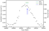 |
Fig. 1. Swift/BAT (15–50 keV) daily average light curve of EXO 2030+375 (black dots with gray error bars). Times of each continuous and pointed observations used in this work are marked by horizontal colored lines and vertical arrows, as detailed in the legend. |
2.2. SRG/ART-XC
The Mikhail Pavlinsky ART-XC telescope (Pavlinsky et al. 2021) carried out two consecutive observations (ObsIDs: 12210071001, 12210071002) of EXO 2030+375, from 2022 November 25–26 (MJD 59908.87–59909.62 and 59909.71–59909.83), simultaneously with IXPE, with a total net exposure of 75 ks. ART-XC is a grazing incidence-focusing X-ray telescope on board the SRG observatory (Sunyaev et al. 2021). The telescope includes seven independent modules and provides imaging, timing, and spectroscopy in the 4–30 keV energy range, with a total effective area of ∼450 cm2 at 6 keV, angular resolution of 45″, energy resolution of 1.4 keV at 6 keV, and timing resolution of 23 μs. The ART-XC data were processed with the software ARTPRODUCTS v1.0 and the CALDB version 20230228. We limited the ART-XC energy band to the 6.5–25 keV energy range, where the instrument calibration is better known. Following standard procedures, we merged data from both observations, rebinned the spectrum to match the energy resolution of the detectors, and added a systematic error of 2% to it.
2.3. Insight-HXMT
Hard X-ray Modulation Telescope (HXMT, also dubbed as Insight-HXMT) excels in its broad energy band (1–250 keV) and a large effective area in the hard X-ray energy band (Zhang et al. 2020). EXO 2030+375 was observed by HXMT from 2022 November 18 (MJD 59901) to November 27 (MJD 59910). In this work, we only analyze quasi-simultaneous observations with IXPE from 2022 November 23 (MJD 59905) to November 27 (MJD 59910). The resulting total exposure times are 42 ks, 71 ks and 67 ks for the detectors of three payloads on board HXMT, LE (1–15 keV), ME (5–30 keV), and HE (20–250 keV), respectively. The detectors were used to generate the events in good time intervals (GTIs). The time resolution of the HE, ME, and LE instruments are ∼25 μs, ∼280 μs, and ∼1 ms, respectively. Data from HXMT were considered in the range 2–70 keV, with the exclusion of 21–24 keV data due to the presence of an Ag feature (Li et al. 2020). Insight-HXMT Data Analysis software3 (HXMTDAS) v2.05 and HXMTCALDB v2.05 are used to analyze the data. We screened events for three payloads in HXMTDAS using legtigen, megtigen, hegtigen tasks according to the following criteria for the selection of GTIs: (1) pointing offset angle < 0.1°; (2) the elevation angle > 10°; (3) the geomagnetic cut-off rigidity > 8 GeV; (4) the time before and after the South Atlantic Anomaly passage > 300 s; (5) for LE observations, pointing direction above bright Earth > 30°. We selected events from the small field of views (FoVs) for LE and ME observations, and from both small and large FoVs for HE observations due to the limitation of the background calibration. The instrumental background is estimated by blocking the collimators of some detectors completely. The background model is developed by taking the correlations of the count rates between the blind and other detectors. The background is generated with lebkgmap, mebkgmap, and hebkgmap implemented in HXMTDAS, respectively. We restricted the energy band for spectral analysis to 1–10, 10–30, and 30–70 keV for LE, ME, and HE, respectively, as these ranges suffer smaller calibration uncertainties given the available observational background. Following the official team recommendations, we added a systematic error of 1% to LE and ME spectra, and 3% to the HE spectrum.
3. Data analysis and results
Polarimetric parameters were derived following the approach based on the formalism by Kislat et al. (2015), as implemented in the pcube software algorithm and through spectro-polarimetric analysis available in XSPEC (Strohmayer 2017). The spectra were fitted simultaneously in XSPEC allowing for a cross-calibration constant to account for calibration uncertainties of different DUs with respect to other detectors and for intrinsic source variability. The source spectra were rebinned to have at least 30 counts per energy channel in order to adopt the χ2 fit statistic, given the non-Poissonian nature of the source spectra. The adopted test statistic was the χ2. Spectral data were analyzed with XSPEC version 12.13.0b (Arnaud 1996) available with HEASOFT v6.31.
3.1. Timing analysis
Barycentric correction was applied to the events using the barycorr tool for IXPE and ART-XC, and the HXMTDAS task hxbary for HXMT. DE421 Solar system ephemeris and the SIMBAD (Wenger et al. 2000) ICRS coordinates of the source were employed to this aim. Binary demodulation also was performed, employing the orbital solution from Fu et al. (2023). The final estimate of the spin period Ps = 41.1187(1) s was then obtained using the phase connection technique (Deeter et al. 1981) and HXMT/LE events. The obtained spin period was used to fold the events from all employed instruments and obtain corresponding pulse profiles.
For completeness, we also extracted the IXPE light curve in the 2–8 keV energy band summed over the three DUs and rebinned at 300 s. The resulting light curve shows a steady count rate of about 5 cnt s−1 over the whole IXPE observation.
3.2. Phase-averaged analysis
3.2.1. Phase-averaged polarimetric analysis
Polarization quantities were initially derived following the model-independent approach described in Kislat et al. (2015) and Baldini et al. (2022). Normalized Stokes parameters, Q/I and U/I, were extracted using the pcube algorithm within IXPEOBSSIM and then used to obtain the PD and PA. Figure 2 shows those parameters for the full 2–8 keV energy band, while Fig. 3 shows the same in different energy bands. Both plots show that the normalized Stokes parameters are consistent with zero, which implies that the PD is also consistent with zero and is lower than ∼3% at 99% c.l.
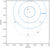 |
Fig. 2. Pulse phase-averaged normalized Stokes parameters U/I (y-axis) and Q/I (x-axis) over the 2–8 keV energy range. The 1σ, 2σ, and 3σ contours are plotted as concentric circles around the nominal value (continuous and dashed lines, respectively). The gray dotted circle represents loci of constant 1% PD, while radial lines are labeled for specific electric vector position angles (that is, the polarization angle, PA) with respect to north. The phase-averaged PD upper limit is about 2% at 99% c.l. |
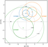 |
Fig. 3. Same details as in Fig. 2 for energy-dependent normalized Stokes parameters. Gray dotted circles represents loci of constant 1% and 2% PD. Blue, orange, and green circles represent the 2–4, 4–6 and 6–8 keV energy bands, respectively. |
3.2.2. Phase-averaged spectro-polarimetric analysis
To perform the spectro-polarimetric analysis, we first limited the study to IXPE data only. The I, Q, and U spectra from the source were extracted using the xpbin algorithm for each DU. Given the narrow energy range of IXPE data, the spectra can be fitted with a simpler model than that required for broader-band analysis. We therefore employed a simple absorbed power-law model for the IXPE-only analysis. A constant polarization component (energy-independent PD and PA) was also added to the model in XSPEC. The final form of the model was thus const×tbabs(powerlaw×polconst). This model returns a fit-statistic χ2/d.o.f. = 1372/1334 (see Table 1 and Fig. 4). Errors are calculated through MCMC simulations using the Goodman-Weare algorithm of length 2 × 10⁵ with 20 walkers and 104 burn-in steps. Best-fit results are shown in Table 1. The analysis reveals a PD of 1.2 ± 0.6% at the 90% c.l.
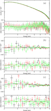 |
Fig. 4. EXO 2030+375 spectral energy distribution of the phase-averaged Stokes parameters I, Q, and U as observed by IXPE – panels (a), (b), and (c), respectively. Continuous lines in the top panels represent the best-fit model const×tbabs(powerlaw×polconst) reported in Table 1. Bottom panels show the residuals. Different colors represent different detectors – black for DU1, red for DU2, and green for DU3. Data have been rebinned and re-normalized for plotting purpose. |
Best-fit parameters of the phase-averaged IXPE data on EXO 2030+375 obtained from spectro-polarimetric analysis using model const×tbabs(powerlaw×polconst) in the 2–8 keV energy band.
To test a possible energy-dependence of the polarization properties in EXO 2030+375, different polarization model components were also tested, namely pollin and polpow in XSPEC, corresponding to a linear and a power-law dependence with energy, respectively, of the PD and PA. However, these models did not further reduce the χ2 value, nor returned significantly different polarimetric quantities and were, therefore, not explored further.
Finally, we simultaneously fitted IXPE, HXMT, and ART-XC spectra. In principle, with a broadband spectrum available, polarimetric results suffer less contamination from a possibly incorrect spectral model derived by the restricted IXPE energy band. Following previous works (Klochkov et al. 2008; Epili et al. 2017; Fürst et al. 2018; Tamang et al. 2022), we adopted an absorbed power-law model with high-energy cutoff and an iron Kα line. To this, we added a constant polarization component as above. As the iron line is produced by fluorescence, it is not expected to be polarized. We verified this by adding a separate polconst component for the continuum and for the iron line. This resulted in a best-fit model whose PD value for the iron line was pegged at its lower limit. Therefore, we left that component unaffected by polarization. The final model expression is thus const×tbabs(powerlaw×highecut×polconst+gauss). For the fitting procedure, IXPE and SRG/ART-XC spectral parameters were tied to those from HXMT/LE, leaving a cross-calibration constant free for each instrument. For the photoelectric absorption from neutral interstellar matter, we employed the tbabs model from Wilms et al. (2000) and relative wilm abundances. The Galactic column density in the direction of the source is about 8.8 × 1021 cm−2 (HI4PI Collaboration 2016).
Despite the more elaborate model (with respect to the IXPE-only analysis) and the broad 2–70 keV energy band, we were still able to verify that the obtained best-fit values of the PD and PA are in agreement with those reported in Sect. 3.2.1 within 1σ. The broadband spectral results are shown in Fig. 5 and reported in Table 2.
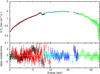 |
Fig. 5. Phase-averaged broadband spectrum of EXO 2030+375. Top: EXO 2030+375 unfolded EFE spectrum as observed by IXPE, HXMT, and ART-XC. For plotting purpose, data from the three IXPE DUs are combined and re-normalized, and all spectra are rebinned. IXPE data are in red, HXMT LE, ME, and HE in black, blue and green, respectively, ART-XC data are in cyan. Bottom: residuals of the best-fit model (also see Table 2). |
Best-fit parameters of the phase-averaged broadband spectrum of EXO 2030+375 as observed by IXPE, HXMT and ART-XC and obtained from spectro-polarimetric analysis using the model const×tbabs(powerlaw×highecut×polconst+gauss) in the 2–70 keV energy band.
3.3. Phase-resolved (spectro-)polarimetric analysis
To perform a phase-resolved polarization analysis of IXPE data, we selected seven phase bins to sample different flux levels shown by the pulse profile (see Fig. 6). The phase bins were extracted with respect to T0 = 59906.82181991 MJD.
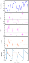 |
Fig. 6. Phase-resolved results of EXO 2030+375 in the 2–8 keV range, combining data from all IXPE DUs. From top to bottom, we show the pulse profile, normalized Stokes parameters q and u based on the polarimetric analysis, and the PD and PA, as obtained from the spectro-polarimetric analysis. The blue line in the PA panel corresponds to the best-fit rotating vector model (see Sect. 4.2). |
For the polarimetric analysis, we followed the Kislat et al. (2015) formalism as outlined in Sect. 3.2.1. The results, shown in Fig. 6, exhibit only a moderate variability of the Stokes parameters as a function of the pulse phase.
To perform the spectro-polarimetric analysis of the phase-resolved spectra, we used the same model as we did for the phase-averaged analysis in Sect. 3.2.2. Phase-resolved spectra were rebinned analogously to the phase-averaged analysis. For IXPE, cross-normalization constants were kept fixed at their correspondent phase-averaged value (see Table 1). The resulting best-fit values are reported in Table 3 and shown in Fig. 6. The analysis reveals significant detection of polarization up to about 7%. Both the PD and PA show pronounced variation with spin phase.
Best-fit results of the spectro-polarimetric analysis of the phase-resolved IXPE data of EXO 2030+375 using the const×tbabs(powerlaw×polconst) model in the 2–8 keV energy band.
3.4. Phase-resolved spectral analysis
Taking advantage of the long, broadband HXMT observations, we also performed a pulse phase-resolved spectral analysis of the HXMT data. For this, 11 phase bins were chosen to provide similar statistics of spectra in each bin. However, given the limited statistics with respect to phase-averaged analysis, we limited HXMT/HE data to 50 keV. To model the phase-resolved spectra, we used the same model employed for the phase-averaged spectrum (see Sect. 3.2.2). The best-fit results are reported in Fig. 7. The analysis shows strong variability of the spectral parameters with pulse phase. We notice that the observed parameter variations might at least partly due to artificial correlations of degenerate parameters. We tested this through the calculation of contour plots for different pairs of parameters and verified that although the parameters show some intrinsic correlations, their variability is still significant. Although part of this variability is known to be model-dependent (Klochkov et al. 2008; Hemphill et al. 2014), it is nonetheless useful to test luminosity-dependence of the parameters variability with pulse phase (see Sect. 4.3).
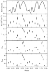 |
Fig. 7. Best-fit parameters for the broadband (2 − 50 keV) phase-resolved spectra of EXO 2030+375 as observed by HXMT. Panels from top to bottom show the pulse profile as observed by HXMT/LE in the 2–10 keV energy band; the column density, NH; the power-law photon index Γ; the cutoff energy; and the folding energy (both in keV). |
4. Discussion
4.1. Polarization degree: Expectations versus observations
Our analysis shows a low polarization for the X-ray radiation from EXO 2030+375, with the phase-averaged PD in the 0%–3% range and the phase-resolved PD values in the range of 2%–7%. High values for the PD were expected from theoretical models of accreting XRPs (Caiazzo & Heyl 2021b,a, and references therein). This is due to both plasma and vacuum birefringence, which modify the opacity in the magnetic field depending on polarization of photons. Thus, emitted photons get polarized in two normal modes, namely: ordinary (O) and extraordinary (X), representing oscillations of the electric field parallel and perpendicular to the plane formed by the local magnetic field and the photon momentum, respectively.
Recently, however, those models have been challenged by IXPE observations of several accreting XRPs, namely: Her X-1 (Doroshenko et al. 2022), Cen X-3 (Tsygankov et al. 2022), 4U 1626−67 (Marshall et al. 2022), Vela X-1 (Forsblom et al. 2023), and GRO J1008−57 (Tsygankov et al. 2023). In fact, all those sources show a far lower PD than expected. The observed relatively low polarization was interpreted in terms of a “vacuum resonance” occurring where the contributions from plasma and vacuum are equal (Lai & Ho 2002). Passing through the resonance, ordinary and extraordinary polarization modes of X-ray photons would convert to each other, with a net effect of depolarizing the radiation. This process takes place at a plasma density  g cm−3, where B12 is the magnetic field strength in units of 1012 G and EkeV is the photon energy in keV. Doroshenko et al. (2022) found that a transition layer of about 3 g cm−2 (corresponding to a Thomson optical depth of about unity) would depolarize the observed radiation consistently with the measured polarimetric quantities – if the vacuum resonance is located in the overheated atmospheric layer, which happens in the sub-critical (or low-) accretion regime. With the 2–10 keV flux of 2.5 × 10⁻⁹ erg cm−2 s−1 (see Table 1) and at a distance of 2.4 kpc, the observed source luminosity is 2 × 1036 erg s−1. This luminosity value is comparable to the low luminosity state of Cen X-3 (Tsygankov et al. 2022) and to the bright state of GRO J1008−57 (Tsygankov et al. 2023), as observed by IXPE. The former also shows no significant polarization in the phase-averaged analysis, while the latter shows significant polarization of about 4%. Therefore, it is possible that some other mechanisms beyond those linked to the accretion luminosity are responsible for the observed polarization degree.
One qualitative interpretation of the observed low PD is pointed by the complex pulse profile of EXO 2030+375 (see Figs. 6 and 7). Such a complexity may derive from a complex magnetic field geometry where different hot spots simultaneously contribute to the observed emission at different pulse phases. The observed low PD might therefore be interpreted as due to mixing of emission from several parts of NS surface observed at different angles.
Another interpretation can be linked to the relation between the magnetic field geometry, in particular, the magnetic obliquity and the observer’s line of sight. If the magnetic dipole is nearly aligned with the rotation axis and the observer looks from the side (as seems to be the case for Her X-1 and Cen X-3), the changes in the PA with the pulsar phase are rather small and the average polarization is significant. On the other hand, for a highly inclined dipole (especially when observed at small inclinations), the variations of the dipole position angle (that is reflected in the PA) are large, resulting in a strongly reduced average polarization. This interpretation is in line with the results obtained for the system geometry in EXO 2030+375 and further discussed in the next section.
4.2. Geometry of the system
The polarimetric quantity PA can be exploited to constrain the geometry of the system by fitting the unbinned polarimetric measurements from individual photoelectric angles with the rotating-vector model (RVM, Radhakrishnan & Cooke 1969; Poutanen 2020). If radiation escapes in the O-mode, the RVM describes the PA as follows:
 (1)
(1)
where ip is the pulsar inclination (the angle between the pulsar spin vector and the line of sight), χp is the position angle (measured from north to east) of the pulsar spin, θ is the magnetic obliquity (the angle between the magnetic dipole and the spin axis), ϕ is the pulse phase, and ϕ0 is the phase when the northern magnetic pole is closest to the observer. The other pole makes its closest approach half a period later. Using the RVM fit to the unbinned Stokes parameters on a photon-by-photon basis (González-Caniulef et al. 2023) and running Markov chain Monte Carlo (MCMC) simulations, we obtained estimates of the pulsar inclination, namely:  deg, along with the co-latitude of the magnetic pole (or magnetic obliquity),
  deg, and the position angle of the pulsar spin, χp = χp, O = −30 ± 5 deg (see Fig. 8). With the pulsar inclination and magnetic obliquity angles being almost supplementary, ip + θ ≈ 180°, the southern magnetic pole swings close to the observer line of sight at each pulsar rotation at half a period from phase ϕ0/(2π), that is: at
  .
.
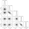 |
Fig. 8. Corner plot of the posterior distribution for the RVM parameters for the pulsar geometry obtained using the PA values. Parameters are the PD of radiation escaping from the magnetic pole, pulsar inclination, ip; magnetic obliquity, θ; position angle, χp; and the phase, ϕ0. 2D contours correspond to 68%, 95% and 99% confidence levels. The histograms show the normalized 1D distribution for a given parameter derived from the posterior samples. The mean value and 1σ confidence levels for the derived parameters are reported above the corresponding histogram. |
Interestingly, in the case of EXO 2030+375 the RVM suggests a relatively high magnetic obliquity. Other XRPs (e.g., Her X-1, Cen X-3) show θ ≈ 15°, while a value of θ ≈ 60° observed from EXO 2030+375 is closer to the orthogonal rotator GRO J1008−57 (Tsygankov et al. 2023). These results indicate that EXO 2030+375 stands in between the bimodal distribution peaking at 0° and 90° of the magnetic obliquity expected for isolated NSs (Dall’Osso & Perna 2017; Lander & Jones 2018), although such results do not necessarily apply to accreting XRPs (Biryukov & Abolmasov 2021).
The orbital inclination can be obtained from the orbital parameters measured by Wilson et al. (2008). For the optical companion stellar mass in the range 17–20 M⊙, corresponding to B0V spectral class (Coe et al. 1988), and assuming a NS mass of 1.4 M⊙, the inclination is in the range 49°–55° (see also Laplace et al. 2017). This value is consistent with the pulsar inclination value derived through the RVM fit because the sense of rotation cannot be determined from the X-ray pulse arrival times (i.e., solutions in the range iorb = 125°–131° are equally probable).
4.3. HXMT phase-resolved spectral results
Spectral parameters are expected to show pulse phase-dependence due to the highly anisotropic accretion geometry in XRPs. We therefore performed phase-resolved spectroscopy of HXMT EXO 2030+375 data (see Fig. 7). Phase-resolved spectroscopy of EXO 2030+375 was also performed in earlier works (Klochkov et al. 2008; Naik & Jaisawal 2015; Tamang et al. 2022). However, despite the main continuum model used in past works is similar to the one adopted here, several important differences prevent a direct comparison. In fact, XRP spectra are known to be luminosity-dependent (Mushtukov & Tsygankov 2022) and, as a consequence, different spectral components can be adopted to fit the data collected at different luminosity levels.
For EXO 2030+375, the main continuum model was modified in different works with additional components such as a Gaussian absorption line around 10 keV (Klochkov et al. 2008) or a partial covering component (Naik & Jaisawal 2015; Tamang et al. 2022). Therefore, only a qualitative comparison can be made between the results obtained here and those from previous works. For example, observations carried out by Klochkov et al. (2008) of EXO 2030+375 show that the power-law photon index reaches a minimum around the main pulse profile peak (corresponding to the broad main peak at ϕ ∼ 0.8 in Fig. 7). A similar trend has emerged also from the phase-resolved results observed in Her X-1 (Vasco et al. 2013). Here, in contrast, we observe a maximum value of the photon index around the same peak (see Fig. 7). This is likely a consequence of the luminosity difference, as the above-mentioned works derive their results in the high-luminosity accretion regime (1037 − 38 erg s−1, that is near or above the critical luminosity), whereas in the present work the source has been observed at sub-critical luminosity (∼4 × 1036 erg s−1). Such a difference is reflected in two main aspects. On the one side, the accretion structure beaming pattern is expected to drastically change at different regimes. In fact, the EXO 2030+375 pulse profile observed in the high-luminosity regime (see, e.g., the 2–9 keV panel in Fig. 2 of Klochkov et al. 2008) exhibits substantial differences with what is observed in the present work (see top panel in Fig. 7). This can lead to opposite observational signatures if the observer looks through the optically deep walls of the accretion column in the super-critical regime or through the optically thin hot-spots in the sub-critical regime (Mushtukov et al. 2015; Becker & Wolff 2022). On the other hand, opposite luminosity-dependences of spectral parameters have been observed in different accretion regimes in XRPs, depending on whether a gas-mediated or a radiation-dominated shock is responsible for the infalling plasma deceleration (Klochkov et al. 2011, and references therein). Although such behavior has generally been observed in the pulse-averaged analysis (see, e.g., Müller et al. 2013; Reig & Nespoli 2013; Malacaria et al. 2015; Diez et al. 2022), pulse-to-pulse spectroscopy hints at the possibility that similar trends are at work on shorter timescales (Klochkov et al. 2011; Vybornov et al. 2017; Müller et al. 2013) and that even phase-resolved spectroscopy exhibits a pulse-phase dependence of most parameters on luminosity (Lutovinov et al. 2016).
The system geometry derived in Sect. 4.2 shows that the southern magnetic pole swings close to the observer line of sight at phase 0.1 (that is, half a period from ϕ0). As the observation is carried out at sub-critical accretion, an accretion column with emitting walls contributing at neighbor phases is not expected. Thus, the main pulse profile peak at phase 0.8 is perhaps due to light bending from pencil beam emission at the magnetic poles. Such emission is generated in an optically thin environment at the hot-spot and it is therefore intrinsically soft, leading to a maximum of the photon index. However, this scenario would likely produce a symmetrical behavior of the spectral parameters dependence around the phase ϕ0, which is not observed here. This result, together with the highly-structured pulse profile, hints to a more complex NS configuration, such as a multipolar or asymmetric topology of the magnetic field. This kind of magnetic field configuration has also been recently proposed for other XRPs (Postnov et al. 2013; Tsygankov et al. 2017; Israel et al. 2017; Mönkkönen et al. 2022).
5. Summary
Our main results can be summarized as follows:
-
EXO 2030+375 was observed in November 2022 by IXPE, HXMT and ART-XC at the peak of a low-luminosity Type I outburst.
-
Only a low polarization degree of 0%–3% has been found in the phase-averaged analysis, while the phase-resolved analysis reveals a PD in the range of 2%–7%.
-
The observed low PD can be explained in terms of an overheated NS atmosphere scenario, with additional depolarizing mechanisms possibly at work in EXO 2030+375. We propose that mixing of emission from several parts of the NS surface observed at different angles, on one hand, and variations of the dipole position angle resulting in changes in the PA on the other, would lead to further depolarization.
-
By means of the rotating vector model, we constrained the geometry of the accreting pulsar. The pulsar inclination is ∼130°, almost supplementary to the magnetic obliquity angle, at ∼60° (that is, their sum is ∼180°). The obtained pulsar geometry implies that the magnetic axis swings close to the observer line of sight and the system obliquity stands between orthogonal and aligned rotators.
-
The spectral phase-resolved analysis shows evidence that the pulse phase dependence of spectral parameters is different for different luminosities. This possibly reflects changes in the accretion structure at different accretion regimes, accompanied by beam pattern changes.
-
Polarimetric, spectral, and timing analyses all hint toward a complex accretion geometry, where magnetic multipoles with asymmetric topology and gravitational light bending have significant effects on the resulting spectral and timing behavior of EXO 2030+375.
Our analysis of EXO 2030+375 characterized the X-ray polarimetric and spectral properties of the source at the sub-critical accretion regime. Additional future observations at different luminosities would help discerning the various mechanisms at work that shape the X-ray emission properties.
Acknowledgments
The Imaging X-ray Polarimetry Explorer (IXPE) is a joint US and Italian mission. The US contribution is supported by the National Aeronautics and Space Administration (NASA) and led and managed by its Marshall Space Flight Center (MSFC) with industry partner Ball Aerospace (contract NNM15AA18C). The Italian contribution is supported by the Italian Space Agency (Agenzia Spaziale Italiana, ASI) through contract ASI-OHBI-2017-12-I.0, agreements ASI-INAF-2017-12-H0 and ASI-INFN-2017.13-H0, and its Space Science Data Center (SSDC) with agreements ASI-INAF-2022-14-HH.0 and ASI-INFN 2021-43-HH.0, and by the Istituto Nazionale di Astrofisica (INAF) and the Istituto Nazionale di Fisica Nucleare (INFN) in Italy. This research used data products provided by the IXPE Team (MSFC, SSDC, INAF, and INFN) and distributed with additional software tools by the High-Energy Astrophysics Science Archive Research Center (HEASARC), which is a service of the Astrophysics Science Division at NASA/GSFC and the High Energy Astrophysics Division of the Smithsonian Astrophysical Observatory. We acknowledge extensive use of the NASA Abstract Database Service (ADS). This research was supported by the International Space Science Institute (ISSI) in Bern, through ISSI International Team project 495. JH acknowledges support from the Natural Sciences and Engineering Research Council of Canada (NSERC) through a Discovery Grant, the Canadian Space Agency through the co-investigator grant program, and computational resources and services provided by Compute Canada, Advanced Research Computing at the University of British Columbia, and the SciServer science platform (www.sciserver.org). We also acknowledge support from the Academy of Finland grants 333112, 349144, 349373, and 349906 (SST, JP), the German Academic Exchange Service (DAAD) travel grant 57525212 (VD, VFS), the Väisälä Foundation (SST), the Russian Science Foundation grant 19-12-00423 (AAL, IAM, SVM, AES), the French National Centre for Scientific Research (CNRS), and the French National Centre for Space Studies (CNES) (POP). We thank Lingda Kong and Youli Tuo for their helpful assistance in the HXMT data analysis.
References
- Arnaud, K. A. 1996, in Astronomical Data Analysis Software and Systems V, eds. G. H. Jacoby, & J. Barnes (San Francisco: ASP), ASP Conf. Ser., 101, 17 [NASA ADS] [Google Scholar]
- Bailer-Jones, C. A. L., Rybizki, J., Fouesneau, M., Demleitner, M., & Andrae, R. 2021, AJ, 161, 147 [Google Scholar]
- Baldini, L., Barbanera, M., Bellazzini, R., et al. 2021, Astropart. Phys., 133, 102628 [NASA ADS] [CrossRef] [Google Scholar]
- Baldini, L., Bucciantini, N., Lalla, N. D., et al. 2022, SoftwareX, 19, 101194 [NASA ADS] [CrossRef] [Google Scholar]
- Becker, P. A., & Wolff, M. T. 2022, ApJ, 939, 67 [NASA ADS] [CrossRef] [Google Scholar]
- Bellazzini, R., & Angelini, F. 2003, in Polarimetry in Astronomy, ed. S. Fineschi, Proc. SPIE, 4843, 383 [NASA ADS] [CrossRef] [Google Scholar]
- Biryukov, A., & Abolmasov, P. 2021, MNRAS, 505, 1775 [NASA ADS] [CrossRef] [Google Scholar]
- Caiazzo, I., & Heyl, J. 2021a, MNRAS, 501, 129 [Google Scholar]
- Caiazzo, I., & Heyl, J. 2021b, MNRAS, 501, 109 [Google Scholar]
- Coe, M. J., Longmore, A., Payne, B. J., & Hanson, C. G. 1988, MNRAS, 232, 865 [NASA ADS] [CrossRef] [Google Scholar]
- Corbet, R. H. D., & Levine, A. M. 2006, ATel, 843, 1 [NASA ADS] [Google Scholar]
- Dall’Osso, S., & Perna, R. 2017, MNRAS, 472, 2142 [Google Scholar]
- Deeter, J. E., Boynton, P. E., & Pravdo, S. H. 1981, ApJ, 247, 1003 [NASA ADS] [CrossRef] [Google Scholar]
- Diez, C. M., Grinberg, V., Fürst, F., et al. 2022, A&A, 660, A19 [NASA ADS] [CrossRef] [EDP Sciences] [Google Scholar]
- Di Marco, A., Costa, E., Muleri, F., et al. 2022, AJ, 163, 170 [NASA ADS] [CrossRef] [Google Scholar]
- Di Marco, A., Soffitta, P., Costa, E., et al. 2023, AJ, 165, 143 [CrossRef] [Google Scholar]
- Doroshenko, V., Poutanen, J., Tsygankov, S. S., et al. 2022, Nat. Astron., 6, 1433 [NASA ADS] [CrossRef] [Google Scholar]
- Epili, P., Naik, S., Jaisawal, G. K., & Gupta, S. 2017, MNRAS, 472, 3455 [CrossRef] [Google Scholar]
- Forsblom, S. V., Poutanen, J., Tsygankov, S. S., et al. 2023, ApJ, 947, L20 [NASA ADS] [CrossRef] [Google Scholar]
- Fu, Y.-C., Song, L. M., Ding, G. Q., et al. 2023, MNRAS, 521, 893 [CrossRef] [Google Scholar]
- Fürst, F., Falkner, S., Marcu-Cheatham, D., et al. 2018, A&A, 620, A153 [NASA ADS] [CrossRef] [EDP Sciences] [Google Scholar]
- Gehrels, N., Chincarini, G., Giommi, P., et al. 2004, ApJ, 611, 1005 [Google Scholar]
- Gnedin, Y. N., Pavlov, G. G., & Shibanov, Y. A. 1978, Sov. Astron. Lett., 4, 117 [Google Scholar]
- González-Caniulef, D., Caiazzo, I., & Heyl, J. 2023, MNRAS, 519, 5902 [CrossRef] [Google Scholar]
- Hemphill, P. B., Rothschild, R. E., Markowitz, A., et al. 2014, ApJ, 792, 14 [NASA ADS] [CrossRef] [Google Scholar]
- HI4PI Collaboration (Ben Bekhti, N., et al.) 2016, A&A, 594, A116 [NASA ADS] [CrossRef] [EDP Sciences] [Google Scholar]
- Israel, G. L., Belfiore, A., Stella, L., et al. 2017, Science, 355, 817 [NASA ADS] [CrossRef] [Google Scholar]
- Kislat, F., Clark, B., Beilicke, M., & Krawczynski, H. 2015, Astropart. Phys., 68, 45 [NASA ADS] [CrossRef] [Google Scholar]
- Klochkov, D., Santangelo, A., Staubert, R., & Ferrigno, C. 2008, A&A, 491, 833 [NASA ADS] [CrossRef] [EDP Sciences] [Google Scholar]
- Klochkov, D., Staubert, R., Santangelo, A., Rothschild, R. E., & Ferrigno, C. 2011, A&A, 532, A126 [NASA ADS] [CrossRef] [EDP Sciences] [Google Scholar]
- Krimm, H. A., Holland, S. T., Corbet, R. H. D., et al. 2013, ApJS, 209, 14 [NASA ADS] [CrossRef] [Google Scholar]
- Lai, D., & Ho, W. C. G. 2002, ApJ, 566, 373 [NASA ADS] [CrossRef] [Google Scholar]
- Lander, S. K., & Jones, D. I. 2018, MNRAS, 481, 4169 [NASA ADS] [CrossRef] [Google Scholar]
- Laplace, E., Mihara, T., Moritani, Y., et al. 2017, A&A, 597, A124 [NASA ADS] [CrossRef] [EDP Sciences] [Google Scholar]
- Li, X., Li, X., Tan, Y., et al. 2020, J. High Energy Astrophys., 27, 64 [NASA ADS] [CrossRef] [Google Scholar]
- Lutovinov, A. A., Buckley, D. A. H., Townsend, L. J., Tsygankov, S. S., & Kennea, J. 2016, MNRAS, 462, 3823 [NASA ADS] [CrossRef] [Google Scholar]
- Malacaria, C., Klochkov, D., Santangelo, A., & Staubert, R. 2015, A&A, 581, A121 [NASA ADS] [CrossRef] [EDP Sciences] [Google Scholar]
- Marshall, H. L., Ng, M., Rogantini, D., et al. 2022, ApJ, 940, 70 [NASA ADS] [CrossRef] [Google Scholar]
- Meszaros, P., Novick, R., Szentgyorgyi, A., Chanan, G. A., & Weisskopf, M. C. 1988, ApJ, 324, 1056 [NASA ADS] [CrossRef] [Google Scholar]
- Mönkkönen, J., Tsygankov, S. S., Mushtukov, A. A., et al. 2022, MNRAS, 515, 571 [CrossRef] [Google Scholar]
- Müller, D., Klochkov, D., Caballero, I., & Santangelo, A. 2013, A&A, 552, A81 [NASA ADS] [CrossRef] [EDP Sciences] [Google Scholar]
- Mushtukov, A., & Tsygankov, S. 2022, in Handbook of X-ray and Gamma-ray Astrophysics, eds. C. Bambi, & A. Santangelo (Singapore: Springer) [Google Scholar]
- Mushtukov, A. A., Suleimanov, V. F., Tsygankov, S. S., & Poutanen, J. 2015, MNRAS, 447, 1847 [NASA ADS] [CrossRef] [Google Scholar]
- Naik, S., & Jaisawal, G. K. 2015, RAA, 15, 537 [NASA ADS] [Google Scholar]
- Parmar, A. N., White, N. E., Stella, L., Izzo, C., & Ferri, P. 1989, ApJ, 338, 359 [NASA ADS] [CrossRef] [Google Scholar]
- Pavlinsky, M., Tkachenko, A., Levin, V., et al. 2021, A&A, 650, A42 [EDP Sciences] [Google Scholar]
- Pavlov, G. G., & Shibanov, Y. A. 1979, Sov. J. Exp. Theoret. Phys., 49, 741 [NASA ADS] [Google Scholar]
- Postnov, K., Shakura, N., Staubert, R., et al. 2013, MNRAS, 435, 1147 [CrossRef] [Google Scholar]
- Poutanen, J. 2020, A&A, 641, A166 [NASA ADS] [CrossRef] [EDP Sciences] [Google Scholar]
- Radhakrishnan, V., & Cooke, D. J. 1969, ApJ, 3, 225 [Google Scholar]
- Reig, P., & Coe, M. J. 1998, MNRAS, 294, 118 [NASA ADS] [CrossRef] [Google Scholar]
- Reig, P., & Nespoli, E. 2013, A&A, 551, A1 [NASA ADS] [CrossRef] [EDP Sciences] [Google Scholar]
- Silvestri, S., & IXPE Collaboration 2023, Nucl. Instrum. Methods Phys. Res. A, 1048, 167938 [CrossRef] [Google Scholar]
- Soffitta, P., Baldini, L., Bellazzini, R., et al. 2021, AJ, 162, 208 [CrossRef] [Google Scholar]
- Strohmayer, T. E. 2017, ApJ, 838, 72 [NASA ADS] [CrossRef] [Google Scholar]
- Sunyaev, R., Arefiev, V., Babyshkin, V., et al. 2021, A&A, 656, A132 [NASA ADS] [CrossRef] [EDP Sciences] [Google Scholar]
- Tamang, R., Ghising, M., Tobrej, M., Rai, B., & Paul, B. C. 2022, MNRAS, 515, 5407 [CrossRef] [Google Scholar]
- Thalhammer, P., Ballhausen, R., Pottschmidt, K., et al. 2021, ATel, 14911, 1 [NASA ADS] [Google Scholar]
- Tsygankov, S. S., Doroshenko, V., Lutovinov, A. A., Mushtukov, A. A., & Poutanen, J. 2017, A&A, 605, A39 [NASA ADS] [CrossRef] [EDP Sciences] [Google Scholar]
- Tsygankov, S. S., Doroshenko, V., Poutanen, J., et al. 2022, ApJ, 941, L14 [NASA ADS] [CrossRef] [Google Scholar]
- Tsygankov, S. S., Doroshenko, V., Mushtukov, A. A., et al. 2023, A&A, in press https://doi.org/10.1051/0004-6361/202346134 [Google Scholar]
- Vasco, D., Staubert, R., Klochkov, D., et al. 2013, A&A, 550, A111 [NASA ADS] [CrossRef] [EDP Sciences] [Google Scholar]
- Vybornov, V., Klochkov, D., Gornostaev, M., et al. 2017, A&A, 601, A126 [NASA ADS] [CrossRef] [EDP Sciences] [Google Scholar]
- Weisskopf, M. C., Soffitta, P., Baldini, L., et al. 2022, JATIS, 8, 026002 [NASA ADS] [Google Scholar]
- Wenger, M., Ochsenbein, F., Egret, D., et al. 2000, A&AS, 143, 9 [NASA ADS] [CrossRef] [EDP Sciences] [Google Scholar]
- Wilms, J., Allen, A., & McCray, R. 2000, ApJ, 542, 914 [Google Scholar]
- Wilson, C. A., Finger, M. H., & Camero-Arranz, A. 2008, ApJ, 678, 1263 [NASA ADS] [CrossRef] [Google Scholar]
- Zhang, S.-N., Li, T., Lu, F., et al. 2020, Sci. China Phys. Mech. Astron., 63, 249502 [NASA ADS] [CrossRef] [Google Scholar]
All Tables
Best-fit parameters of the phase-averaged IXPE data on EXO 2030+375 obtained from spectro-polarimetric analysis using model const×tbabs(powerlaw×polconst) in the 2–8 keV energy band.
Best-fit parameters of the phase-averaged broadband spectrum of EXO 2030+375 as observed by IXPE, HXMT and ART-XC and obtained from spectro-polarimetric analysis using the model const×tbabs(powerlaw×highecut×polconst+gauss) in the 2–70 keV energy band.
Best-fit results of the spectro-polarimetric analysis of the phase-resolved IXPE data of EXO 2030+375 using the const×tbabs(powerlaw×polconst) model in the 2–8 keV energy band.
All Figures
|
Fig. 1. Swift/BAT (15–50 keV) daily average light curve of EXO 2030+375 (black dots with gray error bars). Times of each continuous and pointed observations used in this work are marked by horizontal colored lines and vertical arrows, as detailed in the legend. |
| In the text | |
|
Fig. 2. Pulse phase-averaged normalized Stokes parameters U/I (y-axis) and Q/I (x-axis) over the 2–8 keV energy range. The 1σ, 2σ, and 3σ contours are plotted as concentric circles around the nominal value (continuous and dashed lines, respectively). The gray dotted circle represents loci of constant 1% PD, while radial lines are labeled for specific electric vector position angles (that is, the polarization angle, PA) with respect to north. The phase-averaged PD upper limit is about 2% at 99% c.l. |
| In the text | |
|
Fig. 3. Same details as in Fig. 2 for energy-dependent normalized Stokes parameters. Gray dotted circles represents loci of constant 1% and 2% PD. Blue, orange, and green circles represent the 2–4, 4–6 and 6–8 keV energy bands, respectively. |
| In the text | |
|
Fig. 4. EXO 2030+375 spectral energy distribution of the phase-averaged Stokes parameters I, Q, and U as observed by IXPE – panels (a), (b), and (c), respectively. Continuous lines in the top panels represent the best-fit model const×tbabs(powerlaw×polconst) reported in Table 1. Bottom panels show the residuals. Different colors represent different detectors – black for DU1, red for DU2, and green for DU3. Data have been rebinned and re-normalized for plotting purpose. |
| In the text | |
|
Fig. 5. Phase-averaged broadband spectrum of EXO 2030+375. Top: EXO 2030+375 unfolded EFE spectrum as observed by IXPE, HXMT, and ART-XC. For plotting purpose, data from the three IXPE DUs are combined and re-normalized, and all spectra are rebinned. IXPE data are in red, HXMT LE, ME, and HE in black, blue and green, respectively, ART-XC data are in cyan. Bottom: residuals of the best-fit model (also see Table 2). |
| In the text | |
|
Fig. 6. Phase-resolved results of EXO 2030+375 in the 2–8 keV range, combining data from all IXPE DUs. From top to bottom, we show the pulse profile, normalized Stokes parameters q and u based on the polarimetric analysis, and the PD and PA, as obtained from the spectro-polarimetric analysis. The blue line in the PA panel corresponds to the best-fit rotating vector model (see Sect. 4.2). |
| In the text | |
|
Fig. 7. Best-fit parameters for the broadband (2 − 50 keV) phase-resolved spectra of EXO 2030+375 as observed by HXMT. Panels from top to bottom show the pulse profile as observed by HXMT/LE in the 2–10 keV energy band; the column density, NH; the power-law photon index Γ; the cutoff energy; and the folding energy (both in keV). |
| In the text | |
|
Fig. 8. Corner plot of the posterior distribution for the RVM parameters for the pulsar geometry obtained using the PA values. Parameters are the PD of radiation escaping from the magnetic pole, pulsar inclination, ip; magnetic obliquity, θ; position angle, χp; and the phase, ϕ0. 2D contours correspond to 68%, 95% and 99% confidence levels. The histograms show the normalized 1D distribution for a given parameter derived from the posterior samples. The mean value and 1σ confidence levels for the derived parameters are reported above the corresponding histogram. |
| In the text | |
Current usage metrics show cumulative count of Article Views (full-text article views including HTML views, PDF and ePub downloads, according to the available data) and Abstracts Views on Vision4Press platform.
Data correspond to usage on the plateform after 2015. The current usage metrics is available 48-96 hours after online publication and is updated daily on week days.
Initial download of the metrics may take a while.