| Issue |
A&A
Volume 696, April 2025
|
|
|---|---|---|
| Article Number | L13 | |
| Number of page(s) | 11 | |
| Section | Letters to the Editor | |
| DOI | https://doi.org/10.1051/0004-6361/202553667 | |
| Published online | 15 April 2025 | |
Letter to the Editor
Water-cooled (sub)-Neptunes get better gas mileage
1
Faculty of Science, Tohoku University, Sendai, Miyagi 980-8578, Japan
2
Department of Earth Sciences, University of Hawai’i at Mänoa, Honolulu, Hawai’i 96822, USA
3
Institute for Astrophysics, University of Vienna, 1180 Vienna, Austria
⋆ Corresponding authors; This email address is being protected from spambots. You need JavaScript enabled to view it.
, This email address is being protected from spambots. You need JavaScript enabled to view it.
Received:
3
January
2025
Accepted:
26
March
2025
Abstract
The demographics of sub-Jovian planets around low-mass stars is dominated by populations of sub-Neptunes and super-Earths, distinguished by the presence or absence of envelopes of volatiles with a low molecular weight, that is, H2, He, and H2O. The current paradigm is that sub-Neptunes on close-in orbits evolve into super-Earths via atmospheric escape driven by high-energy stellar irradiation. We used an integrated hydrodynamic-radiation-chemical network model of the outflow to demonstrate that this escape is modulated by the abundance of H2O, which is an efficient infrared coolant. Increasing the H2O/H2 at the base of the flow induces a 1 dex decline in the escape rate, with definitive consequences for the retention of envelopes over Gyr. We show that saturation limits on H2O in the upper atmospheres of temperate sub-Neptunes could explain the paradoxical observation that these objects disappear more rapidly than their counterparts closer to their host stars. We also propose that the scarcity of sub-Neptunes around very low-mass stars could be related to the water-poor chemistry of their antecedent protoplanetary disks. Observations of atmospheric H2O by JWST as well as searches for atmospheric escape from younger planets using H and He lines could test these predictions.
Key words: planets and satellites: atmospheres
© The Authors 2025
 Open Access article, published by EDP Sciences, under the terms of the Creative Commons Attribution License (https://creativecommons.org/licenses/by/4.0), which permits unrestricted use, distribution, and reproduction in any medium, provided the original work is properly cited.
This article is published in open access under the Subscribe to Open model. This email address is being protected from spambots. You need JavaScript enabled to view it. to support open access publication.
1. Introduction
A photometric survey for transiting exoplanets by Kepler showed that Earth- to Neptune-size planets are far more numerous on close-in orbits around solar-type stars than Jovian counterparts (Howard et al. 2012; Petigura et al. 2013). The spectroscopic refinement of the host star (and hence, of the transiting planet) radii confirmed that this population consists of distinct super-Earth and sub-Neptune moieties with modal radii of about 1.3 and 2.2R⊕ that are separated by a sparsely populated valley at ∼1.7R⊕ (Owen & Wu 2013; Fulton et al. 2017; Petigura et al. 2022). This distribution appears to be universal among low-mass stars including M dwarfs (Cloutier & Menou 2020; Hirano et al. 2021; Venturini et al. 2024; Gaidos et al. 2024).
Planets much larger than the Earth but smaller than Neptune have no Solar System analog. Their formation, composition, and evolution are active areas of investigation in exoplanet research. Available combinations of the mass and radius measurements indicate that super-Earths are primarily rocky while sub-Neptunes have thick, low-density envelopes that are comprised of molecules with a low molecular weight, particularly H2, He, or H2O, around a rocky/icy core (Weiss & Marcy 2014). In the current paradigm, sub-Neptunes can lose their envelopes and evolve into super-Earths, and there is at least tentative evidence for atmospheric escape from some objects (e.g., Gaidos et al. 2022; Zhang et al. 2023; Rockcliffe et al. 2023; Orell-Miquel et al. 2023; Masson et al. 2024).
Photoevaporation of a planetary atmosphere occurs when its upper layers are heated to the energies required for escape by stellar extreme ultraviolet (EUV) radiation1. Under a sufficiently high irradiation, a collisional hydrodynamic flow can develop. The temperature profile in this flow is governed by the balance between absorption of stellar EUV radiation versus work done by the outflow, plus radiative cooling by atmospheric components. Radiative cooling is usually inefficient because absorption of X-rays and EUV invariably occurs above the homopause (or turbopause), where eddy diffusion can transport molecules against gravitational segregation. On Earth, the most important coolant molecules are CO2 and, more variably, nitric oxide (NO, Kockarts 1980). High levels of CO2 in the Archaean terrestrial atmosphere would have caused dramatically lower upper atmosphere temperatures relative to the present, suppressing escape (Johnstone et al. 2018). The recent anthropogenic increase in CO2 has caused a small but measurable decline in the temperatures in the mesosphere/lower thermosphere (Roble & Dickinson 1989; Mlynczak et al. 2022).
H2O has a lower molecular weight and is a more effective IR radiator than either CO2 or NO, but on Earth, with an equilibrium temperature Te ≈ 255 K, H2O is trapped in oceans and by condensation at altitudes ≲15 km, which is far below the homopause at 90 km. On planets with higher equilibrium temperatures, especially those in a runaway greenhouse state, H2O is entirely in the atmosphere (Kasting 1988) and the Clausius-Clapeyron relation permits higher H2O in the upper atmosphere. In sub-Neptunes with envelopes of H2-He, super-runaway irradiation means that interior H2O is in a supercritical phase that could be miscible with H2, allowing it to mix throughout the convective atmosphere (Pierrehumbert 2023). Planets with inflated steam-dominated atmospheres could be present in or even dominate the small-planet population on close-in orbits (Turbet et al. 2020; Piaulet-Ghorayeb et al. 2024). On the other hand, some planets may have accreted from oxygen-poor, dehydrated material and may lack H2 altogether (Gaidos 2000; Raymond et al. 2007).
The effect of variation in the H2O abundance on atmospheric escape rates and the evolution of small planets, particularly sub-Neptunes, has not yet been investigated. These effects could be observed around M dwarfs, where the orbital distance corresponding to water condensation falls within the limits of planet detection surveys. Here, we use a model of EUV-driven outflow to demonstrate this effect for temperate sub-Neptunes around M dwarfs, and we investigate how it can explain some aspects of exoplanet demographics.
2. Model
We used a radially symmetric 1D model of hydrodynamic escape (Yoshida & Kuramoto 2020; Yoshida et al. 2022), modified for an application to sub-Neptunes on close-in orbits around M-dwarf stars. Details of the model can be found in Appendix D. Here we outline the model briefly and focus on the modifications. We calculated atmospheric escape rates on a coarse 4D grid with respect to the stellar EUV flux, to the planetary gravitational acceleration g, to the H2O/H2 ratio at the base of the flow, and to the planetary mass. Using these rates, we evolved sub-Neptunes with a fixed planetary mass Mp and on circular orbits around an M2-type (0.45 M⊙) star, accounting for the (pre-main-sequence) evolution in stellar bolometric luminosity, and for the evolution in stellar EUV luminosity due to rotational spin-down. We adopted an Mp of 2.5 and 5M⊕, initial envelope mass fractions of 1–5%, and semi-major axes of 0.01–0.3 au, corresponding to main-sequence stellar irradiance of 0.3–250 times the current terrestrial value. The effect of fixing Mp in the evolutionary calculations was very weak because the atmospheric mass fraction is small. The planetary radius Rp was calculated as a function of the envelope mass fraction, age, and stellar irradiance using the models of Lopez & Fortney (2014). At each time-step, the H and O escape rates were calculated by interpolation on the grid, and the envelope mass fraction was adjusted accordingly. To calculate the atmospheric evolution, we fixed the basal H2O/H2 ratio, but we investigated the effect of allowing it to increase as a result of H escape in a single, fiducial case.
The atmosphere below the base of the outflow was assumed to be composed of H2 and H2O. Helium and other carbon- and nitrogen-bearing species were neglected. The lower and upper boundaries of the model were set at radial distances of Rp and 50Rp, respectively. The number density of H2 at the lower boundary was set at 1 × 1013 cm−3, which we assumed as the typical gas density at the altitude where stellar EUV irradiation is fully absorbed. The H2O/H2 ratio was fixed between 0 and 0.1 in each simulation. This is not equal to the H2O/H2 ratio in the deep atmosphere, that is, at or below the turbopause, where eddy diffusivity mixes the atmosphere constituents, but is instead a lower limit (see the discussion). The temperature at the lower boundary was set to the atmospheric skin temperature, which is the asymptotic temperature at high altitudes of the upper atmosphere that is optically thin in the thermal-IR and transparent to short-wave radiation (Catling & Kasting 2017). This basal temperature is 400 K at ∼10× the current terrestrial irradiance. Although this temperature depends on the semimajor axis, its variation affects the outflow structure and escape rate very little when the escape parameter, the ratio of the planetary gravitational potential energy to the thermal energy, exceeds ∼10 (Kubyshkina et al. 2018), as is the case here.
The governing equations in the model are the fluid equations of continuity, momentum, and energy for a multicomponent gas, plus those describing chemical reactions and radiative transport, assuming a spherically symmetric geometry. These equations were solved through time-dependent numerical integration until the physical quantities converged to steady profiles, following the calculation method in Yoshida & Kuramoto (2020). The chemical species and reactions we considered were the same as in Yoshida et al. (2022). We included 93 chemical reactions involving 15 species (H2, H2O, H, O, O(1D), OH, O2, H+, H , H
, H , O+, O
 , OH+, H2O+, and H3O+, Tables D.1 and D.2).
Heating by absorption of stellar X-rays and UV radiation was calculated using a reconstruction of the 0.1–280 nm spectrum of GJ 832 as a representative M2 dwarf (Loyd et al. 2016). The EUV flux at 1 au is 1.1 × 10⁻³ W m−2, about 25% that of the Sun. For the stellar EUV luminosity evolution, we adopted the model of Johnstone et al. (2021) for a star with a mass of 0.4M⊙ and an initial rotation rate ten times that of the current solar value. To represent both the higher EUV luminosity typical of young stars and a range of semimajor axes, we scaled this spectrum up to 104 times the current terrestrial irradiance. Heating and photolysis rate profiles were calculated by numerically solving the radiative transfer of parallel stellar photon beams in a spherically symmetric atmosphere, following the method of Tian et al. (2005). The resulting 3D heating distribution was averaged over spherical shells. Stellar visible and IR radiation was neglected as a heat source in the upper atmosphere. We included radiative cooling by thermal line emission from H2O, OH, H , OH+, and H3O+, using line data from the HITRAN (Rothman et al. 2013) and ExoMol (Tennyson et al. 2016) databases. In addition to the line emission considered by Yoshida et al. (2022), we included thermal line emission from H3O+ and expanded the line data for H2O and OH to cover a broader temperature range (Appendix D). We calculated radiative cooling rates for these species using the method formulated by Yoshida & Kuramoto (2020).
3. Results
3.1. Effect of the H2O abundance on escape rates
The escape rate Ṁ decreases with increasing basal H2O/H2 ratio due to enhanced radiative cooling and lower temperatures, regardless of gravity or EUV irradiance, with a 1 dex decrease at a basal H2O/H2 ratio of 0.1 relative to a pure H2 atmosphere (Fig. 1). This reduction in escape rate asymptotes at high H2O/H2 as the outflow becomes optically thick to IR radiation and H2O photolysis occurs deeper in the outflow because advection is slower. At a given basal H2O/H2 ratio, the escape rate is approximately proportional to FEUV, and it decreases with increasing g approximately as g−3/2, following the expected scaling for energy-limited escape (e.g., Owen 2019). Detailed atmospheric profiles are shown in Appendix A. The escape rate as a function of H2O/H2 ratio, FEUV, g, and Mp can be approximated by the following relation:
 (1)
(1)
![Mathematical equation: $$ \begin{aligned} \mathrm{log} _{10}\dot{M}_{\rm ref}\,[\mathrm M_{\oplus }/Gyr ]&=0.01042(\mathrm{log} _{10}r)^{3}+0.1257(\mathrm{log} _{10}r)^{2} \nonumber \\&+0.2429\mathrm{log} _{10}r-1.311, \end{aligned} $$](/articles/aa/full_html/2025/04/aa53667-25/aa53667-25-eq6.gif) (2)
(2)
 (3)
(3)
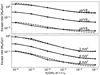 |
Fig. 1. Total escape rate vs. H2O/H2 for different values of EUV irradiance at fixed surface gravity g = 4 m s−2 (top panel) and for different values of g at a fixed EUV irradiance of 103F⊕ (bottom panel). Mp is fixed at 5M⊕. The dashed lines are from Eqs. (1)–(3). |
where  is the EUV flux at Earth, and r is the basal H2O/H2 ratio. aEUV decreases with increasing FEUV because as the temperature increases, radiative cooling becomes more effective (Yoshida & Kuramoto 2021). This function may become invalid under thermally instable conditions (Kubyshkina et al. 2018), extremely high EUV flux, and deep gravitational potential conditions such as those of hot Jupiters where atomic cooling is effective (Murray-Clay et al. 2009; Salz et al. 2016), and in the diffusion-limited regime (Hunten 1973).
3.2. H2O/H2-dependent evolution of sub-Neptunes
Figure 2 shows the evolutionary tracks of atmospheres with different H2O/H2 ratios for Mp = 2.5 M⊕ and a 1% initial envelope mass fraction, on an orbit where the main-sequence stellar flux is equivalent to the solar constant. High H2O/H2 ratios extend atmospheric lifetimes by reducing escape rates through radiative cooling (Fig. 2b). For H2O/H2 ratios above 10−3, envelopes persist for at least 10 Gyr, whereas atmospheres with lower H2O/H2 ratios are lost within the period (Fig. 2c). When mass fractionation between H and O is included (Appendix B), the atmospheric lifetimes slightly increase as the H2O/H2 ratio increases (dashed lines in Fig. 2c). Planets that retain significant envelopes have radii ≳2R⊕ (Fig. 2d).
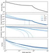 |
Fig. 2. Evolution of the EUV flux (top panel, a), escape rate (b), envelope mass (c), and planet radius (d) for a planet with Mp = 2.5M⊕, an initial envelope mass fraction of 1%, and different initial values of H2O/H2 on an orbit with a main-sequence stellar irradiance equal to the terrestrial value. The solid (dashed) lines represent results without (with) mass fractionation between H and O. The mass fractionation results are omitted from panel b for clarity. |
Figure 3 shows the envelope lifetime as a function of stellar irradiance and the H2O/H2 ratio, where the lifetime is defined as the time at which the atmospheric mass falls below 10−4Mp. The three scenarios in Fig. 2 with H2O/H2 > 0 are plotted as stars. The timescale increases with H2O/H2 and decreases with irradiance. The lifetime is weakly dependent on the initial envelope mass because gravity depends on the planetary radius, and hence, on the envelope mass (Fig. C1).
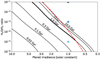 |
Fig. 3. Lifetime of envelopes with initial mass fraction of 1% on Mp = 2.5M⊕ sub-Neptunes as a function of stellar irradiance and H2O/H2. The dashed line is the saturation-limited H2O/H2 ratio in the upper atmosphere (see text and Appendix C). The stars represent the scenarios in Fig. 2. |
4. Discussion
Around low-luminosity K and M dwarfs, temperate planets where H2O condensation limits the H2O abundance in their upper atmospheres lie at ≲0.3 au, within the range probed by exoplanet surveys such as Kepler. Gaidos et al. (2024) showed that the radius distribution of close-in planets around single M dwarfs, like that of solar-type stars, includes two peaks that represent super-Earths and sub-Neptunes (see also Hirano et al. 2018; Cloutier & Menou 2020; Van Eylen et al. 2021). Using stellar-rotation based ages, Gaidos et al. (2023) found that the younger half of the sample (mean age of ∼2.5 Gyr) contains more sub-Neptunes than super-Earths than does the older half (mean age of ∼6 Gyr). This trend is similar to that found around solar-type stars (e.g., Berger et al. 2020), and expected from models in which sub-Neptunes lose their envelopes to EUV-driven escape and evolve into super-Earths. Unexpectedly, Gaidos et al. (2024) found that the disappearance of sub-Neptunes primarily occurs at larger distances and lower irradiance, near the point where H2O is expected to condense in the atmospheres of temperate planets. The authors speculated that the disappearance of cooler sub-Neptunes over Gyr timescales could be due to the collapse of steam-dominated atmospheres, or to the accelerated loss of H-rich atmospheres from which H2O has condensed.
As shown in Fig. 3, envelopes are rapidly (≪1 Gyr) lost from planets that are highly irradiated (S > 5S⊕) and/or are H2O-poor. The dashed curve shows the saturation-limited H2O concentration in the upper atmosphere as a function of irradiance (i.e., planet equilibrium temperature) predicted by a simple model of a H2-dominated radiative-convective atmosphere with a Bond albedo equal to that of Neptune (see Appendix E for details). The location of the curve with respect to the contours of the envelope lifetime suggests that a sub-Neptune that is irradiated at greater than the solar constant would retain its envelope and large radius for ≳4 Gyr due to cooling by H2O. The same object at greater distances and lower irradiance would lose its envelope in < 4 Gyr, which might explain the paradoxical findings of Gaidos et al. (2024)2. Cooling by other less condensible molecules (e.g., CO, CH4) will be important at low H2O/H2 (see below), such that the contours in Fig. 3 are expected to become vertical, that is, envelopes can persist at even farther distances.
Figure 4a demonstrates that, even when the envelopes survive, the saturation-limited abundance of H2O affects the radii and hence detectability by transit of sub-Neptunes observed at ages typical of Kepler target stars (e.g., Dressing & Charbonneau 2015; Ment & Charbonneau 2023). The figure shows the radius of 2.5-M⊕ sub-Neptunes versus irradiance for envelope mass fractions of 1% and 3% and H2O/H2 set by the saturation limit after 2 Gyr and 6 Gyr of evolution. At a given age, the radii increase with decreasing (EUV) irradiance (due to increasing distance) until they reach an age- and envelope-mass fraction-dependent maximum at twice the solar constant. Thereafter, the radius declines as decreasing (bolometric) irradiance and equilibrium temperatures suppress H2O and its cooling of the upper atmosphere. Below an irradiance of ∼50% the solar constant, cooling by H2O is negligible, and the radii increase again with declining EUV flux.
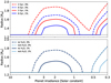 |
Fig. 4. Top (a): Planet radius vs. irradiance for sub-Neptunes with a mass of 2.5M⊕ and initial envelope mass fractions of 1% (solid lines) and 3% (dashed lines), at 2 and 6 Gyr. H2O/H2 is set to the saturation limit (dashed line in Fig. 3) up to a maximum of 0.1. Bottom (b): Same for sub-Neptunes at 4 Gyr with H2O as prescribed above, vs. those with envelopes without H2O. |
In water-poor systems, inefficient cooling will render primordial H/He envelopes around rocky cores more susceptible to hydrodynamic escape (Fig. 4b) as well as erosion by stellar winds. Infrared spectroscopy by Spizter and JWST has revealed that the chemistry of many inner protoplanetary disks around very low-mass stars (VLMS; ≲0.2 M⊙) is consistent with a high C/O ratio (Najita et al. 2013; Tabone et al. 2023; Arabhavi et al. 2024; Kanwar et al. 2024; Long et al. 2025). The sub-Neptunes arising from these disks might have high C/O, H2O-poor envelopes. Figure 4b shows that on orbits with super-terrestrial irradiance (< 0.06 au for an M2-type host) where planets are readily detected by transit surveys, these envelopes will completely escape by 4 Gyr. While temperate C/O-rich sub-Neptunes are predicted to contain abundant CH4 (Moses et al. 2013), this molecule is a less efficient radiator and is susceptible to UV photodissociation (Yoshida et al. 2024b,a). CO from disequilibrium mixing (Fortney et al. 2020) could be a source of O for the formation of H2 and OH, but its high molecular weight will limit its altitude distribution to the turbopause, where CO-dissociating far-UV photons are already absorbed by overlying CH4. Thus planets forming from high C/O disks will experience accelerated evaporation of their envelopes, which might explain the paucity of sub-Neptunes relative to rocky planets around VLMS compared to their FGK counterparts (Ment & Charbonneau 2023). Not all disks around VLMS are O-poor (Xie et al. 2023), and the exceptions might give rise to a surviving population of H2O-rich (or at least metal-rich) sub-Neptunes, for example, GJ 1214b (Ohno et al. 2025).
Similarly, protoplanetary disks around stars in binary systems with separations much less than ∼100 au are tidally truncated to a few au and are shorter lived (see Zagaria et al. 2023, and references therein). In these cases, the removal of icy O-rich (H2O and CO2) solids in the outer disk that would otherwise drift inward could lead to O- and H2O-poor planets in the inner disk. These H2O-poor objects would experience more rapid envelope escape, which might explain the deficit of detectable planets in these systems (Kraus et al. 2016), and in particular, the lack of sub-Neptunes relative to super-Earths (Sullivan et al. 2023).
The predicted decline in the abundance of H2O at irradiances below ∼3 times the solar constant (Fig. 3) can be detected by JWST using the method of transmission spectroscopy during transits (e.g. Benneke et al. 2024; Holmberg & Madhusudhan 2024). These observations probe the atmospheric composition at the 1–10 mbar level (Beichman & Greene 2018). All else being equal, indicators of atmospheric escape, for instance, anomalous absorption in H Lyman-α or the He triplet at 1083 nm, should be anticorrelated with the presence of H2O.
One caveat of our work is that we show outcomes for specific envelope mass fractions, whereas a population of sub-Neptunes would presumably have a distribution of values. Nevertheless, the overall trends with H2O/H2, irradiation, and stellar mass should hold. Another caveat is that the saturation concentration of H2O at the radiative-convective boundary should be considered an upper limit to the value in the upper atmosphere. The lower simulation boundary where H2O/H2 is fixed is at a number density of ∼1013 cm−3 and at an altitude above the turbopause, where the atmosphere ceases to be well mixed. Based on the eddy diffusivity relation for solar-metallicity atmospheres in Charnay et al. (2015) and a molecular diffusivity for H2 (Suárez-Iglesias et al. 2015), the turbopause is predicted to lie at a pressure altitude of 8.7 × 10⁻⁵ bar or a density of 2.3 × 1015 cm−3. This corresponds to several scale heights below the base of the thermosphere, and it might mean that H2O is significantly depleted by diffusion. H2O is also photodissociated by FUV radiation, but in a H-rich atmosphere the back reaction is efficient, and there should be an equilibrium between H2O and the principle photodissociation product O2 (e.g., Kawamura et al. 2024). An O2-rich layer will form on top of the H2O-rich atmosphere below and protect it from FUV radiation (inset of top panel of Fig. A.2). Finally, above a critical H2O/H2 (10−2 for solar metallicity and higher for supersolar), moist convection will be inhibited (Guillot 1995; Leconte et al. 2017), which will alter the pressure-temperature profile.
5. Conclusions
The hydrodynamic escape of H and He that is thought to cause the evolution of gas-rich sub-Neptunes into rock-dominated super-Earths is governed by the stellar EUV energy that is absorbed in the upper atmosphere relative to the energy of the escape from planetary gravity. This balance is modulated by IR and line emission by molecules and ions within the flow. We used a hydrodynamic escape model of a spherically symmetric, EUV-driven wind to demonstrate that the abundance of H2O in the upper atmosphere has a significant effect on escape rates. We list our results below.
-
An increase in the H2O abundance from 10−6 to 10−1 leads to a decrease in the escape rate by 1 dex, regardless of the surface gravity and XUV flux.
-
Sub-Neptunes just outside an irradiance level (approximately the solar constant) where saturation severely limits the H2O concentration in the upper atmosphere will experience a rapid decline in their radii relative to equivalent planets slightly closer to their host stars, potentially explaining the evolutionary trends inferred by Gaidos et al. (2024).
-
Sub-Neptunes that form around very low-mass stars (≲0.2 M⊙), which tend to have protoplanetary disks with H2O-poor chemistries consistent with a high C/O ratio, are likely to experience a more rapid escape, a possible explanation for their paucity around such stars.
-
A spectroscopic investigation of temperate sub-Neptune envelopes, for instance, by JWST, should reveal a marked decline in water content with lower irradiance, correlating with the paucity of such objects around older stars.
X-rays and far-UV radiation make only minor contributions to heating (e.g., Owen et al. 2020).
When H2O/H2 exceeds 0.1 the metallicity is > 100, the molecular weight is more than doubled, and together with increased cooling, planets are therefore less likely to have extended sub-Neptune-like atmospheres (Linssen et al. 2024).
Acknowledgments
TY was supported by JSPS KAKENHI Grant Nos. 23KJ0093 and 23H04645. EG was supported by NASA Awards 80NSSC20K0957 (Exoplanets Research Program) and 80NSSC21K0597 (Interdisciplinary Consortia for Astrobiology Research) and as a Gauss Professor at the University of Göttingen by the Niedersächsische Akaemie der Wissenschaften.
References
- Arabhavi, A. M., Kamp, I., Henning, T., et al. 2024, Science, 384, 1086 [NASA ADS] [CrossRef] [Google Scholar]
- Banks, P. M., & Kockarts, G. 1973, Aeronomy (Elsevier) [Google Scholar]
- Beichman, C. A., & Greene, T. P. 2018, in Handbook of Exoplanets, eds. H. J. Deeg, & J. A. Belmonte, 85 [Google Scholar]
- Benneke, B., Roy, P.-A., Coulombe, L.-P., et al. 2024, arXiv e-prints [arXiv:2403.03325] [Google Scholar]
- Berger, T. A., Huber, D., van Saders, J. L., et al. 2020, AJ, 159, 280 [Google Scholar]
- Bohren, C. F., & Albrecht, B. A. 1998, Atmospheric Thermodynamics (New York; Oxford: Oxford University Press) [Google Scholar]
- Catling, D. C., & Kasting, J. F. 2017, Atmospheric Evolution on Inhabited and Lifeless Worlds (Cambridge University Press) [CrossRef] [Google Scholar]
- Charnay, B., Meadows, V., & Leconte, J. 2015, ApJ, 813, 15 [Google Scholar]
- Cloutier, R., & Menou, K. 2020, AJ, 159, 211 [NASA ADS] [CrossRef] [Google Scholar]
- Dressing, C. D., & Charbonneau, D. 2015, ApJ, 807, 45 [Google Scholar]
- Fortney, J. J., Visscher, C., Marley, M. S., et al. 2020, AJ, 160, 288 [NASA ADS] [CrossRef] [Google Scholar]
- Fulton, B. J., Petigura, E. A., Howard, A. W., et al. 2017, AJ, 154, 109 [Google Scholar]
- Gaidos, E. J. 2000, Icarus, 145, 637 [Google Scholar]
- Gaidos, E., Hirano, T., Beichman, C., et al. 2022, MNRAS, 509, 2969 [Google Scholar]
- Gaidos, E., Claytor, Z., Dungee, R., Ali, A., & Feiden, G. A. 2023, MNRAS, 520, 5283 [Google Scholar]
- Gaidos, E., Ali, A., Kraus, A. L., & Rowe, J. F. 2024, MNRAS, 534, 3277 [Google Scholar]
- Guillot, T. 1995, Science, 269, 1697 [CrossRef] [Google Scholar]
- Hirano, T., Dai, F., Gandolfi, D., et al. 2018, AJ, 155, 127 [Google Scholar]
- Hirano, T., Livingston, J. H., Fukui, A., et al. 2021, AJ, 162, 161 [NASA ADS] [CrossRef] [Google Scholar]
- Holmberg, M., & Madhusudhan, N. 2024, A&A, 683, L2 [NASA ADS] [CrossRef] [EDP Sciences] [Google Scholar]
- Howard, A. W., Marcy, G. W., Bryson, S. T., et al. 2012, ApJS, 201, 15 [Google Scholar]
- Huebner, W., & Mukherjee, J. 2015, Planet. Space Sci., 106, 11 [Google Scholar]
- Hunten, D. M. 1973, J. Atmosp. Sci., 30, 1481 [Google Scholar]
- Johnstone, C. P., Güdel, M., Lammer, H., & Kislyakova, K. G. 2018, A&A, 617, A107 [NASA ADS] [CrossRef] [EDP Sciences] [Google Scholar]
- Johnstone, C. P., Bartel, M., & Güdel, M. 2021, A&A, 649, A96 [EDP Sciences] [Google Scholar]
- Kanwar, J., Kamp, I., Jang, H., et al. 2024, A&A, 689, A231 [NASA ADS] [CrossRef] [EDP Sciences] [Google Scholar]
- Kasting, J. F. 1988, Icarus, 74, 472 [NASA ADS] [CrossRef] [Google Scholar]
- Kawamura, Y., Yoshida, T., Terada, N., et al. 2024, ApJ, 967, 95 [Google Scholar]
- Kockarts, G. 1980, Geophys. Res. Lett., 7, 137 [NASA ADS] [CrossRef] [Google Scholar]
- Kraus, A. L., Ireland, M. J., Huber, D., Mann, A. W., & Dupuy, T. J. 2016, AJ, 152, 8 [NASA ADS] [CrossRef] [Google Scholar]
- Kubyshkina, D., Fossati, L., Erkaev, N. V., et al. 2018, A&A, 619, A151 [NASA ADS] [CrossRef] [EDP Sciences] [Google Scholar]
- Kuramoto, K., Umemoto, T., & Ishiwatari, M. 2013, Earth Planet. Sci. Lett., 375, 312 [CrossRef] [Google Scholar]
- Leconte, J., Selsis, F., Hersant, F., & Guillot, T. 2017, A&A, 598, A98 [NASA ADS] [CrossRef] [EDP Sciences] [Google Scholar]
- Le Teuff, Y., Millar, T., & Markwick, A. 2000, A&AS, 146, 157 [NASA ADS] [CrossRef] [EDP Sciences] [Google Scholar]
- Linssen, D., Shih, J., MacLeod, M., & Oklopčić, A. 2024, A&A, 688, A43 [NASA ADS] [CrossRef] [EDP Sciences] [Google Scholar]
- Long, F., Pascucci, I., Houge, A., et al. 2025, ApJ, 978, L30 [Google Scholar]
- Lopez, E. D., & Fortney, J. J. 2014, ApJ, 792, 1 [Google Scholar]
- Loyd, R. P., France, K., Youngblood, A., et al. 2016, ApJ, 824, 102 [NASA ADS] [CrossRef] [Google Scholar]
- Masson, A., Vinatier, S., Bézard, B., et al. 2024, A&A, 688, A179 [NASA ADS] [CrossRef] [EDP Sciences] [Google Scholar]
- McElroy, D., Walsh, C., Markwick, A., et al. 2013, A&A, 550, A36 [NASA ADS] [CrossRef] [EDP Sciences] [Google Scholar]
- Ment, K., & Charbonneau, D. 2023, AJ, 165, 265 [NASA ADS] [CrossRef] [Google Scholar]
- Mlynczak, M. G., Hunt, L. A., Garcia, R. R., et al. 2022, J. Geophys. Res. (Atmosp.), 127, e2022JD036767 [Google Scholar]
- Moses, J. I., Line, M. R., Visscher, C., et al. 2013, ApJ, 777, 34 [Google Scholar]
- Muñoz, A. G. 2007, Planet. Space Sci., 55, 1426 [Google Scholar]
- Murray-Clay, R. A., Chiang, E. I., & Murray, N. 2009, ApJ, 693, 23 [Google Scholar]
- Najita, J. R., Carr, J. S., Pontoppidan, K. M., et al. 2013, ApJ, 766, 134 [Google Scholar]
- Ohno, K., Schlawin, E., Bell, T. J., et al. 2025, ApJ, 979, L7 [Google Scholar]
- Orell-Miquel, J., Lampón, M., López-Puertas, M., et al. 2023, A&A, 677, A56 [NASA ADS] [CrossRef] [EDP Sciences] [Google Scholar]
- Owen, J. E. 2019, Ann. Rev. Earth Planet. Sci., 47, 67 [Google Scholar]
- Owen, J. E., & Wu, Y. 2013, ApJ, 775, 105 [Google Scholar]
- Owen, J., Shaikhislamov, I., Lammer, H., Fossati, L., & Khodachenko, M. 2020, Space Sci. Rev., 216, 1 [CrossRef] [Google Scholar]
- Petigura, E. A., Howard, A. W., & Marcy, G. W. 2013, Proc. Nat. Acad. Sci., 110, 19273 [Google Scholar]
- Petigura, E. A., Rogers, J. G., Isaacson, H., et al. 2022, AJ, 163, 179 [NASA ADS] [CrossRef] [Google Scholar]
- Piaulet-Ghorayeb, C., Benneke, B., Radica, M., et al. 2024, ApJ, 974, L10 [NASA ADS] [CrossRef] [Google Scholar]
- Pierrehumbert, R. T. 2023, ApJ, 944, 20 [NASA ADS] [CrossRef] [Google Scholar]
- Raymond, S. N., Scalo, J., & Meadows, V. S. 2007, ApJ, 669, 606 [Google Scholar]
- Robinson, T. D., & Catling, D. C. 2012, ApJ, 757, 104 [Google Scholar]
- Roble, R. G., & Dickinson, R. E. 1989, Geophys. Res. Lett., 16, 1441 [Google Scholar]
- Rockcliffe, K. E., Newton, E. R., Youngblood, A., et al. 2023, AJ, 166, 77 [NASA ADS] [CrossRef] [Google Scholar]
- Rothman, L. S., Gordon, I. E., Babikov, Y., et al. 2013, J. Quant. Spectr. Rad. Transf., 130, 4 [Google Scholar]
- Salz, M., Schneider, P., Czesla, S., & Schmitt, J. 2016, A&A, 585, L2 [NASA ADS] [CrossRef] [EDP Sciences] [Google Scholar]
- Suárez-Iglesias, O., Medina, I., Sanz, M. D. L. A., Pizarro, C., & Bueno, J. L., 2015, J. Chem. Eng. Data, 60, 2757 [Google Scholar]
- Sullivan, K., Kraus, A. L., Huber, D., et al. 2023, AJ, 165, 177 [NASA ADS] [Google Scholar]
- Tabone, B., Bettoni, G., van Dishoeck, E. F., et al. 2023, Nat. Astron., 7, 805 [NASA ADS] [CrossRef] [Google Scholar]
- Tennyson, J., Yurchenko, S. N., Al-Refaie, A. F., et al. 2016, J. Mol. Spectrosc., 327, 73 [Google Scholar]
- Tian, F., Toon, O. B., Pavlov, A. A., & De Sterck, H. 2005, ApJ, 621, 1049 [Google Scholar]
- Turbet, M., Bolmont, E., Ehrenreich, D., et al. 2020, A&A, 638, A41 [NASA ADS] [CrossRef] [EDP Sciences] [Google Scholar]
- Van Eylen, V., Astudillo-Defru, N., Bonfils, X., et al. 2021, MNRAS, 507, 2154 [NASA ADS] [Google Scholar]
- Venturini, J., Ronco, M. P., Guilera, O. M., et al. 2024, A&A, 686, L9 [NASA ADS] [CrossRef] [EDP Sciences] [Google Scholar]
- Weiss, L. M., & Marcy, G. W. 2014, ApJ, 783, L6 [Google Scholar]
- Xie, C., Pascucci, I., Long, F., et al. 2023, ApJ, 959, L25 [NASA ADS] [CrossRef] [Google Scholar]
- Yabe, T., & Aoki, T. 1991, Comput. Phys. Commun., 66, 219 [Google Scholar]
- Yoshida, T., & Kuramoto, K. 2020, Icarus, 345, 113740 [NASA ADS] [CrossRef] [Google Scholar]
- Yoshida, T., & Kuramoto, K. 2021, MNRAS, 505, 2941 [NASA ADS] [CrossRef] [Google Scholar]
- Yoshida, T., Terada, N., Ikoma, M., & Kuramoto, K. 2022, ApJ, 934, 137 [NASA ADS] [CrossRef] [Google Scholar]
- Yoshida, T., Koyama, S., Nakamura, Y., Terada, N., & Kuramoto, K. 2024a, Astrobiology, 24, 1074 [Google Scholar]
- Yoshida, T., Terada, N., & Kuramoto, K. 2024b, Prog. Earth Planet. Sci., 11, 59 [Google Scholar]
- Zagaria, F., Rosotti, G. P., Alexander, R. D., & Clarke, C. J. 2023, Eur. Phys. J. Plus, 138, 25 [NASA ADS] [CrossRef] [Google Scholar]
- Zhang, M., Knutson, H. A., Dai, F., et al. 2023, AJ, 165, 62 [NASA ADS] [CrossRef] [Google Scholar]
Appendix A: Atmospheric Profiles
Fig. A.1 shows the dependence of the outflow temperature profile on basal H2O/H2 subjected to stellar EUV 103× the present terrestrial value, with Mp = 5M⊕ and g = 4 m s−2. Fig. A.2 shows profiles of the number density, heating, and cooling rate in a flow with the same parameters, except only for a basal H2O/H2 ratio of 10−3, In the lower region of the flow (r ≲ 2Rp), the temperature decreases with increasing basal H2O/H2 ratio up to ∼0.01 as a result of greater radiative cooling. As shown in Fig. A.2, H2O is the primary coolant in this lower region. Along the outflow, H2O is photolyzed to H, O, OH, and various ions. As a result, cooling by photochemical products, especially H and OH+, is significant at higher altitudes. As the basal H2O/H2 ratio approaches ∼0.1, the mean molecular weight of the flow increases, reducing the speed of the outflow and the contribution of adiabatic cooling, and temperatures in the lower region of the flow begin to increase. This dependence on the mean molecular weight is discussed in detail by Yoshida & Kuramoto (2020).
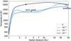 |
Fig. A.1. Temperature profile (radial coordinate in units of planet radius) in a hydrodynamic flow for different lower boundary values H2O/H2 with a stellar EUV flux of |


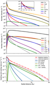 |
Fig. A.2. Top: Number density profiles of neutral species with a basal H2O/H2 of 0.001, stellar EUV flux of |

Appendix B: Mass fractionation between H and O
Fig. B1 shows the fractionation factor between H and O, defined as (FO/FH)/(nO(r0)/nH(r0)), where Fi and ni(r0) are the escape rate and the total number density at the lower boundary r0 of element i, respectively. This ratio decreases (fractionation increases) as the H2O/H2 ratio increases or as the EUV flux decreases, due to the reduced H escape flux and less efficient O drag.
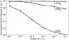 |
Fig. B.1. Fractionation factor between H and O for different values of interior H2O/H2 and stellar EUV flux with a surface gravity of 4 m s−2 and planet mass of 5M⊕. |
Appendix C: Escape timescale as a function of initial atmospheric mass and stellar flux
Fig. C1 shows the escape timescale of pure H2 atmosphere as a function of stellar flux and initial atmospheric mass with a planetary mass of 2.5Mp, where the timescale is defined as the duration required for the atmospheric mass to reach 10−4Mp. The timescale exhibits weak dependence on the initial atmospheric mass because the escape rate increases with initial atmospheric mass due to planetary inflation and the resulting decrease in gravitational acceleration at the base of the outflow.
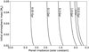 |
Fig. C.1. Escape timescale of pure H2 atmospheres as a function of stellar irradiance and initial envelope mass with a planet mass of 2.5M⊕. |
Appendix D: Model details
D.1. Basic equations
We solve the fluid equations of continuity, momentum and energy for a multi-component gas, assuming a spherically symmetric flow:
 (D.1)
(D.1)
 (D.2)
(D.2)
![Mathematical equation: $$ \begin{aligned} \frac{\partial }{\partial t}\left[\rho \left(\frac{1}{2}u^{2}+E\right)\right]+\frac{1}{r^{2}}\frac{\partial }{\partial r}\left\{ \left[\left(\frac{1}{2}u^{2}+E+\frac{p}{\rho }\right)\rho u \right]r^{2}\right\} =-\frac{GM_{p}}{r^{2}}\rho u+q, \end{aligned} $$](/articles/aa/full_html/2025/04/aa53667-25/aa53667-25-eq15.gif) (D.3)
(D.3)
where t is the time, r is the distance from the planet’s center, ni, ρi, ui, pi, and ωi are the number density, mass density, velocity, partial pressure, and production rate of species i, respectively, G is the gravitational constant, Mp is the mass of the planet, ρ, p, and E are the total mass density, total pressure, and total specific internal energy, respectively, u is the mean gas velocity, μij is the reduced molecular mass between species i and j, kij is the momentum transfer collision frequency that follows
 (D.4)
(D.4)
where kB is the Boltzmann constant and T is the temperature. bij is the binary diffusion coefficient given by
 (D.5)
(D.5)
where α is the polarizability (Banks & Kockarts 1973; Muñoz 2007). Here, bij, T, μij and α are expressed in cm−1s−1, K, g and cm3, respectively. The total internal energy is given by
 (D.6)
(D.6)
where n is the total number density and γi is the ratio of specific heat of species i. The net heating rate is given by
 (D.7)
(D.7)
where qabs is the heating rate by X-ray and UV absorption (see D.3), qch is the rate of net chemical expense of energy (see D.2), and qrad is the radiative cooling rate by IR active molecules (see D.3).
D.2. Chemistry
A total of 93 chemical reactions are considered for 15 atmospheric components: H2, H2O, H, O, O(1D), OH, O2, H+, H , H
, H , O+, O
 , OH+, H2O+, and H3O+ (Table A1 and A2).
The photolysis rate fph, i is given by
 (D.8)
(D.8)
where σi(λ) is the photodissociation/photoionization cross section at wavelength λ for species i and I(λ) is the incident X-ray/UV photon flux at wavelength λ. The energy consumed per unit time by this photolysis qph, i is given by
 (D.9)
(D.9)
where λth, i is the threshold wavelength for the photolysis of species i, h is the Planck constant, and c is the speed of light in vacuum. We adopt the photodissociation and photoionization cross sections provided by “PHoto Ionization/Dissociation RATES”3 (Huebner & Mukherjee 2015).
In addition to photolysis reactions, this study considers bimolecular reactions. The bimolecular reaction rate fR can be written as
 (D.10)
where ni and nj represent the number densities of reactant i and j, respectively, and kR is the corresponding reaction rate coefficient. We use the reaction rate coefficients provided by The UMIST Database for Astrochemistry 20124 (McElroy et al. 2013). We neglect the formation of molecules that have more than one carbon atom because of the low densities in the outflow. The energy consumed per unit time by a bimolecular reaction is given by
 (D.11)
where ΔER is the heat of reaction, which is positive for endothermic reactions and negative for exothermic reactions. In evaluating the heats of reaction, we make use of the enthalpies of formation listed in Le Teuff et al. (2000). The energy consumption rate qch is calculated by summing the consumed amounts of energy by individual chemical reactions including photolysis.
D.3. Radiative processes
In order to calculate the radial profiles of rates of heating and photolysis in the atmosphere, we model the radiative transfer of parallel stellar photon beams in a spherically symmetric atmosphere by applying the method formulated by Tian et al. (2005). We consider X-ray and UV absorption by H2, H2O, H, O, OH, and O2. The stellar beam is assumed to be absorbed by Beer’s law. The energy deposition in a given layer along each path is then multiplied by the area of the ring (Fig. 6 in Tian et al. 2005) to obtain the total energy deposited into the shell segment. The volumetric heating rate qabs is given by the total energy absorbed per unit time by each shell divided by the volume of the shell. We adopt the X-ray and UV spectrum from 0.1 to 280 nm estimated for GJ 832 as a representative M2 dwarf (Loyd et al. 2016). The EUV flux at 1 au is taken to be 1.1 × 10⁻³ Wm−2, which is about 0.25 times that from the present Sun. To represent both the higher EUV luminosity typical of young stars and a range of semi-major axes, we scale the stellar spectrum to consider EUV fluxes up to 104 times the Earth’s level.
We consider radiative cooling by thermal line emission of H2O, OH, H , OH+, and H3O+. The radiative cooling rate due to a transition from energy level i to j of radiatively active molecular species s is given by
 (D.12)
where ns, i is the population density in level i, Aij is the spontaneous transition probability, hνij is the energy difference between level i and level j, and βij is the photon escape probability. The total radiative cooling rate by species s is calculated by summing the radiative cooling rates of all the transitions. The population density ns, i is calculated under the assumption of local thermodynamic equilibrium as
 (D.13)
where ns and Z are the total number density and partition function of species s, and gi and Ei are the statistical weight and energy of level i. Approximating that half of the photons are emitted upward while the other half is emitted downward and then absorbed by dense, lower atmospheric layers, the bulk escape probability is evaluated by
![Mathematical equation: $$ \begin{aligned} \beta _{ij}(r)=\frac{1}{2}\int _{0}^{\infty }\phi (\nu ,r)\,\mathrm{exp} \left[-\int _{r_{\mathrm{top} }}^{r}\alpha _{\mathrm{L} _{ij}}\phi (\nu ,r)dr\right] d\nu \end{aligned} $$](/articles/aa/full_html/2025/04/aa53667-25/aa53667-25-eq30.gif) (D.14)
(D.14)
where rtop is the radius of the outer boundary (the top of the atmosphere), αLij is the absorption coefficient integrated over frequency, and ϕ(ν, r) is the line profile, αLij is given by
 (D.15)
Assuming a Doppler-broadened line profile, ϕ(ν, r) is given by
![Mathematical equation: $$ \begin{aligned} \phi (\nu ,r)=\frac{1}{\sqrt{\pi }\Delta \nu _{\rm D}}\mathrm{exp} \left[-\frac{1}{(\Delta \nu _{\rm D})^{2}}\left(\nu - \nu _{0}-\frac{u_{s}(r)}{c}\nu _{0}\right)^{2}\right], \end{aligned} $$](/articles/aa/full_html/2025/04/aa53667-25/aa53667-25-eq32.gif) (D.16)
(D.16)
where us(r) is the velocity profile of radiative sources and ν0 is the rest-frame central frequency of the line profile; and ΔνD is the Doppler width given by
 (D.17)
where ms is the molecular mass of species s. The net radiative cooling rate qrad is obtained by the sum of contributions by H2O, OH, H , and OH+. We use the line data provided by the HITRAN database5 (Rothman et al. 2013) and ExoMol database6(Tennyson et al. 2016). We consider 31,333 transitions of H2O and 4043 transitions of OH to cover over 99% of total energy emission within the 100–3000 K temperature range. The emission from H
 , OH+, and H3O+ are assumed to be optically thin throughout the flow, with all lines from the ExoMol database (Tennyson et al. 2016).
Chemical reactions included in the model
Chemical reactions (continued)
D.4. Calculation method
The governing equations are solved by numerical time integration until the physical quantities reach their steady-state profiles. These equations can be split into advection phases and non-advection phases. We employ the CIP method to solve for the advection phases (Yabe & Aoki 1991) to achieve numerical stability and accuracy for hydrodynamic escape simulations (Kuramoto et al. 2013). After solving the advection phases, we solve the non-advection phases with a finite-difference approach. The non-advection phases of the energy equation are solved explicitly. Those of the continuity equations are solved with the semi-implicit method. Those of the momentum equations are solved implicitly using the quantities for the next time step that are obtained by the integration of the energy equation and the continuity equations.
1000 spatial grids in radial coordinates are taken with the grid-to-grid intervals exponentially increasing with r. The time step is defined so as to satisfy the CFL condition. For each parameter setup, we continue the time integration until reaching the steady state using the convergence condition described in Tian et al. (2005).
The lower and upper boundaries are set to r = Rp, 50 Rp, respectively, where Rp is the radius of the planet. In each simulation run, the atmospheric density and temperature at the lower boundary are fixed. We assume that only H2 and H2O exist at the lower boundary. The number density of H2 at the lower boundary is set to 1 × 10¹⁹ m−3. The number density of H2O is given as a parameter in each simulation run. The temperature at the lower boundary is set to 400 K. This corresponds to the skin temperature, the asymptotic temperature at high altitudes of the upper atmosphere that is optically thin in the thermal-IR and transparent to shortwave radiation (Catling & Kasting 2017). The other physical quantities at the lower and upper boundaries are estimated by linear extrapolations from the calculated domain. As the initial condition, we use the steady-state profiles of the pure H2 atmosphere and add H2O whose number density profiles are given by the hydrostatic structure. The initial velocity of H2O is set at 1 × 10⁻⁵ m s−1.
Appendix E: Water abundance in the upper atmosphere
Even if the lower atmosphere contains plentiful H2O (as steam), the abundance in the upper atmosphere can be ultimately limited by the saturation vapor pressure where it is lowest relative to the total local pressure. Figure E1 plots a schematic radiative-convective (R-C) atmosphere where the upper radiative zone is uniformly at the skin temperature Teq/20.25 (here set to the Earth-like value of 255 K), and the convective zone is an adiabat with γ = 1.4, appropriate for H2. The R-C boundary (circle) is set at 0.1 bar, a value which is typical for Solar System atmospheres (Robinson & Catling 2012). Curves of the saturation vapor-pressure over ice or liquid H2O (Bohren & Albrecht 1998), scaled for different mixing ratios, are plotted. Water vapor in rising atmospheric parcels will condense out and form clouds up to a maximum altitude at the R-C boundary where the vapor pressure is lowest. The H2O/H2 ratio at that boundary and higher altitudes is then set by the saturation vapor pressure curve that intersects the R-C boundary point (in this case, 1.3 × 10⁻⁴). Lower or higher Teq results in lower or higher H2O/H2, accordingly, and this variation describes the curve in Fig. 3. (The curve is not sensitive to the exact location of the R-C boundary). that the turbopause, above which molecular diffusion dominates over eddy diffusion, is predicted to lie at ∼10−4 bar, well above the plot.
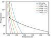 |
Fig. E.1. Pressure-temperature profile (black curve) in a simplified H2-rich atmosphere with a radiative-convective boundary at 0.1 bar pressure (black point). The colored lines represent the vapor pressures for different H2O/H2 mixing ratios, and the lowest vapor pressure along the profile occurs at the R-C boundary (black filled circle). |
All Tables
All Figures
|
Fig. 1. Total escape rate vs. H2O/H2 for different values of EUV irradiance at fixed surface gravity g = 4 m s−2 (top panel) and for different values of g at a fixed EUV irradiance of 103F⊕ (bottom panel). Mp is fixed at 5M⊕. The dashed lines are from Eqs. (1)–(3). |
| In the text | |
|
Fig. 2. Evolution of the EUV flux (top panel, a), escape rate (b), envelope mass (c), and planet radius (d) for a planet with Mp = 2.5M⊕, an initial envelope mass fraction of 1%, and different initial values of H2O/H2 on an orbit with a main-sequence stellar irradiance equal to the terrestrial value. The solid (dashed) lines represent results without (with) mass fractionation between H and O. The mass fractionation results are omitted from panel b for clarity. |
| In the text | |
|
Fig. 3. Lifetime of envelopes with initial mass fraction of 1% on Mp = 2.5M⊕ sub-Neptunes as a function of stellar irradiance and H2O/H2. The dashed line is the saturation-limited H2O/H2 ratio in the upper atmosphere (see text and Appendix C). The stars represent the scenarios in Fig. 2. |
| In the text | |
|
Fig. 4. Top (a): Planet radius vs. irradiance for sub-Neptunes with a mass of 2.5M⊕ and initial envelope mass fractions of 1% (solid lines) and 3% (dashed lines), at 2 and 6 Gyr. H2O/H2 is set to the saturation limit (dashed line in Fig. 3) up to a maximum of 0.1. Bottom (b): Same for sub-Neptunes at 4 Gyr with H2O as prescribed above, vs. those with envelopes without H2O. |
| In the text | |
|
Fig. A.1. Temperature profile (radial coordinate in units of planet radius) in a hydrodynamic flow for different lower boundary values H2O/H2 with a stellar EUV flux of |
| In the text | |
|
Fig. A.2. Top: Number density profiles of neutral species with a basal H2O/H2 of 0.001, stellar EUV flux of |
| In the text | |
|
Fig. B.1. Fractionation factor between H and O for different values of interior H2O/H2 and stellar EUV flux with a surface gravity of 4 m s−2 and planet mass of 5M⊕. |
| In the text | |
|
Fig. C.1. Escape timescale of pure H2 atmospheres as a function of stellar irradiance and initial envelope mass with a planet mass of 2.5M⊕. |
| In the text | |
|
Fig. E.1. Pressure-temperature profile (black curve) in a simplified H2-rich atmosphere with a radiative-convective boundary at 0.1 bar pressure (black point). The colored lines represent the vapor pressures for different H2O/H2 mixing ratios, and the lowest vapor pressure along the profile occurs at the R-C boundary (black filled circle). |
| In the text | |
Current usage metrics show cumulative count of Article Views (full-text article views including HTML views, PDF and ePub downloads, according to the available data) and Abstracts Views on Vision4Press platform.
Data correspond to usage on the plateform after 2015. The current usage metrics is available 48-96 hours after online publication and is updated daily on week days.
Initial download of the metrics may take a while.