© The Authors 2025

1. Introduction

Understanding the mechanism driving angular momentum transport in turbulent magnetized disks is key to moving beyond models based on enhanced viscosity, as originally introduced by Shakura & Sunyaev (1973) and Lynden-Bell & Pringle (1974). The inherent differential rotation present in astrophysical disks has the potential to produce unstable magnetic fields with a wide range of properties (Velikhov 1959; Chandrasekhar 1960; Balbus & Hawley 1991, 1992; Pessah & Psaltis 2005; Johansen & Levin 2008; Pessah & Chan 2012; Das et al. 2018; Mamatsashvili et al. 2020; Squire et al. 2024; Brughmans et al. 2024). Ionized rotating fluids with angular frequency profiles decreasing outwards are particularly prone to developing the so-called magnetorotational instability (MRI) when threaded by a weak magnetic field in the direction perpendicular to the shear (Balbus & Hawley 1991). The turbulence driven by the MRI is considered a leading mechanism enabling accretion in astrophysical disks around compact objects (Balbus & Hawley 1998).

The conditions for the onset of the MRI can be fulfilled in other important astrophysical scenarios. For example, protoneutron stars (PNSs) that result from the core collapse of rotating massive stars can possess regions where the MRI grows faster than the explosion timescale (Akiyama et al. 2003; Obergaulinger et al. 2006; Cerdá-Durán et al. 2008; Rembiasz et al. 2016a; Reboul-Salze et al. 2021). The MRI can also develop in the binary neutron star (BNS) postmerger phase (Duez et al. 2006a,b; Siegel et al. 2013; Kiuchi et al. 2018, 2024; Fernández et al. 2019; Held & Mamatsashvili 2022; Held et al. 2024). Depending on the total mass of the binary, the system may go through the formation of a short-lived postmerger object, a so-called hypermassive neutron star. This object eventually collapses to a black hole once the support against gravity by rotation or neutrino pressure lessens. During this phase, the MRI can lead to efficient angular momentum transport and magnetic field amplification that could have important consequences on the dynamics of the postmerger remnant. The efficiency of the angular momentum transport is directly related to the timescale in which the black hole forms. Moreover, magnetic field amplification can generate large-scale structures that seem to favor jet formation and short gamma-ray bursts (Rezzolla et al. 2011; Ruiz et al. 2016; Combi & Siegel 2023; Bamber et al. 2024). Another scenario where the MRI plays a role involves neutron star – black hole mergers (Etienne et al. 2012; Paschalidis et al. 2015; Kiuchi et al. 2015; Ruiz et al. 2018; Christie et al. 2019). The instability sets in when an accretion disk is formed around the black hole after the merger.

Due to the relevance of the MRI in many astrophysical settings, significant effort has been devoted to unraveling the physics of the instability and the resulting turbulent state. Seed perturbations can grow exponentially on timescales close to the rotational period. These perturbations take the form of so-called channel modes, which are pairs of vertically stacked layers in which the velocity and the magnetic field perturbations have radial and azimuthal components of (sinusoidally) alternating polarity. These modes have associated Maxwell and Reynolds stresses that lead to outward transport of angular momentum (Goodman & Xu 1994; Pessah et al. 2006a; Pessah & Chan 2008).

The growth of the instability eventually terminates, resulting in the breakdown of the channels into small-scale turbulence. The details of the processes involved in the saturation of the MRI, including the factor by which the seed perturbations are amplified, are not yet completely understood. Several authors (Hawley et al. 1995; Brandenburg et al. 1995; Fleming et al. 2000; Sano & Inutsuka 2001; Sano et al. 2004; Gardiner & Stone 2005; Pessah et al. 2007; Vishniac 2009; Davis et al. 2010; Murphy & Pessah 2015; Rembiasz et al. 2016a,b; Hirai et al. 2018; Gogichaishvili et al. 2018) have provided further insight into the saturation of the MRI and the resulting nonlinear turbulent regime by performing numerical box simulations and also (semi-)global simulations of accretion disks (Sorathia et al. 2010, 2012; Hawley et al. 2011), fast rotating PNSs (Obergaulinger et al. 2009; Mösta et al. 2015; Reboul-Salze et al. 2022) and BNS merger remnants (Kiuchi et al. 2018; Shibata et al. 2021).

Goodman & Xu (1994) presented a model for parasitic instabilities (PIs) that was further developed with local linear analyses by Lesaffre et al. (2009), Latter et al. (2009), Pessah & Goodman (2009), and Pessah (2010), among others. This model provides a physical mechanism that explains the termination of the MRI and the onset of the nonlinear regime. Laminar channel flows can be unstable against PIs that can be of Kelvin-Helmholtz (KH) or tearing-mode (TM) type, depending on the value of kinematic viscosity and resistivity, that is, nonideal effects. At the beginning of the exponential growth of the MRI, the effect of the PIs is negligible, since they grow much slower than the MRI. Nevertheless, the growth rate of the PIs is proportional to the amplitude of the MRI modes, which grows exponentially in time. This means that, at some point, the PIs start growing much faster than the MRI modes, and they eventually disrupt the channel modes and saturate the MRI, leading to a turbulent regime. The predictions made by these analytical approaches have been tested by several numerical magnetohydrodynamic (MHD) simulations (Latter et al. 2009, 2010; Longaretti & Lesur 2010; Lesur & Longaretti 2011; Murphy & Pessah 2015; Rembiasz et al. 2016a,b; Hirai et al. 2018), but there are still some discrepancies between the analytical models and the numerical results.

Pessah & Goodman (2009) and Pessah (2010) performed an analytical study in resistive-viscous MHD of the evolution of PIs by solving an eigenvalue problem with linear equations for these secondary instabilities. They exhaustively covered a huge parameter space to identify the fastest growing parasitic modes for different values of kinematic viscosity and resistivity. The authors (and also Latter et al. 2009) made several assumptions to make the problem more tractable. The most notable simplifications are the consideration of the primary MRI mode as a time-independent background, and the assumption that the wavevectors of the parasitic modes are also time-independent (see Sect. 3.1 in Pessah 2010 for a critical assessment of the assumptions involved).

In this work, we relax some simplifications made in previous studies to obtain a more accurate description of the evolution of PIs and a better estimate of the saturation of the MRI. Building on the approach in Pessah (2010), we derive a set of equations for the parasitic perturbations feeding of the fastest growing MRI mode for a fixed vertical magnetic field. However, here we account for the exponential growth of the MRI modes and the linear shear of the parasitic wavevector induced by differential rotation of the background flow¹. By covering a dense parameter space, we identify the fastest secondary modes that lead to the saturation of the MRI. Using different values for the seed perturbations, we obtain amplification factors of the MRI that are similar to the ones obtained in the numerical simulations presented in Rembiasz et al. (2016b).

The paper is organized as follows: in Sect. 2, we state our working assumptions and present the equations for the PIs. In Sect. 3, we present the results of a systematic exploration to find the fastest parasitic modes responsible for the saturation of the MRI. We showcase the time evolution of several parasitic modes to provide physical intuition on the elements playing a role in the saturation process. In Sect. 4, we present our effective model for field amplification driven by the MRI and provide a expression for the MRI magnetic field at saturation. In Sect. 5, we compare our findings with numerical simulations. We discuss the implications of our findings in Sect. 6.

2. Parasitic instabilities feeding off exponential MRI modes

To carry out a linear analysis of the parasitic modes feeding off the MRI channels, we need to treat those channels as part of the background fields, as in Goodman & Xu (1994), Pessah & Goodman (2009) and Pessah (2010). This is a sensible approach during the MRI growth, since the amplitude of the channel modes is much larger than the parasitic ones. This implies that the primary instability (the MRI) is not significantly affected by the secondary (parasitic modes) until they reach a similar amplitude. This approximation is bound to break down when the amplitudes involved are comparable. Nevertheless, here we consider that the primary MRI mode grows exponentially unimpeded. The novelty compared to previous studies is that we do consider that the parasites, with shearing time-dependent wavevectors, are feeding from a time-dependent MRI mode.

We consider the system of incompressible MHD equations governing the dynamics of the velocity V and magnetic B fields in the shearing box approximation (Hawley et al. 1995)

$$\begin{array}{cc}\hfill {\partial }_t\mathit{V}+(\mathit{V}·\mathrm{\nabla })\mathit{V}& =-2\mathbf{\Omega }\times \mathit{V}+q{\mathrm{\Omega }}^2\mathrm{\nabla }(x^2)-\frac{1}{\rho }\mathrm{\nabla }(P+\frac{B^2}{8\pi })\hfill \end{array}$$(1)

$$\begin{array}{cc}& +\frac{(\mathit{B}·\mathrm{\nabla })\mathit{B}}{4\pi \rho }+\nu {\mathrm{\nabla }}^2\mathit{V},\hfill \\ \hfill {\partial }_t\mathit{B}+(\mathit{V}·\mathrm{\nabla })\mathit{B}& =(\mathit{B}·\mathrm{\nabla })\mathit{V}+\eta {\mathrm{\nabla }}^2\mathit{B},\hfill \end{array}$$(2)

$$\begin{array}{cc}\hfill \mathrm{\nabla }·\mathit{V}& =0,\hfill \end{array}$$(3)

$$\begin{array}{cc}\hfill \mathrm{\nabla }·\mathit{B}& =0.\hfill \end{array}$$(4)

Here, $\mathbf{\Omega }=\mathrm{\Omega }\check{\mathbf{z}}$ stands for the angular frequency and q is the shear parameter

$$\begin{array}{c}\hfill q\equiv -\frac{dln\mathrm{\Omega }}{dlnr}{|}_{r_0},\end{array}$$(5)

both of these quantities are evaluated at some fiducial radius r₀. P stands for pressure, ρ is the density, whereas ν and η are the viscosity and resistivity. In what follows we simply write Ω for the local value of the angular frequency.

2.1. Equations of motion for the parasitic modes

The equations of motion for the PIs are obtained by seeking solutions for the total velocity and magnetic fields of the form (Goodman & Xu 1994):

$$\begin{array}{c}\hfill \left[\begin{array}{c}{V}_x\\ V_y\\ V_z\\ B_x\\ B_y\\ B_z\end{array}\right]=\left[\begin{array}{c}0\\ -q\mathrm{\Omega }x\\ 0\\ 0\\ 0\\ {\overline{B}}_z\end{array}\right]+\left[\begin{array}{c}{V}_x^{\mathrm{MRI}}\\ V_y^{\mathrm{MRI}}\\ 0\\ B_x^{\mathrm{MRI}}\\ B_y^{\mathrm{MRI}}\\ 0\end{array}\right]+\left[\begin{array}{c}{v}_x\\ v_y\\ v_z\\ b_x\\ b_y\\ b_z\end{array}\right].\end{array}$$(6)

Here, we include, from left to right, the contribution of the background shear flow ${\mathit{V}}_{\mathrm{sh}}=-q\mathrm{\Omega }x\check{\mathbf{y}}$, the vertical magnetic field ${\overline{B}}_z$, the MRI fields (that also constitute the background dynamics of our problem), and the parasitic fields. For absent secondary perturbations, the vertical magnetic field ${\overline{B}}_z$ remains unchanged and the MRI grows exponentially unaffected. The former assumption holds in the incompressible limit because the MRI itself does not feed back into ${\overline{B}}_z$ (Pessah et al. 2006a). This is a reasonable assumption in the context of local, shearing box simulations with an imposed vertical magnetic field, since the magnetic flux over the vertical boundaries is conserved when the usual azimuthally periodic boundary conditions are adopted. The second assumption is bound to break down when the parasitic mode amplitude is comparable to the amplitude of the MRI mode from which they feed. We address this issue in Sect. 5.

In the ideal, that is, for sufficiently small values of the viscosity ν and the resistivity η, incompressible MHD regime, the MRI evolves as an exact, nonlinear solution with a mode structure given by (Goodman & Xu 1994; Pessah et al. 2006a; Pessah & Chan 2008)

$$\begin{array}{cc}\hfill {\mathit{V}}^{\mathrm{MRI}}& =V_0(t)sin(K_{\mathrm{MRI}}z)[cos({\theta }_V)\check{\mathbf{x}}+sin({\theta }_V)\check{\mathbf{y}}],\hfill \end{array}$$(7)

$$\begin{array}{cc}\hfill {\mathit{B}}^{\mathrm{MRI}}& =B_0(t)cos(K_{\mathrm{MRI}}z)[cos({\theta }_B)\check{\mathbf{x}}+sin({\theta }_B)\check{\mathbf{y}}],\hfill \end{array}$$(8)

where V₀(t) = V₀e^γ_MRIt and B₀(t) = B₀e^γ_MRIt are the time-dependent MRI velocity and magnetic field amplitudes, respectively, $\check{\mathbf{x}}$ is the unit vector in the radial direction, $\check{\mathbf{y}}$ is the unit vector in the azimuthal direction, and θ_V and θ_B are the directions of the channels with respect to the radial direction. The fastest growing rate

$$\begin{array}{c}\hfill {\gamma }_{\mathrm{MRI}}=\frac{q}{2}\mathrm{\Omega },\end{array}$$(9)

is attained for the MRI mode with vertical wavenumber

$$\begin{array}{c}\hfill K_{\mathrm{MRI}}=\sqrt{1-\frac{{(\kappa /\mathrm{\Omega })}^4}{16}}\frac{\mathrm{\Omega }}{{\overline{v}}_{\mathrm{A}z}^2},\end{array}$$(10)

where $\kappa \equiv \sqrt{2(2-q)}\mathrm{\Omega }$ is the epicyclic frequency, and ${\overline{v}}_{\mathrm{A}z}$ corresponds to the Alfvén velocity. The physical structure of the fastest MRI mode is such that θ_V = π/4 and θ_B = 3π/4. The ratio between the MRI amplitudes in the ideal MHD limit, as found by Pessah & Chan (2008), is

$$\begin{array}{c}\hfill \frac{V_0}{B_0/\sqrt{4\pi \rho }}=\sqrt{\frac{4-{(\kappa /\mathrm{\Omega })}^2}{4+{(\kappa /\mathrm{\Omega })}^2}}·\end{array}$$(11)

As in Pessah (2010), we employ dimensionless variables defined in terms of the characteristic scales of length and time set by the background magnetic field and the local angular frequency: $L_0\equiv {\overline{v}}_{\mathrm{A}z}^2/\mathrm{\Omega }={\overline{B}}_z^2/(4\pi \rho \mathrm{\Omega })$ and T₀ ≡ 1/Ω. With this, ${\overline{B}}_z$ sets the scale for all magnetic and velocity fields. From now on, we omit the subscript “MRI” and use K, V and B to refer to the wavenumber, velocity, and magnetic fields associated with the fastest MRI mode. We absorb the factor $\sqrt{4\pi \rho }$ in the magnetic field, effectively working with Alfvén velocities.

The secondary, parasitic velocity and magnetic fields can be expressed as

$$\begin{array}{cc}\hfill \mathit{v}& =e^{i{\mathit{k}}_{\mathbf{h}}·\mathit{x}}\mathit{u}(t,z),\hfill \end{array}$$(12)

$$\begin{array}{cc}\hfill \mathit{b}& =e^{i{\mathit{k}}_{\mathbf{h}}·\mathit{x}}\mathit{w}(t,z),\hfill \end{array}$$(13)

where the explicit temporal dependence of the horizontal wavevector is given by

$$\begin{array}{c}\hfill {\mathit{k}}_{\mathbf{h}}=(k_x(0)+q\mathrm{\Omega }{k}_{y}t)\check{\mathbf{x}}+k_y\check{\mathbf{y}}.\end{array}$$(14)

This simply reflects the fact that wave crests are swept by the (linear) shear background flow, thereby increasing their wavenumber and rotating toward the radial direction, $\check{\mathbf{x}}$ (Latter et al. 2010; Mamatsashvili et al. 2013).

We can exploit the incompressible nature of the flow and focus on the dynamics in the plane (${\stackrel{\mathbf{ˇ}}{\mathit{k}}}_{\mathbf{h}},\check{\mathbf{z}}$) (Pessah 2010). In fact, this condition restricts our problem to one single direction, since ik_h ⋅ v_h = −∂_zv_z. We can furthermore eliminate the pressure by using the divergenceless condition for the velocity [Eq. (3)]. Then, the evolution equations for the vertical components of the parasitic velocity and magnetic fields become

$$\begin{array}{cc}& ({\partial }_t+i{\mathit{k}}_{\mathbf{h}}·\mathit{V}+\nu \mathrm{\Delta })\mathrm{\Delta }{u}_z-i{K}^2{\mathit{k}}_{\mathbf{h}}·\mathit{V}{u}_z\hfill \end{array}$$(15)

$$\begin{array}{cc}& +qsin2\theta {\partial }_z^2{u}_z-i{\mathit{k}}_{\mathbf{h}}·\mathit{B}\mathrm{\Delta }{w}_z+i{K}^2{\mathit{k}}_{\mathbf{h}}·\mathit{B}{w}_z-\mathrm{\Delta }{\partial }_z{w}_z=0,\hfill \\ \hfill & ({\partial }_t+i{\mathit{k}}_{\mathbf{h}}·\mathit{V}+\eta \mathrm{\Delta })w_z-i{\mathit{k}}_{\mathbf{h}}·\mathit{B}{u}_z-{\partial }_z{u}_z=0,\hfill \end{array}$$(16)

where we introduced the symbol Δ ≡ k_h² − ∂_z², and θ is the time-dependent angle between the parasitic wavevector, k_h, and the radial direction in the counterclockwise sense. These equations are linear in the parasitic amplitudes in the incompressible regime. The three-dimensional vector fields can be expressed solely in terms of their vertical components thanks to the divergenceless conditions, so that

$$\begin{array}{cc}\hfill \mathit{u}& =-\frac{{\partial }_z{u}_z}{i{k}_{\mathrm{h}}}{\stackrel{\mathbf{ˇ}}{\mathit{k}}}_{\mathbf{h}}+u_z\check{\mathbf{z}},\hfill \end{array}$$(17)

$$\begin{array}{cc}\hfill \mathit{w}& =-\frac{{\partial }_z{w}_z}{i{k}_{\mathrm{h}}}{\stackrel{\mathbf{ˇ}}{\mathit{k}}}_{\mathbf{h}}+w_z\check{\mathbf{z}}.\hfill \end{array}$$(18)

It is convenient to obtain the equations of motion for the vertical components of the parasitic modes in terms of Fourier series

$$\begin{array}{cc}\hfill u_z& ={\displaystyle \sum _{n=-\infty }^{\infty }}{\alpha }_n(t)e^{i(nK+k_z)z},\hfill \end{array}$$(19)

$$\begin{array}{cc}\hfill w_z& ={\displaystyle \sum _{n=-\infty }^{\infty }}{\beta }_n(t)e^{i(nK+k_z)z},\hfill \end{array}$$(20)

where k_z is a parameter with 0 ≤ k_z/K ≤ 1/2 (Goodman & Xu 1994); Pessah:2010. This leads to a band-diagonal system of differential equations for the temporal evolution of the Fourier coefficients

$$\begin{array}{cc}\hfill {\partial }_t{\alpha }_n(t)& =+i(n+k_z)K{\beta }_n(t)+\frac{qsin2\theta }{2{\mathrm{\Delta }}_n}{(n+k_z)}^2{\alpha }_n(t)\hfill \end{array}$$(21)

$$\begin{array}{cc}& -K{V}_0(t)\frac{{\mathit{k}}_{\mathbf{h}}·{\check{\mathit{V}}}_0}{2{\mathrm{\Delta }}_n}[{\alpha }_{n-1}(t)({\mathrm{\Delta }}_{n-1}-1)-{\alpha }_{n+1}(t)({\mathrm{\Delta }}_{n+1}-1)]\hfill \\ \hfill & +iK{B}_0(t)\frac{{\mathit{k}}_{\mathbf{h}}·{\check{\mathit{B}}}_0}{2{\mathrm{\Delta }}_n}[{\beta }_{n-1}(t)({\mathrm{\Delta }}_{n-1}-1)+{\beta }_{n+1}(t)({\mathrm{\Delta }}_{n+1}-1)]\hfill \\ \hfill & -\nu K^2{\mathrm{\Delta }}_n{\alpha }_n(t),\hfill \\ \hfill {\partial }_t{\beta }_n(t)& =-K{V}_0(t)\frac{{\mathit{k}}_{\mathbf{h}}·{\check{\mathit{V}}}_0}{2}[{\beta }_{n-1}(t)-{\beta }_{n+1}(t)]\hfill \\ \hfill & +iK{B}_0(t)\frac{{\mathit{k}}_{\mathbf{h}}·{\check{\mathit{B}}}_0}{2}[{\alpha }_{n+1}(t)+{\alpha }_{n-1}(t)]+i(n+k_z)K{\alpha }_n(t)\hfill \\ \hfill & -\eta K^2{\mathrm{\Delta }}_n{\beta }_n(t),\hfill \end{array}$$(22)

where ${\check{\mathit{V}}}_0\equiv cos({\theta }_V)\check{\mathbf{x}}+sin({\theta }_V)\check{\mathbf{y}}$, ${\check{\mathit{B}}}_0\equiv cos({\theta }_B)\check{\mathbf{x}}+sin({\theta }_B)\check{\mathbf{y}}$ and Δ_n ≡ k_h² + (n + k_z)².

In writing the previous equations, we have scaled the time-dependent Fourier coefficients in terms of the initial amplitude of the MRI channel, B₀ (α_n → α_n/B₀, β_n → β_n/B₀), and the wavenumbers k_h and k_z in terms of the MRI one, K (k_h → k_h/K, k_z → k_z/K). We have also used the Euler expressions sin(Kz) = (e^iKz − e^−iKz)/2i and cos(Kz) = (e^iKz + e^−iKz)/2.

2.2. The initial value problem

To integrate the set of differential equations, we must provide appropriate initial values. The initial Fourier amplitudes of the PIs, that is, the coefficients α_n(0) and β_n(0), can be obtained using the equations from Pessah (2010), which define a linear, eigenvalue problem where the eigenvalues correspond to the growth rate of the PIs and the eigenvectors’ components are the values of α_n, β_n. These equations are:

$$\begin{array}{cc}\hfill \frac{s}{K{B}_0}{\alpha }_n(0)& =+\frac{i}{B_0}(n+k_z){\beta }_n(0)\hfill \end{array}$$(23)

$$\begin{array}{cc}& -\frac{{\mathit{k}}_{\mathbf{h}}·{\check{\mathit{V}}}_0}{2{\mathrm{\Delta }}_n}\frac{V_0}{B_0}[{\alpha }_{n-1}(0)({\mathrm{\Delta }}_{n-1}-1)-{\alpha }_{n+1}(0)({\mathrm{\Delta }}_{n+1}-1)]\hfill \\ \hfill & +i\frac{{\mathit{k}}_{\mathbf{h}}·{\check{\mathit{B}}}_0}{2{\mathrm{\Delta }}_n}[{\beta }_{n-1}(0)({\mathrm{\Delta }}_{n-1}-1)+{\beta }_{n+1}(0)({\mathrm{\Delta }}_{n+1}-1)]\hfill \\ \hfill & -\frac{\nu K^2}{K{B}_0}{\mathrm{\Delta }}_n{\alpha }_n(0),\hfill \\ \hfill \frac{s}{K{B}_0}{\beta }_n(0)& =-\frac{{\mathit{k}}_{\mathbf{h}}·{\check{\mathit{V}}}_0}{2}\frac{V_0}{B_0}[{\beta }_{n-1}(0)-{\beta }_{n+1}(0)]\hfill \\ \hfill & +i\frac{{\mathit{k}}_{\mathbf{h}}·{\check{\mathit{B}}}_0}{2}[{\alpha }_{n-1}(0)+{\alpha }_{n+1}(0)]+i\frac{1}{B_0}(n+k_z){\alpha }_n(0)\hfill \\ \hfill & -\frac{\eta K^2}{K{B}_0}{\mathrm{\Delta }}_n{\beta }_n(0),\hfill \end{array}$$(24)

where s is the growth rate of the parasitic modes. In the ideal MHD limit, the last term in the right-hand-side of both equations vanishes.

This set of equations corresponds to the problem solved in Pessah (2010) under the assumption that the MRI primary mode and the parasitic wavenumber k_h are both time-independent. These equations allow us to obtain an approximate initial solution of a given parasitic mode. Considering a value for the initial MRI amplitude B₀ and a fixed parasitic wavenumber k_h(t = 0), we obtain the parasitic eigenvector corresponding to the eigenvalue with the largest real contribution (fastest PI mode). This provides a set of α_n(0) and β_n(0) values that can be used as initial values to solve the time-dependent Eqs. (21) and (22), where the amplitude of the MRI B₀(t) and the parasitic wavenumber k_h(t) are time-dependent².

Since the parasitic equations are linear, we must provide the initial amplitude for the PI modes, v₀ ≡ v(t = 0). We choose to parameterize the initial amplitude of the parasitic mode with the velocity v₀ because in ideal MHD these instabilities correspond to KH modes³. Realize that the value of the parasitic magnetic field b₀ is determined by the PI eigenvalue problem.

To summarize, under our working assumptions, the dynamics of a parasitic mode with an initial wavenumber k_h(0) feeding off the fastest, exponentially growing MRI mode depends exclusively on the initial amplitude of the MRI mode, B₀, and the initial amplitude of the parasitic mode, v₀. The background magnetic field that determines the dynamics of the fastest growing MRI mode provides an overall scale.

2.3. Solution for the parasitic instabilities

Having solved for the temporal evolution of the Fourier coefficients (see Appendix A), the evolution of the parasitic velocity and magnetic fields in physical space is obtained as

$$\begin{array}{cc}\hfill v_z(t;\mathit{x})& ={\displaystyle \sum _{n=-\infty }^{\infty }}{\alpha }_n(t)e^{i(n+k_z)z}{e}^{i{\mathit{k}}_{\mathbf{h}}·\mathit{x}},\hfill \end{array}$$(25)

$$\begin{array}{cc}\hfill b_z(t;\mathit{x})& ={\displaystyle \sum _{n=-\infty }^{\infty }}{\beta }_n(t)e^{i(n+k_z)z}{e}^{i{\mathit{k}}_{\mathbf{h}}·\mathit{x}}.\hfill \end{array}$$(26)

Since the horizontal component in the direction of k_h is proportional to the vertical component thanks to the divergence-free condition, the velocity and magnetic field parallel to the plane defined by (${\stackrel{\mathbf{ˇ}}{\mathit{k}}}_{\mathbf{h}},\check{\mathit{z}}$) are given by

$$\begin{array}{cc}\hfill \mathit{v}(t;\mathit{x})& =-\frac{1}{k_{\mathrm{h}}}{\displaystyle \sum _{n=-\infty }^{\infty }}(n+k_z){\alpha }_n(t)e^{i(n+k_z)z}{e}^{i{\mathit{k}}_{\mathbf{h}}·\mathit{x}}{\stackrel{\mathbf{ˇ}}{\mathit{k}}}_{\mathbf{h}}\hfill \end{array}$$(27)

$$\begin{array}{cc}& +{\displaystyle \sum _{n=-\infty }^{\infty }}{\alpha }_n(t)e^{i(n+k_z)z}{e}^{i{\mathit{k}}_{\mathbf{h}}·\mathit{x}}\check{\mathbf{z}},\hfill \\ \hfill \mathit{b}(t;\mathit{x})& =-\frac{1}{k_{\mathrm{h}}}{\displaystyle \sum _{n=-\infty }^{\infty }}(n+k_z){\beta }_n(t)e^{i(n+k_z)z}{e}^{i{\mathit{k}}_{\mathbf{h}}·\mathit{x}}{\stackrel{\mathbf{ˇ}}{\mathit{k}}}_{\mathbf{h}}\hfill \\ \hfill & +{\displaystyle \sum _{n=-\infty }^{\infty }}{\beta }_n(t)e^{i(n+k_z)z}{e}^{i{\mathit{k}}_{\mathbf{h}}·\mathit{x}}\check{\mathbf{z}}.\hfill \end{array}$$(28)

These expressions are in essence the same as in Pessah (2010), except for the crucial difference that the Fourier coefficients depend explicitly on time taking into consideration the exponential growth of the MRI and the linear shear of the parasitic wavevector, k_h(t), by the local background flow. In Appendix B, we depict the physical structure of both the parasitic velocity and magnetic fields, and also including the primary MRI fields.

2.4. Saturation of the MRI based on parasitic mode amplitudes

As long as the amplitude of the PIs remains small one can justify neglecting their effect on the MRI mode from which they feed. This approximation eventually starts to break down and the MRI saturates. An estimate for this saturation amplitude can be obtained by seeking the time t_sat that it takes to the fastest parasite to reach a kinetic energy comparable to the fastest MRI mode⁴. In practice, we assume that the MRI mode (and also the PI mode) saturates when the average velocity of the fastest parasite reaches a certain fraction ϵ ∼ 1 of the MRI velocity (Latter et al. 2010; Rembiasz et al. 2016a):

$$\begin{array}{c}\hfill v(t_{\mathrm{sat}})=ϵV(t_{\mathrm{sat}}),\end{array}$$(29)

where the MRI primary mode grows according to

$$\begin{array}{c}\hfill V(t)\equiv |\overline{\mathit{V}}(t)|=\frac{V_0(t)}{\sqrt{2}},\end{array}$$(30)

whereas the average velocity of the PI modes can be computed from the Fourier amplitudes α_n(t):

$$\begin{array}{c}\hfill v(t)\equiv |\overline{\mathit{v}}(t)|=B_0\sqrt{{\displaystyle \sum _{n=-\infty }^{\infty }}[1+\frac{{(n+k_z)}^2}{k_{\mathrm{h}}^2}]{|{\alpha }_n(t)|}^2}.\end{array}$$(31)

Before presenting the results of a systematic study of the saturation amplitude for the MRI in Sect. 3, it is useful to introduce the following two quantities. We define the instantaneous growth rate of a parasitic mode as

$$\begin{array}{c}\hfill {\gamma }_{\mathrm{PI}}(t)=\frac{1}{\mathrm{\Delta }t}\frac{v(t)-v(t-\mathrm{\Delta }t)}{v(t-\mathrm{\Delta }t)},\end{array}$$(32)

using a time interval Δt. We also define the amplification factor 𝒜 in terms of the ratio between the volume-averaged Maxwell stress tensor and the initial vertical magnetic field (Rembiasz et al. 2016b):

$$\begin{array}{c}\hfill \mathcal{A}\equiv \sqrt{{\overline{\mathcal{M}}}_{\mathit{xy}}^{\mathrm{sat}}}=\frac{B_0(t_{\mathrm{sat}})}{\sqrt{2}{\overline{B}}_z}\sqrt{|cos{\theta }_{\mathrm{B}}sin{\theta }_{\mathrm{B}}|}.\end{array}$$(33)

In ideal MHD this corresponds to

$$\begin{array}{c}\hfill \mathcal{A}=\frac{1}{2}\frac{B_0(t_{\mathrm{sat}})}{{\overline{B}}_z}·\end{array}$$(34)

3. Results

3.1. Searching for the fastest parasitic modes

We must first characterize the fastest growing MRI mode off which the parasites will feed. Since numerical simulations are not completely dissipation-less, we consider very small values of the dissipation coefficients. For all practical purposes, we are otherwise working very close to the ideal MHD regime. We therefore set the (dimensionless) viscosity to ν = 10⁻³ and the resistivity to η = 10⁻². The fastest MRI mode (for Keplerian shear with q = 1.5) is characterized by a vertical wavenumber K ≈ 0.96 and angles θ_V = 44.5° ≈45° and θ_B = 134.7° ≈135°, as shown in Pessah (2010). In addition, the ratio between the MRI amplitudes is V₀/B₀ ≈ 0.77.

To obtain a systematic understanding of the saturation of the MRI we need to sweep parameter space and identify the parasite that reaches a comparable amplitude fastest. To accomplish this, we solve a large number of initial value problems as described above. We consider a range of initial values for the PI wavevectors ${\mathit{k}}_{\mathbf{h}}(0)=k_x(0)\check{\mathbf{x}}+k_y\check{\mathbf{y}}$ such that⁵

$$\begin{array}{cc}\hfill k_x(0)& =\{-1,-1.125,-1.25,\dots ,-15\},\hfill \end{array}$$(35)

$$\begin{array}{cc}\hfill k_y& =\{0.1,0.1125,0.125,\dots ,0.7\}.\hfill \end{array}$$(36)

We also tested the evolution with initial values of k_x(0) and k_y from other regions of the parameter space, namely, positive k_x(0) and smaller k_y. However, the primary MRI mode saturated very late, or did not even saturate. Since the parasitic growth rate is proportional to the MRI amplitude (see Sect. 4.1), the parasitic modes need enough time before being able to grow super-exponentially. This entails allowing the primary MRI mode to reach a sufficiently large amplitude. If the initial value of k_x is positive, the mode will swing through θ_V too early (see Fig. 4). Moreover, a large enough value of k_y is needed, of the order 𝒪(0.1), as shown by Pessah & Goodman (2009), Pessah (2010). We must also provide the initial amplitudes for the fastest MRI mode B₀ and the initial parasitic perturbation v₀. For this we consider

$$\begin{array}{cc}\hfill B_0& =\{1,5,10,50,100\}\times {10}^{-4},\hfill \end{array}$$(37)

$$\begin{array}{cc}\hfill v_0& =\{0.1,0.5,1,5,10\}\times {10}^{-4}.\hfill \end{array}$$(38)

The properties of the fastest growing parasitic modes and MRI saturation amplitudes are summarized in Table C.1 in Appendix C. The analysis of these results leads to several interesting conclusions. The fastest growing modes possess initial horizontal wavevectors ∼3 − 5 times larger than K, with k_x(0)≫k_y, and values at saturation at around 0.6 − 0.7, with θ^sat ≲ 20°. Fig. 1 shows the initial and final wavevectors of the fastest PI modes in each of these runs. The amplification factors take values within the range ∼35 − 55, depending on the initial parasitic amplitude. Although not shown here, many parasitic modes grow almost as fast as the fastest ones, leading to similar amplification factors. Even though the initial PI amplitudes are larger than the primary modes in some cases, the results also seem valid since the early growth of the PIs is much slower than that of the MRI.

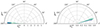Fig. 1. Representation of the parasitic wavevectors kh at t = 0 and at saturation, t = tsat, for all the runs in Table C.1. The initial modulus $k_{\mathrm{h}}^{\mathrm{ini}}$ ranges between 3 and 5, but the initial angle θini is very close to 180° in all cases. The wavevectors at saturation have almost the same angle θsat at around 18°, and the modulus $k_{\mathrm{h}}^{\mathrm{sat}}$ lies around 0.7.

3.2. Understanding the results

To shed light on the dynamics characterizing the behavior of the fastest growing parasites we examine in detail the evolution of some of the modes from run b0m-dh in Figs. 2, 3. We focus our attention on the mode that is first to reach the same amplitude as the MRI, that is to say, the fastest parasitic mode (red line); a mode that takes a bit longer to accomplish the same (yellow line), and a mode that grows initially but then stalls and later decays (blue line).

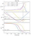Fig. 2. Top panel: time evolution of the averaged velocity, vPI, of three parasitic modes from the run b0m-dh: the fastest (red), another that saturates at later times (yellow), and one mode that does not saturate (blue). Middle panel: time evolution of the parasitic wavevector kh. Bottom panel: time evolution of the angle θ between the wavevector kh and the radial direction, $\check{\mathbf{x}}$. The modes start growing faster when kh and θ approach the values found in Pessah (2010), denoted as $k_{\mathrm{h}}^{\mathrm{P}10}$ and θP10, respectively.

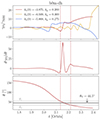Fig. 3. Top panel: time evolution of the normalized growth rate for the same modes as in Fig. 2. The growth rate stays considerably low up to a certain point, where it starts increasing to become more than ten times larger than the growth rate of the MRI (for the cases that reach saturation). Middle panel: evolution of the time derivative of γPI for the fastest mode. We draw vertical lines where the derivative takes positive values and at its last local maximum before saturation. Between these times, the parasitic mode grows the fastest. In the bottom panel, we show the evolution of the wavevector angle θ. We depict horizontal gray lines showing θ1 and θ2, i.e., the values of θ that indicate the fastest growth of the parasitic mode.

The top panel of Fig. 2 depicts the time evolution of the velocity computed from Eq. (31) for these three modes. The vertical velocity shear flow induced by the MRI is maximum in the direction given by θ_V. Examining the temporal evolution of k_h and θ is key to understanding why certain modes grow faster than others. The parasitic modes that can most effectively tap into this energy source, are those that, as their wavevectors are swept by the background flow according to Eq. (14), reach the direction θ_V with an optimal wavenumber. The velocity of the mode that does not saturate starts to decrease close to the time when its wavenumber k_h becomes larger than unity (middle panel). This seems in agreement with the results known from the time-independent calculations in Goodman & Xu (1994) and Pessah (2010) that show that parasitic modes with k_h > 1 do not grow. For the fastest growing mode (in red), θ starts decreasing before the slower mode (in yellow). This allows the fastest mode to start growing before the mode in yellow, when the MRI velocity is ∼10³ − 10⁴ times larger than the parasitic velocity, reaching values of θ ≈ θ^P10 = θ_V and $k_{\mathrm{h}}\approx k_{\mathrm{h}}^{\mathrm{P}10}=0.59$ (Pessah 2010) at earlier times. There is also a transient amplification of the parasitic velocity before the super-exponential growth that occurs when θ ≈ θ_V. This happens as the parasitic wavevector swings through from leading to trailing.

We showcase in Fig. 3 the time evolution of the growth rate of these PI modes (computed with Eq. (32)), normalized by the growth rate of the MRI from Eq. (9). The growth rate of the fastest mode starts increasing monotonically before the other mode that also saturates. Some modes reach a larger growth rate, but they saturate later because they get excited also later. The growth rate of the fastest growing mode starts increasing fast above 0 at t ≈ 2.15 orbits and then it continues growing at a slower rate. The middle panel shows the evolution of its time derivative. The region where the derivative takes positive values and increases faster coincides with values of θ (bottom panel) around θ_V = 44.5°. The rapid decrease of the derivative of the growth rate before the period of fast growth is due to the stabilizing effect of the MRI magnetic field, which is perpendicular to the MRI velocity field⁶. This behavior is also observed in the other cases from Table C.1, and also for other modes that saturate at later times (see also Fig. 6).

Figure 4 shows that the rapid increase of the parasitic modes coincides with the time-dependent wavevector k_h being aligned with the MRI velocity field. When the growth rate starts increasing monotonically at θ₁ (cf. Fig. 3), the direction of k_h is getting close to θ_V. The mode grows faster and its increase slows down when θ falls below θ_V. The angle θ₂ of Fig. 4 corresponds to the last turning point of the growth rate before saturation. The values of θ₁ and θ₂ are given by the vertical dashed lines of Fig. 3 (see also the horizontal gray lines in the bottom panel). The black solid lines for θ₁ and θ₂ correspond to the mean value of these angles from the runs of Table C.1, and the shaded regions in red depict the 1-σ deviation. As seen in Fig. 4, the values of θ₂ are almost the same for all runs, which means that, independently from the initial amplitude of the instabilities, the fastest parasitic modes start increasing at a reduced rate when θ ≳ 30°. Alternatively, there seems to be a larger dispersion for θ₁, with an average value of ${\overline{\theta }}_1\approx 60°$. Thus, the modes start their phase of super-exponential growth at an angle θ = θ₁ > θ_V. After the braking in the parasitic growth, the fastest mode eventually saturates. This result is consistent with the findings made by Pessah (2010), even though the saturation criterion is different. In Pessah (2010), the saturation occurs when the parasitic growth rate equals the MRI one, and our criterion is the one given in Eq. (29). When the parasitic amplitude reaches a similar value than the MRI channel’s, the parasitic growth rate is already several times larger than the MRI growth rate (see Fig. 3). Furthermore, with the current approach, it takes more time to the MRI to saturate, leading to a smaller θ^sat and larger $k_{\mathrm{h}}^{\mathrm{sat}}$. This is in agreement with the predictions from Latter et al. (2010), who stated that it should take more time to saturate due to the inclusion of the background shear in the equations and the time dependence of k_h.

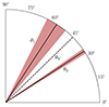Fig. 4. Values of the angle θ for which the PIs grow super-exponentially. The rapid increase of the secondary modes occurs between θ1 and θ2, depicted with solid black lines. These lines correspond to the mean value of these angles for the runs from Table C.1. The red-shaded regions represent the 1-σ deviation. The black dashed line stands for the direction of the MRI velocity field, θV = 44.5°.

4. An effective model for the amplification factor

Appealing to physical intuition and guided by our numerical results, we here seek to provide a simple expression for the amplification factor obtained when the fastest parasite, being advected by the background shear flow, is able to match the amplitude of the fastest, exponentially growing MRI mode.

In this Section, we employ a different value of the shear parameter, q = 1.25, instead of the Keplerian value (q = 1.5), in order to make a better comparison with the results from the numerical simulations of Rembiasz et al. (2016b), who use q = 1.25. We also consider the fastest MRI mode associated to this value of q. This mode is characterized by a vertical wavenumber K ≈ 0.93, angles θ_V = 45° and θ_B = 135°, and a ratio of MRI aplitudes V₀/B₀ ≈ 0.67. All these values are very similar to those for q = 1.5.

The analysis of the results presented in Table C.2 (employing q = 1.25) and illustrated in Fig. 5 reveals that the amplification factor is insensitive to the initial amplitude of the MRI mode while it may change by a factor of a few when the initial amplitude of the parasitic modes varies by a few orders of magnitude. The results from Table C.1 (using q = 1.5) are not depicted in Fig. 5, but are almost identical, meaning that the slight change in the shear parameter q does not have notable effects.

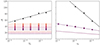Fig. 5. Left panel: dependence of the amplification factor, defined in Eq. (34), on the amplitude of the initial MRI velocity field, V0. Right panel: dependence of the amplification factor on the initial PI velocity field, v0. We use the runs from Table C.2 (solid lines with squares). Each color represents a different initial PI amplitude, v0, where the darker colors stand for larger values of v0. The solid lines represent the fit from Eq. (45). The dashed lines stand for the amplification factor computed with Eq. (42), i.e., assuming no background shear. The black triangles correspond to the results from the numerical simulations of Rembiasz et al. (2016b), and the black solid line is the linear fit from Eq. (47).

We can make use of this result to find an approximate expression for the amplification factor which is physically motivated. We proceed in two steps. First, we find the expression for the amplification factor ignoring the fact that the parasitic wavevector k_h is advected by the background shear. We account for this effect in a second step as described below.

4.1. Incorporating the exponential growth of the MRI

Building on the results presented in Pessah (2010), Rembiasz et al. (2016b) derived an approximate expression for the amplification factor assuming that the parasitic growth rate is given by

$$\begin{array}{c}\hfill {\gamma }_{\mathrm{PI}}^{\mathrm{P}10}=\sigma K{V}_0(t),\end{array}$$(39)

where σ = 0.27 (Pessah 2010) and considering that ${\gamma }_{\mathrm{PI}}^{\mathrm{P}10}\equiv \dot{v}(t)/v(t)$. This leads to an analytical expression for the velocity of the parasitic mode

$$\begin{array}{c}\hfill v(t)=v_{0}exp\left[\frac{\sigma K{V}_0}{{\gamma }_{\mathrm{MRI}}}(e^{{\gamma }_{\mathrm{MRI}}t}-1)\right].\end{array}$$(40)

Equating v(t_sat) = ϵV(t_sat), and using the parasitic velocity from Eq. (40), leads an analytical expression for the amplification factor (Rembiasz et al. 2016b)

$$\begin{array}{c}\hfill \mathcal{A}-\frac{1}{2\sigma }ln\mathcal{A}=\frac{1}{2\sigma }[-ln(v_0)+ln\left(ϵ\sqrt{\frac{4q}{4-q}}\right)]+\sqrt{\frac{4-q}{4q}}{V}_0.\end{array}$$(41)

This equation can be solved using the LambertW function (Corless et al. 1996), which has known asymptotic approximations (see, e.g., Latter 2016, for an application). However, we prefer approximating it to a simple analytical formula. It can be seen that the amplification factor scales with the logarithm of the initial parasitic amplitude and also linearly with the initial MRI amplitude. Since initially V₀ ≪ 1, the amplification factor should be almost independent of the initial MRI channel amplitude. This behavior is observed in Fig. 5 (left panel), and the linear dependence with the logarithm of the parasitic amplitude can be seen in the right panel. The logarithmic dependence in the parameters q and ϵ implies that these values do not strongly affect the amplification factor. Similarly, one could obtain an expression for the saturation time, t_sat, which can provide another interesting diagnostic.

On the left-hand side of Eq. (41) there is a term involving ln𝒜 that prevents us from finding a close solution for the amplification factor. However, as shown in Fig. 5, the spread in 𝒜 is not big, which means that ln𝒜 presents values around ≈3 − 4. Therefore, from our data, we can regard this term as roughly constant and employ its average value, $ln\overline{\mathcal{A}}\approx 3.7$. The resulting expression for the amplification factor is

$$\begin{array}{c}\hfill \mathcal{A}\simeq \frac{1}{2\sigma }[-ln(v_0)+ln\left(ϵ\sqrt{\frac{4q}{4-q}}\right)+ln\overline{\mathcal{A}}]+\sqrt{\frac{4-q}{4q}}{V}_0.\end{array}$$(42)

4.2. Incorporating the advection of parasitic modes

It can be seen in Fig. 5 that the expression from (42) underestimates 𝒜 by a factor ∼2, compared to our results (dashed lines with respect to solid lines). This can be understood by the fact that incorporating the advection of the parasitic wavevector k_h by the background shear effectively reduces the growth rate of the parasitic modes, as stated in Latter et al. (2010).

Using the results from our calculations, we can compute the factor, f, that needs to be applied to the parasitic growth rate from Eq. (39) in order to match the amplification factors obtained with our approach which included the background shear. Employing all the runs from Table C.2, we obtain that, on average, the factor needed is

$$\begin{array}{c}\hfill f=0.498\pm 0.006.\end{array}$$(43)

We note that the value of this fraction, f, is found by analyzing the parasitic modes that enable the breakdown of the primary MRI mode the fastest. The result is insensitive to the initial amplitudes of either the primary MRI or the secondary parasitic modes. The value we obtain agrees with the estimate made by Latter et al. (2010), who argued a reduction by a factor ≈2 by estimating the “average” growth rate during the time interval in which the parasites grow super-exponentially. This time interval is, in fact, short, because of the background disk shear. In our case, we aimed to apply a correcting factor to the parasitic growth rate from Eq. (39) to account for the background shear. We, therefore, equate the amplitude of the non-advected parasitic velocity from Eq. (40) near the primary MRI breakdown to the one obtained with the approach of this work (see Fig. 6). We found that the correcting factor f obtained in this way also leads to roughly similar growth rates at saturation time.

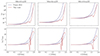Fig. 6. Top panels: time evolution of the parasitic velocity for different initial amplitudes of the PIs (from left to right, v0 = {0.112, 1.12, 11.2}×10−3) and a fixed initial MRI field, B0 = 3.33 × 10−2. The solid blue lines refer to the evolution of the parasitic velocity given in Eq. (40), whereas the red lines correspond to our approach. The dashed blue lines refer to the same velocity from Eq. (40), but adding the correcting factor f to the parasitic growth rate from Eq. (39). Bottom panels: time evolution of the normalized parasitic growth rate. Adding the correcting factor f to the expression from Eq. (39) (dashed blue lines), the parasitic growth rate roughly agrees with the one we obtain in our study (solid red lines).

The top panels in Fig. 6 depict the evolution of the parasitic velocity using Eq. (40) (solid blue line), using the same equation but introducing the factor f, so that ${\gamma }_{\mathrm{PI}}^{\mathrm{P}10}\to f{\gamma }_{\mathrm{PI}}^{\mathrm{P}10}$ in Eq. (39) (dashed blue line), and the actual evolution of a parasitic mode (solid red line) obtained from solving the initial value problem. As expected, the parasitic mode with a constant wavevector k_h aligned with the MRI velocity (solid blue curve), as implied by Eq. (40), grows faster than the parasitic modes whose wavevector is advected by the background shear flow (solid red curve). In the bottom panels we show the evolution of the normalized parasitic growth rate. By introducing the factor f from Eq. (43) in the analytical expression for the parasitic growth rate from Pessah (2010), the parasitic mode with constant wavevector k_h can reach the same amplitude as the parasitic mode with time-dependent wavevector advected by the background shear. Including this factor f in Eq. (39) in the amplification factor we obtain

$$\begin{array}{c}\hfill \mathcal{A}\simeq \frac{1}{2f\sigma }[-ln(v_0)+ln\left(ϵ\sqrt{\frac{4q}{4-q}}\right)+ln\overline{\mathcal{A}}],\end{array}$$(44)

where, supported by the results in Fig. 5, we neglect the dependence of 𝒜 on V₀.

4.3. An independent check using parasitic mode dynamics

Equation (44) has been obtained in a somewhat ad hoc way by bringing together various approximations without much regard for rigor. As an independent way to check whether the dependencies implied can accurately describe the results we obtained by solving for the full dynamical evolution of the parasites feeding off exponentially growing MRI modes while being advected by the background shear, we proceed as follows. Using the results from Tables C.1 and C.2, we seek to find the coefficients in the expression:

$$\begin{array}{c}\hfill \mathcal{A}\simeq \frac{1}{\sigma }[-b\prime ln(v_0)+c\prime (ln\left(ϵ\sqrt{\frac{4q}{4-q}}\right)+ln\overline{\mathcal{A}})].\end{array}$$(45)

Here, we consider ϵ = 1. Using the runs from Table C.1 (q = 1.5), we perform a linear fit and find that b′ = 1.022 ± 0.014 and c′ = 0.714 ± 0.019, with R² = 0.996. Alternatively, using the results from Table C.2 (q = 1.25), the coefficients are b′ = 1.038 ± 0.011 and c′ = 0.832 ± 0.019, and R² = 0.997. Both coefficients are, for both values of q, very close to unity, especially b′. The fact that c′ takes slightly smaller values than expected might be due to the term with $ln\overline{\mathcal{A}}$. In any case, the fact that all coefficients are order 𝒪(1) shows that the dependencies in Eq. (44) are indeed roughly correct.

4.4. A simple expression for the amplification factor

With all these considerations we can provide a simple expression that encapsulates the key processes involved and make use of the insights provided by our calculations to provide a reasonable accurate description of the amplification of the MRI as limited by the fastest parasitic modes as

$$\begin{array}{c}\hfill B_0(t_{\mathrm{sat}})\simeq \frac{{\overline{B}}_z}{0.135}[-ln(v_0)+ln\left(\sqrt{\frac{4q}{4-q}}\right)+3.7],\end{array}$$(46)

where ${\overline{B}}_z$ is the large-scale vertical magnetic field, v₀ is the initial amplitude of the parasitic mode, and q is the shear parameter.

5. Comparison with numerical simulations

5.1. Amplification factors

The role of PIs in the breakdown of the primary MRI mode has been studied through numerical simulations thoroughly during the last decade (Obergaulinger et al. 2009; Lesur & Longaretti 2011; Sorathia et al. 2012; Murphy & Pessah 2015; Rembiasz et al. 2016a; Hirai et al. 2018; Gogichaishvili et al. 2018). The use of numerical simulations has allowed the nonlinear regime of the MRI to be studied. However, numerical studies have not usually focused on addressing the role that seed perturbations, that excite unstable modes (either the MRI itself or the parasites) may play on the saturation level of the ensuing turbulence.

Rembiasz et al. (2016b) addressed this issue by carrying out shearing box simulations using the pseudo-spectral code SNOOPY (Lesur & Longaretti 2005, 2007) for different values of the initial amplitudes to seed the MRI, V₀, and the PIs, v₀. Figure 5 shows the amplification factors they obtained with black triangles. In the left panel, the initial parasitic amplitude is fixed at v₀ = 1.12 × 10⁻², whereas in the right panel the initial MRI velocity is fixed at V₀ = 2.2 × 10⁻³. Their results show a steeper dependence on the initial MRI velocity (left panel) and on the initial parasitic amplitudes (right panel). These trends are captured by the authors proposing that the amplification factor scales according to

$$\begin{array}{c}\hfill \mathcal{A}(V_0,v_0)=aln{V}_0+bln{v}_0+c,\end{array}$$(47)

where a = 5.4 ± 0.55, b = −20.2 ± 1.2, c = −101 ± 13. The value of the factor c differs from the one from the fit in Fig. 5 because the units employed in Rembiasz et al. (2016b) are different.

We attribute the discrepancy in the amplification factors we obtained with respect to those obtained in numerical simulations by Rembiasz et al. (2016b), shown in Fig. 5, to the different ways the modes involved are excited. We speculate, on rather reasonable grounds, that the larger amplification factors seen in numerical simulations could be due to the fact that the initial conditions do not seed directly the fastest modes involved. Rembiasz et al. (2016b) only excited the fastest growing velocity MRI field (letting the magnetic MRI field grow later), and they excited a large set of parasitic velocities applying random factors to their initial amplitudes. In our approach, only the fastest primary (MRI) and the secondary (parasitic) modes interact to reach saturation. The initial primary modes correspond to the fastest MRI eigenmode in Eq. (7). In addition, every time we seed secondary perturbations, we do so by exciting parasitic eigenmodes at the same initial time we allow the MRI mode to start evolving. Under these conditions, we define the amplitude of the MRI at saturation by equating the (kinetic) energy densities of the fastest MRI mode and the fastest parasitic mode. For initial conditions that exclusively involve perturbations in the velocity amplitude of the primary, V₀, it takes longer for the primary MRI mode, with the corresponding B₀, to emerge and grow exponentially at the fastest rate. This produces a delay in the onset of the secondary mode that grows to saturation, resulting in a higher amplitude for the MRI mode near breakdown that is higher than the one we would have obtained had the primary MRI mode been seeded directly. This may explain the trend exhibited by numerical results on the left panel of Fig. 5. Concerning the discrepancies observed in terms of the initial amplitude of the secondary perturbations, on the right panel of Fig. 5, it seems natural for saturation to be reached at a lower amplification when the fastest secondary mode is excited directly. This is because depositing the same amount of kinetic energy in a broad spectrum of secondary velocity perturbations is less efficient in seeding the parasites, allowing the primary to reach a higher amplitude.

It is worth mentioning that Rembiasz et al. (2016b) performed simulations with another numerical code, AENUS (Obergaulinger 2008), with different radial boundary conditions, physical assumptions and numerical schemes. The resulting amplification factor differed by a factor 5 from that obtained with the SNOOPY code (𝒜 ≈ 19 with AENUS instead of 𝒜 ≈ 90 with SNOOPY). Moreover, they found that employing a different form of the initial perturbations also changed the amplification factor, obtaining 𝒜 ≈ 60 instead of 𝒜 ≈ 90. Thus, differences in the simulation setup and the use of different numerical codes can have an impact on the amplification factor.

5.2. Other aspects

Numerical studies have also shown that the PIs eventually grow super-exponentially, reaching an amplitude comparable to the MRI and leading to a turbulent regime. It has also been found that, in the ideal MHD case, the fastest growing parasitic mode is aligned with the MRI velocity field (Rembiasz et al. 2016a; Hirai et al. 2018), which is in agreement with our findings. However, the parasitic wavenumbers at saturation found in numerical simulations (Rembiasz et al. 2016a; Hirai et al. 2018) are somewhat larger than those obtained here. This can be explained by the existence of other MRI modes (that grow more slowly), which results in a shear flow that is not purely sinusoidal. Moreover, the interaction of the PIs with the channels can cause the layered structure to become narrower, which induces a smaller parasitic mode just before the primary MRI mode breakdown (Hirai et al. 2018). These nonlinear effects are not captured by our approach.

Incorporating the advection of the parasitic modes has allowed us to understand that the modes that end up being able to reach amplitudes comparable to the MRI quite generically have initial horizontal wavelengths that are a factor of a few smaller than those previously inferred. We found that the fastest growth occurs when the parasitic wavevector is aligned with the MRI velocity field, in agreement with previous analytical and numerical studies. However, these modes must be properly resolved throughout their evolution in order for numerical simulations to capture their dynamics, and thus the MRI saturation, faithfully.

Using more than ten grid cells per wavelength is usually assumed to be enough to properly resolve the MRI (Rembiasz et al. 2016a). It is clear from our findings that it is equally important to resolve the evolution of the parasitic wavevector, as it is advected by the background shear flow. By performing box simulations with different aspect ratios and grid resolution, Rembiasz et al. (2016a) found that at least 60 zones per MRI channel are needed to obtain convergent results. This is due to the fact that the KH-type parasitic modes, triggered by the shear layer between MRI channels, develop finer spatial structures that need to be resolved. As a result, an initially leading wave with large (negative) k_x(0) may be numerically damped early on, and thus reach positive values of k_x(t) at a significantly lower amplitude than initially, which would complicate any estimate made from it. This issue can be explained by our results. The fastest parasitic modes have been found to be initially ∼3 − 5 times smaller than the MRI channels, meaning that an increased resolution in the horizontal plane might be needed to properly capture both the MRI and the PIs from the beginning of the simulation. If resolved, all the simulations with different numerical resolution should lead to the same amplification factor.

6. Summary, discussion, and implications

We have investigated the saturation of the MRI via parasitic modes relaxing important approximations previously invoked. This allowed us to obtain the most accurate calculation of the amplification factor to which the MRI can grow until the parasitic modes reach a comparable amplitude. To accomplish this, we carried out the first systematic analysis of the evolution of the PIs considering the temporal dependence that arises from the advection of the secondary parasitic modes feeding off exponentially growing primary MRI modes. Our approach involved solving a large number of initial value problems providing initial amplitudes for the modes involved. Even though the values for the initial amplitudes spanned several orders of magnitude we found that the amplification factor incurred by the MRI is remarkably robust, depending only logarithmically on the initial amplitude of the parasitic modes. This is overall in reasonable agreement, within a factor of two, with the amplification factors found in numerical simulations (e.g., Hawley et al. 1995; Obergaulinger et al. 2009; Murphy & Pessah 2015; Rembiasz et al. 2016a,b).

Building on previous work that has led to physical intuition on the processes involved in the breakdown of the primary MRI mode via PIs, and guided by our numerical results, we have provided a simple analytical expression in Eq. (46) that describes quite reasonably well the amplification of magnetic fields driven by the MRI.

The discrepancies with numerical studies mentioned above may highlight interesting issues with simulations. All in all, the amplification factors implied by our results differ by about a factor ≈2 from those reported in Rembiasz et al. (2016b). The slope on the right panel of Fig. 5 is also considerably larger than the one we obtain, although the trends are similar. The discrepancy between our results and those in Rembiasz et al. (2016b) can be partly explained by the different ways in which both the MRI and the parasites are excited in each of these settings (see Sect. 5 for a more detailed discussion). Another potential reason for which our predictions for saturation differ from numerical results may be because our approach does not capture the nonlinear interaction between primary and secondary that may arise near termination (see, e.g., Murphy & Pessah 2015; Gogichaishvili et al. 2018). In the nonlinear regime of the KH instability, a growth rate reduction is expected when the primary MRI mode breakdown approaches, so our predictions might underestimate the amplification factor (cf. Keppens et al. 1999; Obergaulinger et al. 2010). The plausible reasons we offer to explain the difference in amplification factors obtained via numerical simulations and via our approach can be explicitly tested by seeding numerical simulations exciting the fastest primary and secondaries.

In summary, with all the caveats stated, we have built an effective model to compute the saturation amplitude of the MRI, which differs up to a factor of roughly 2 from numerical results, which is smaller than the spread in the values provided by different codes using different initial conditions. This is the first approach that can achieve this and also highlights which parameters play the most relevant role in determining MRI saturation.

As shown in Eq. (33), the amplification factor is expressed in terms of the volume-averaged Maxwell stress tensor, ${\overline{\mathcal{M}}}_{\mathit{xy}}$. Thus, the effective model we have built here can be employed to predict the value at saturation of the turbulent stress tensors, since the Reynolds stress, ${\overline{\mathcal{R}}}_{\mathit{xy}}$, can be found via (Pessah et al. 2006a)

$$\begin{array}{c}\hfill {\overline{\mathcal{R}}}_{\mathit{xy}}=-\frac{q}{4-q}{\overline{\mathcal{M}}}_{\mathit{xy}}.\end{array}$$(48)

These components of the Maxwell and Reynolds stresses determine the radial flux of angular momentum via the total stress

$$\begin{array}{c}\hfill {\overline{\mathcal{T}}}_{\mathit{xy}}\equiv {\overline{\mathcal{R}}}_{\mathit{xy}}-{\overline{\mathcal{M}}}_{\mathit{xy}}.\end{array}$$(49)

Numerical simulations of astrophysical systems need to account for many physical processes (e.g., realistic equations of state, neutrino and radiative processes, etc.), usually limiting their spatial resolution. For this reason, and in order to resolve the initial field amplification due to the MRI, several works assume initial large-scale magnetic fields with unrealistically large magnitudes (e.g., Etienne et al. 2012; Gold et al. 2014; Ruiz et al. 2018, 2021; Bamber et al. 2024). Our effective model may be regarded as a means to predict the final magnetic field amplitude when secondary instabilities limit the MRI growth. This presents an alternative to invoking the large initial magnetic fields usually assumed in order to resolve the MRI.

Our findings may help develop more realistic effective models for MRI-driven turbulence to go beyond current approaches that employ effective viscosity terms (Fernández & Metzger 2013; Shibata et al. 2017; Fujibayashi et al. 2018, 2020; Radice 2020; Just et al. 2023), which are based on the alpha-viscosity prescription from Shakura & Sunyaev (1973). The resulting radial flux of the angular momentum (cf. Eq. (49)) can be used as a viscosity term in the momentum equation that allows transporting angular momentum at the correct rate even though the MRI is not well-resolved by the numerical simulation. The functional dependence of the effective model from Eq. (46) on the initial amplitudes of the modes and on the shear parameter q improves its adaptability to different disk conditions with respect to the widely used alpha-viscosity⁷. For example, the subgrid model presented in Miravet-Tenés et al. (2022) makes use of the findings made by Pessah (2010) to build evolution equations for the turbulent kinetic energy densities of both the MRI and PIs. This model can be improved by incorporating the findings of this work, namely, by including the factor f ≃ 1/2 from Eq. (43) in the parasitic growth rate that appears in these equations.

The effective model for MRI saturation we obtained can also be used to develop closure relations to link mean magnetic fields with turbulent stresses which are critical in models that go beyond viscous prescriptions for angular momentum transport (e.g., Kato & Yoshizawa 1993, 1995; Ogilvie 2003; Pessah et al. 2006b, 2008). This is a sensible approach, because even though nonlinear effects may result in some amplitude fluctuations during the turbulent state, the effective model presented here can provide an estimate of the average MRI amplitude after saturation (e.g., Rembiasz et al. 2016b; Hirai et al. 2018; Reboul-Salze et al. 2021).

The insights obtained in better understanding the saturation mechanism for the MRI have the potential to bring us a step closer to developing more realistic dynamical mean-field dynamo models where MRI-driven turbulence is naturally built-in (Gressel 2010; Gressel & Pessah 2015, 2022; Vourellis & Fendt 2021).

Acknowledgments

We thank Pablo Cerdá-Durán, José A. Font, Henrik Latter, George Mamatsashvili, Kaushik Satapathy, and Loren E. Held for helpful discussions and useful comments. We also thank the referee for a comprehensive and useful report that helped us improve the manuscript. MMT acknowledges support from the Ministerio de Ciencia, Innovación y Universidades del Gobierno de España through the “Ayuda para la Formación de Profesorado Universitario” (FPU) fellowship No. FPU19/01750 and the “Ayuda FPU Complementaria de Movilidad para Estancias Breves en Centros Extranjeros” fellowship No. EST23/00420, from the Spanish Agencia Estatal de Investigación (grant PID2021-125485NB-C21) funded by MCIN/AEI/10.13039/501100011033 and ERDF A way of making Europe, and from the Science and Technology Facilities Council (STFC), via grant No. ST/Y000811/1. MEP gratefully acknowledges support from the Independent Research Fund Denmark via grant ID 10.46540/3103-00205B. This work has used the following open-source packages: NUMPY (Harris et al. 2020), SCIPY (Virtanen et al. 2020) and MATPLOTLIB (Hunter 2007).

References

Appendix A: Evolving the system of equations for the parasitic instabilities

Having obtained the initial values of the Fourier amplitudes of the velocity and magnetic fields of the PIs, we can evolve the system of Eqs. (21) and (22). To accomplish this we write it in vector form as

$$\begin{array}{c}\hfill {\partial }_t\mathit{x}(t)=\mathit{A}(t)\mathit{x}(t),\end{array}$$(A.1)

where the vectors x contain the Fourier amplitudes α_n(t) and β_n(t) and A(t) is the matrix of coefficients. This coupled linear differential equation system can be decoupled, and solved, as follows.

Let the matrix A(t) be expressed in terms of a diagonal matrix, Λ(t):

$$\begin{array}{c}\hfill \mathbf{\Lambda }={\mathit{S}}^{-1}\mathit{A}\mathit{S},\end{array}$$(A.2)

where S is a matrix built with the eigenvectors of A(t) as columns and Λ is a diagonal matrix with the eigenvalues of A as elements. The equations of motion (A.1) can be written in terms of the variable

$$\begin{array}{c}\hfill \mathit{\eta }={\mathit{S}}^{-1}\mathit{x},\end{array}$$(A.3)

as a set of decoupled equations

$$\begin{array}{c}\hfill {\partial }_t\mathit{\eta }(t)=\mathbf{\Lambda }\mathit{\eta }(t),\end{array}$$(A.4)

which can be cast independently for each component

$$\begin{array}{c}\hfill {\partial }_t{\eta }_i={\lambda }_i{\eta }_i.\end{array}$$(A.5)

This is valid only when S ≠ S(t), and we assume this is the case in a small enough time interval Δt. The solutions can now be trivially obtained as

$$\begin{array}{c}\hfill {\eta }_i(t)=exp\left[{\displaystyle {\int }_{t-\mathrm{\Delta }t}^t}{\lambda }_i(\tau )d\tau \right]{\eta }_i(t-\mathrm{\Delta }t).\end{array}$$(A.6)

We can define the matrix composed of elements given by the right-hand-side of the above equation:

$$\begin{array}{c}\hfill E_{\mathit{ij}}\equiv {\delta }_{\mathit{ij}}exp\left[{\displaystyle {\int }_{t-\mathrm{\Delta }t}^t}{\lambda }_i(\tau )d\tau \right].\end{array}$$(A.7)

For small enough time intervals Δt, we can assume that λ_i are constant⁸ to obtain

$$\begin{array}{c}\hfill E_{\mathit{ij}}\approx {\delta }_{\mathit{ij}}{e}^{\mathrm{\Delta }t{\lambda }_i}.\end{array}$$(A.8)

In terms of the matrix E, the solutions we seek satisfy

$$\begin{array}{c}\hfill \mathit{x}(t)=\mathit{S}\mathit{E}{\mathit{S}}^{-1}\mathit{x}(t-\mathrm{\Delta }t).\end{array}$$(A.9)

In solving the equations given by (A.4), we employ the approach shown in Eq. (A.8) using an adaptive timestep Δt that decreases as γ_PI increases, as shown in Table A.1. The initial timestep is set to Δt₀ = 0.1.

Appendix B: Physical structure of the parasitic modes

To study the structure of the parasitic modes and the disruption of the MRI channels, we calculate the components of the vorticity and current density perpendicular to the plane (${\stackrel{\mathbf{ˇ}}{\mathit{k}}}_{\mathbf{h}},\check{\mathbf{z}}$):

$$\begin{array}{cc}\hfill \delta {\omega }_{\perp }(t;\mathit{x})& =(\mathbf{\nabla }\mathbf{\times }\mathit{v})·{\stackrel{\mathbf{ˇ}}{\mathit{k}}}_{\mathbf{p}},\hfill \end{array}$$(B.1)

$$\begin{array}{cc}\hfill \delta j_{\perp }(t;\mathit{x})& =(\mathbf{\nabla }\mathbf{\times }\mathit{b})·{\stackrel{\mathbf{ˇ}}{\mathit{k}}}_{\mathbf{p}},\hfill \end{array}$$(B.2)

where ${\stackrel{\mathbf{ˇ}}{\mathit{k}}}_{\mathbf{p}}$ is the direction perpendicular to (${\stackrel{\mathbf{ˇ}}{\mathit{k}}}_{\mathbf{h}},\check{\mathbf{z}}$): ${\stackrel{\mathbf{ˇ}}{\mathit{k}}}_{\mathbf{p}}\equiv \check{\mathbf{z}}\wedge {\stackrel{\mathbf{ˇ}}{\mathit{k}}}_{\mathbf{h}}$. Using Eqs. (27) and (28), we obtain

$$\begin{array}{cc}\hfill \delta {\omega }_{\perp }(t;\mathit{x})& =-\frac{i}{k_{\mathrm{h}}}{\displaystyle \sum _{n=-\infty }^{\infty }}[k_{\mathrm{h}}^2+{(n+k_z)}^2]{\alpha }_n(t)e^{i(n+k_z)z}{e}^{i{k}_{\mathrm{h}}h},\hfill \end{array}$$(B.3)

$$\begin{array}{cc}\hfill \delta j_{\perp }(t;\mathit{x})& =-\frac{i}{k_{\mathrm{h}}}{\displaystyle \sum _{n=-\infty }^{\infty }}[k_{\mathrm{h}}^2+{(n+k_z)}^2]{\beta }_n(t)e^{i(n+k_z)z}{e}^{i{k}_{\mathrm{h}}h},\hfill \end{array}$$(B.4)

where k_hh = k_h ⋅ x. The total vorticity and current can be obtained by adding the contribution from the MRI fields projected onto the direction ${\stackrel{\mathbf{ˇ}}{\mathit{k}}}_{\mathbf{h}}$:

$$\begin{array}{cc}\hfill {\omega }_{\perp }(t;\mathit{x})& =V_0(t)cos(Kz)cos(\theta -{\theta }_{\mathrm{V}})+\delta {\omega }_{\perp }(t;\mathit{x}),\hfill \end{array}$$(B.5)

$$\begin{array}{cc}\hfill j_{\perp }(t;\mathit{x})& =-B_0(t)sin(Kz)cos(\theta -{\theta }_{\mathrm{B}})+\delta j_{\perp }(t;\mathit{x}).\hfill \end{array}$$(B.6)

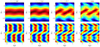Fig. B.1. Physical structure of the fastest parasitic modes, including the velocity field of the primary MRI mode, for different times (in terms of the number of orbits, increasing from left to right). The arrows in the top and bottom panels correspond, respectively, to the projections of the total velocity, V(z)+v(h, z), and the parasitic velocity, v(h, z), onto the time-dependent plane (${\stackrel{\mathbf{ˇ}}{\mathit{k}}}_{\mathbf{h}},\check{\mathbf{z}}$). The color contours correspond to the associated total vorticity ω⊥ and the parasitic vorticity δω⊥ projected onto the direction perpendicular to ${\stackrel{\mathbf{ˇ}}{\mathit{k}}}_{\mathbf{h}}$.

Fig. B.2. Same as Fig. B.1, but including the magnetic and the current density fields instead of the velocity and the vorticity, respectively.

In Fig. B.1 we depict the total vorticity field ω_⊥ projected onto the plane (${\stackrel{\mathbf{ˇ}}{\mathit{k}}}_{\mathbf{h}},\check{\mathbf{z}}$), where the arrows represent the total velocity V + v (top panels) and the vorticity of the parasitic mode δω_⊥ with the velocity field v (bottom panels), for different times. At early times (first panel), the MRI channels remain steady, since the fastest parasitic mode has not reached enough amplitude yet. When the primary MRI mode breakdown approaches (last three panels), the channels are disrupted by the parasitic mode, showing the familiar wave-like structure expected from KH instability modes in a periodic background. The bottom panels representing the vorticity and velocity fields of the parasitic mode show a periodic structure of equidistant vortex sheets, similar to those in Fig. 8 in Pessah (2010), but gradually evolving to more elongated structures.

Alternatively, Fig. B.2 shows the current density and magnetic fields instead of the vorticity and the velocity fields. The magnetic parasitic field again forms periodic vortex sheets that become horizontally elongated as saturation approaches. The MRI channels get disrupted and adopt the same structure as shown in Fig. 10 from Pessah (2010).

Appendix C: Summary of the evolution runs for the parasitic modes

We provide tables listing the parameters and important properties of the fastest parasitic modes evolved in this work:

• Table C.1 summarizes several properties of the fastest growing parasitic modes at t = 0 and at saturation time, t_sat, for different initial amplitudes of primary MRI and secondary modes. The shear factor used for these runs is q = 1.5.

• Table C.2 shows the same quantities as Table C.1, but the value of the shear parameter corresponds to q = 1.25, and different initial amplitudes are also used.

All Tables

All Figures

Fig. 1. Representation of the parasitic wavevectors kh at t = 0 and at saturation, t = tsat, for all the runs in Table C.1. The initial modulus $k_{\mathrm{h}}^{\mathrm{ini}}$ ranges between 3 and 5, but the initial angle θini is very close to 180° in all cases. The wavevectors at saturation have almost the same angle θsat at around 18°, and the modulus $k_{\mathrm{h}}^{\mathrm{sat}}$ lies around 0.7.

In the text

Fig. 2. Top panel: time evolution of the averaged velocity, vPI, of three parasitic modes from the run b0m-dh: the fastest (red), another that saturates at later times (yellow), and one mode that does not saturate (blue). Middle panel: time evolution of the parasitic wavevector kh. Bottom panel: time evolution of the angle θ between the wavevector kh and the radial direction, $\check{\mathbf{x}}$. The modes start growing faster when kh and θ approach the values found in Pessah (2010), denoted as $k_{\mathrm{h}}^{\mathrm{P}10}$ and θP10, respectively.

In the text

Fig. 3. Top panel: time evolution of the normalized growth rate for the same modes as in Fig. 2. The growth rate stays considerably low up to a certain point, where it starts increasing to become more than ten times larger than the growth rate of the MRI (for the cases that reach saturation). Middle panel: evolution of the time derivative of γPI for the fastest mode. We draw vertical lines where the derivative takes positive values and at its last local maximum before saturation. Between these times, the parasitic mode grows the fastest. In the bottom panel, we show the evolution of the wavevector angle θ. We depict horizontal gray lines showing θ1 and θ2, i.e., the values of θ that indicate the fastest growth of the parasitic mode.

In the text

	Fig. 4. Values of the angle θ for which the PIs grow super-exponentially. The rapid increase of the secondary modes occurs between θ1 and θ2, depicted with solid black lines. These lines correspond to the mean value of these angles for the runs from Table C.1. The red-shaded regions represent the 1-σ deviation. The black dashed line stands for the direction of the MRI velocity field, θV = 44.5°.
In the text

Fig. 5. Left panel: dependence of the amplification factor, defined in Eq. (34), on the amplitude of the initial MRI velocity field, V0. Right panel: dependence of the amplification factor on the initial PI velocity field, v0. We use the runs from Table C.2 (solid lines with squares). Each color represents a different initial PI amplitude, v0, where the darker colors stand for larger values of v0. The solid lines represent the fit from Eq. (45). The dashed lines stand for the amplification factor computed with Eq. (42), i.e., assuming no background shear. The black triangles correspond to the results from the numerical simulations of Rembiasz et al. (2016b), and the black solid line is the linear fit from Eq. (47).

In the text

Fig. 6. Top panels: time evolution of the parasitic velocity for different initial amplitudes of the PIs (from left to right, v0 = {0.112, 1.12, 11.2}×10−3) and a fixed initial MRI field, B0 = 3.33 × 10−2. The solid blue lines refer to the evolution of the parasitic velocity given in Eq. (40), whereas the red lines correspond to our approach. The dashed blue lines refer to the same velocity from Eq. (40), but adding the correcting factor f to the parasitic growth rate from Eq. (39). Bottom panels: time evolution of the normalized parasitic growth rate. Adding the correcting factor f to the expression from Eq. (39) (dashed blue lines), the parasitic growth rate roughly agrees with the one we obtain in our study (solid red lines).

In the text

Fig. B.1. Physical structure of the fastest parasitic modes, including the velocity field of the primary MRI mode, for different times (in terms of the number of orbits, increasing from left to right). The arrows in the top and bottom panels correspond, respectively, to the projections of the total velocity, V(z)+v(h, z), and the parasitic velocity, v(h, z), onto the time-dependent plane (${\stackrel{\mathbf{ˇ}}{\mathit{k}}}_{\mathbf{h}},\check{\mathbf{z}}$). The color contours correspond to the associated total vorticity ω⊥ and the parasitic vorticity δω⊥ projected onto the direction perpendicular to ${\stackrel{\mathbf{ˇ}}{\mathit{k}}}_{\mathbf{h}}$.

In the text

	Fig. B.2. Same as Fig. B.1, but including the magnetic and the current density fields instead of the velocity and the vorticity, respectively.
In the text

References

- Akiyama, S., Wheeler, J. C., Meier, D. L., & Lichtenstadt, I. 2003, ApJ, 584, 954 [NASA ADS] [CrossRef] [Google Scholar]
- Balbus, S. A., & Hawley, J. F. 1991, ApJ, 376, 214 [Google Scholar]
- Balbus, S. A., & Hawley, J. F. 1992, ApJ, 400, 610 [CrossRef] [Google Scholar]
- Balbus, S. A., & Hawley, J. F. 1998, Rev. Mod. Phys., 70, 1 [Google Scholar]
- Bamber, J., Tsokaros, A., Ruiz, M., & Shapiro, S. L. 2024, Phys. Rev. D, 110, 024046 [NASA ADS] [Google Scholar]
- Brandenburg, A., Nordlund, A., Stein, R. F., & Torkelsson, U. 1995, ApJ, 446, 741 [NASA ADS] [CrossRef] [Google Scholar]
- Brughmans, N., Keppens, R., & Goedbloed, H. 2024, ApJ, 968, 19 [NASA ADS] [Google Scholar]
- Cerdá-Durán, P., Font, J. A., Antón, L., & Müller, E. 2008, A&A, 492, 937 [NASA ADS] [CrossRef] [EDP Sciences] [Google Scholar]
- Chandrasekhar, S. 1960, Proc. Natl. Acad. Sci., 46, 253 [NASA ADS] [CrossRef] [Google Scholar]
- Christie, I. M., Lalakos, A., Tchekhovskoy, A., et al. 2019, MNRAS, 490, 4811 [NASA ADS] [CrossRef] [Google Scholar]
- Combi, L., & Siegel, D. M. 2023, Phys. Rev. Lett., 131, 231402 [Google Scholar]
- Corless, R. M., Gonnet, G. H., Hare, D. E. G., Jeffrey, D. J., & Knuth, D. E. 1996, Adv. Comput. Math., 5, 329 [CrossRef] [Google Scholar]
- Das, U., Begelman, M. C., & Lesur, G. 2018, MNRAS, 473, 2791 [NASA ADS] [CrossRef] [Google Scholar]
- Davis, S. W., Stone, J. M., & Pessah, M. E. 2010, ApJ, 713, 52 [NASA ADS] [CrossRef] [Google Scholar]
- Duez, M. D., Liu, Y. T., Shapiro, S. L., Shibata, M., & Stephens, B. C. 2006a, Phys. Rev. Lett., 96, 031101 [Google Scholar]
- Duez, M. D., Liu, Y. T., Shapiro, S. L., Shibata, M., & Stephens, B. C. 2006b, Phys. Rev. D, 73, 104015 [NASA ADS] [Google Scholar]
- Etienne, Z. B., Liu, Y. T., Paschalidis, V., & Shapiro, S. L. 2012, Phys. Rev. D, 85, 064029 [Google Scholar]
- Fernández, R., & Metzger, B. D. 2013, MNRAS, 435, 502 [CrossRef] [Google Scholar]
- Fernández, R., Tchekhovskoy, A., Quataert, E., Foucart, F., & Kasen, D. 2019, MNRAS, 482, 3373 [CrossRef] [Google Scholar]
- Fleming, T. P., Stone, J. M., & Hawley, J. F. 2000, ApJ, 530, 464 [Google Scholar]
- Fujibayashi, S., Kiuchi, K., Nishimura, N., Sekiguchi, Y., & Shibata, M. 2018, ApJ, 860, 64 [NASA ADS] [CrossRef] [Google Scholar]
- Fujibayashi, S., Shibata, M., Wanajo, S., et al. 2020, Phys. Rev. D, 101, 083029 [Google Scholar]
- Gardiner, T. A., & Stone, J. M. 2005, in Magnetic Fields in the Universe: From Laboratory and Stars to Primordial Structures, eds. E. M. de Gouveia dal Pino, G. Lugones, & A. Lazarian (AIP), AIP Conf. Ser., 784, 475 [Google Scholar]
- Gogichaishvili, D., Mamatsashvili, G., Horton, W., & Chagelishvili, G. 2018, ApJ, 866, 134 [Google Scholar]
- Gold, R., Paschalidis, V., Etienne, Z. B., Shapiro, S. L., & Pfeiffer, H. P. 2014, Phys. Rev. D, 89, 064060 [NASA ADS] [CrossRef] [Google Scholar]
- Goodman, J., & Xu, G. 1994, ApJ, 432, 213 [NASA ADS] [CrossRef] [Google Scholar]
- Gressel, O. 2010, MNRAS, 405, 41 [NASA ADS] [CrossRef] [Google Scholar]
- Gressel, O., & Pessah, M. E. 2015, ApJ, 810, 59 [NASA ADS] [CrossRef] [Google Scholar]
- Gressel, O., & Pessah, M. E. 2022, ApJ, 928, 118 [Google Scholar]
- Harris, C. R., Millman, K. J., van der Walt, S. J., et al. 2020, Nature, 585, 357 [NASA ADS] [CrossRef] [Google Scholar]
- Hawley, J. F., Gammie, C. F., & Balbus, S. A. 1995, ApJ, 440, 742 [Google Scholar]
- Hawley, J. F., Guan, X., & Krolik, J. H. 2011, ApJ, 738, 84 [NASA ADS] [CrossRef] [Google Scholar]
- Held, L. E., & Mamatsashvili, G. 2022, MNRAS, 517, 2309 [NASA ADS] [Google Scholar]
- Held, L. E., Mamatsashvili, G., & Pessah, M. E. 2024, MNRAS, 530, 2232 [NASA ADS] [CrossRef] [Google Scholar]
- Hirai, K., Katoh, Y., Terada, N., & Kawai, S. 2018, ApJ, 853, 174 [Google Scholar]
- Hunter, J. D. 2007, Comput. Sci. Eng., 9, 90 [NASA ADS] [CrossRef] [Google Scholar]
- Johansen, A., & Levin, Y. 2008, A&A, 490, 501 [NASA ADS] [CrossRef] [EDP Sciences] [Google Scholar]
- Just, O., Vijayan, V., Xiong, Z., et al. 2023, ApJ, 951, L12 [NASA ADS] [CrossRef] [Google Scholar]
- Kato, S., & Yoshizawa, A. 1993, PASJ, 45, 103 [NASA ADS] [Google Scholar]
- Kato, S., & Yoshizawa, A. 1995, PASJ, 47, 629 [NASA ADS] [Google Scholar]
- Keppens, R., Tóth, G., Westermann, R. H. J., & Goedbloed, J. P. 1999, J. Plasma Phys., 61, 1 [NASA ADS] [CrossRef] [Google Scholar]
- Kiuchi, K., Sekiguchi, Y., Kyutoku, K., et al. 2015, Phys. Rev. D, 92, 064034 [Google Scholar]
- Kiuchi, K., Kyutoku, K., Sekiguchi, Y., & Shibata, M. 2018, Phys. Rev. D, 97, 124039 [NASA ADS] [CrossRef] [Google Scholar]
- Kiuchi, K., Reboul-Salze, A., Shibata, M., & Sekiguchi, Y. 2024, Nat. Astron., 8, 298 [Google Scholar]
- Latter, H. N. 2016, MNRAS, 455, 2608 [NASA ADS] [CrossRef] [Google Scholar]
- Latter, H. N., Lesaffre, P., & Balbus, S. A. 2009, MNRAS, 394, 715 [NASA ADS] [CrossRef] [Google Scholar]
- Latter, H. N., Fromang, S., & Gressel, O. 2010, MNRAS, 406, 848 [NASA ADS] [Google Scholar]
- Lesaffre, P., Balbus, S. A., & Latter, H. 2009, MNRAS, 396, 779 [NASA ADS] [CrossRef] [Google Scholar]
- Lesur, G., & Longaretti, P. Y. 2005, A&A, 444, 25 [NASA ADS] [CrossRef] [EDP Sciences] [Google Scholar]
- Lesur, G., & Longaretti, P. Y. 2007, MNRAS, 378, 1471 [NASA ADS] [CrossRef] [Google Scholar]
- Lesur, G., & Longaretti, P. Y. 2011, A&A, 528, A17 [NASA ADS] [CrossRef] [EDP Sciences] [Google Scholar]
- Longaretti, P. Y., & Lesur, G. 2010, A&A, 516, A51 [NASA ADS] [CrossRef] [EDP Sciences] [Google Scholar]
- Lynden-Bell, D., & Pringle, J. E. 1974, MNRAS, 168, 603 [Google Scholar]
- Mamatsashvili, G. R., Chagelishvili, G. D., Bodo, G., & Rossi, P. 2013, MNRAS, 435, 2552 [CrossRef] [Google Scholar]
- Mamatsashvili, G., Chagelishvili, G., Pessah, M. E., Stefani, F., & Bodo, G. 2020, ApJ, 904, 47 [NASA ADS] [CrossRef] [Google Scholar]
- Miravet-Tenés, M., Cerdá-Durán, P., Obergaulinger, M., & Font, J. A. 2022, MNRAS, 517, 3505 [Google Scholar]
- Mösta, P., Ott, C. D., Radice, D., et al. 2015, Nature, 528, 376 [CrossRef] [Google Scholar]
- Murphy, G. C., & Pessah, M. E. 2015, ApJ, 802, 139 [Google Scholar]
- Obergaulinger, M. 2008, Ph.D. Thesis, Max-Planck-Institute for Astrophysics, Garching, Germany [Google Scholar]
- Obergaulinger, M., Aloy, M. A., Dimmelmeier, H., & Müller, E. 2006, A&A, 457, 209 [NASA ADS] [CrossRef] [EDP Sciences] [Google Scholar]
- Obergaulinger, M., Cerdá-Durán, P., Müller, E., & Aloy, M. A. 2009, A&A, 498, 241 [NASA ADS] [CrossRef] [EDP Sciences] [Google Scholar]
- Obergaulinger, M., Aloy, M. A., & Müller, E. 2010, A&A, 515, A30 [NASA ADS] [CrossRef] [EDP Sciences] [Google Scholar]
- Ogilvie, G. I. 2003, MNRAS, 340, 969 [CrossRef] [Google Scholar]
- Paschalidis, V., Ruiz, M., & Shapiro, S. L. 2015, ApJ, 806, L14 [NASA ADS] [CrossRef] [Google Scholar]
- Pessah, M. E. 2010, ApJ, 716, 1012 [NASA ADS] [CrossRef] [Google Scholar]
- Pessah, M. E., & Chan, C.-K. 2008, ApJ, 684, 498 [NASA ADS] [CrossRef] [Google Scholar]
- Pessah, M. E., & Chan, C.-K. 2012, ApJ, 751, 48 [Google Scholar]
- Pessah, M. E., & Goodman, J. 2009, ApJ, 698, L72 [NASA ADS] [CrossRef] [Google Scholar]
- Pessah, M. E., & Psaltis, D. 2005, ApJ, 628, 879 [NASA ADS] [CrossRef] [Google Scholar]
- Pessah, M. E., Chan, C.-K., & Psaltis, D. 2006a, MNRAS, 372, 183 [NASA ADS] [CrossRef] [Google Scholar]
- Pessah, M. E., Chan, C.-K., & Psaltis, D. 2006b, Phys. Rev. Lett., 97, 221103 [Google Scholar]
- Pessah, M. E., Chan, C.-K., & Psaltis, D. 2007, ApJ, 668, L51 [Google Scholar]
- Pessah, M. E., Chan, C.-K., & Psaltis, D. 2008, MNRAS, 383, 683 [Google Scholar]
- Radice, D. 2020, Symmetry, 12, 1249 [Google Scholar]
- Reboul-Salze, A., Guilet, J., Raynaud, R., & Bugli, M. 2021, A&A, 645, A109 [NASA ADS] [CrossRef] [EDP Sciences] [Google Scholar]
- Reboul-Salze, A., Guilet, J., Raynaud, R., & Bugli, M. 2022, A&A, 667, A94 [NASA ADS] [CrossRef] [EDP Sciences] [Google Scholar]
- Rembiasz, T., Obergaulinger, M., Cerdá-Durán, P., Müller, E., & Aloy, M. A. 2016a, MNRAS, 456, 3782 [NASA ADS] [CrossRef] [Google Scholar]
- Rembiasz, T., Guilet, J., Obergaulinger, M., et al. 2016b, MNRAS, 460, 3316 [NASA ADS] [CrossRef] [Google Scholar]
- Rezzolla, L., Giacomazzo, B., Baiotti, L., et al. 2011, ApJ, 732, L6 [NASA ADS] [CrossRef] [Google Scholar]
- Ruiz, M., Lang, R. N., Paschalidis, V., & Shapiro, S. L. 2016, ApJ, 824, L6 [NASA ADS] [CrossRef] [Google Scholar]
- Ruiz, M., Shapiro, S. L., & Tsokaros, A. 2018, Phys. Rev. D, 98, 123017 [NASA ADS] [CrossRef] [Google Scholar]
- Ruiz, M., Shapiro, S. L., & Tsokaros, A. 2021, Front. Astron. Space Sci., 8, 39 [Google Scholar]
- Sano, T., & Inutsuka, S.-I. 2001, ApJ, 561, L179 [Google Scholar]
- Sano, T., Inutsuka, S.-I., Turner, N. J., & Stone, J. M. 2004, ApJ, 605, 321 [NASA ADS] [CrossRef] [Google Scholar]
- Shakura, N. I., & Sunyaev, R. A. 1973, A&A, 24, 337 [NASA ADS] [Google Scholar]
- Shibata, M., Kiuchi, K., & Sekiguchi, Y.-I. 2017, Phys. Rev. D, 95, 083005 [NASA ADS] [CrossRef] [Google Scholar]
- Shibata, M., Fujibayashi, S., & Sekiguchi, Y. 2021, Phys. Rev. D, 104, 063026 [NASA ADS] [CrossRef] [Google Scholar]
- Siegel, D. M., Ciolfi, R., Harte, A. I., & Rezzolla, L. 2013, Phys. Rev. D, 87, 121302 [NASA ADS] [CrossRef] [Google Scholar]
- Sorathia, K. A., Reynolds, C. S., & Armitage, P. J. 2010, ApJ, 712, 1241 [Google Scholar]
- Sorathia, K. A., Reynolds, C. S., Stone, J. M., & Beckwith, K. 2012, ApJ, 749, 189 [NASA ADS] [CrossRef] [Google Scholar]
- Squire, J., Quataert, E., & Hopkins, P. F. 2024, ArXiv e-prints [arXiv:2409.05467] [Google Scholar]
- Velikhov, E. P. 1959, Soviet J. Exp. Theor. Phys., 9, 995 [Google Scholar]
- Virtanen, P., Gommers, R., Oliphant, T. E., et al. 2020, Nat. Methods, 17, 261 [Google Scholar]
- Vishniac, E. T. 2009, ApJ, 696, 1021 [NASA ADS] [CrossRef] [Google Scholar]
- Vourellis, C., & Fendt, C. 2021, ApJ, 911, 85 [NASA ADS] [CrossRef] [Google Scholar]