| Issue |
A&A
Volume 696, April 2025
|
|
|---|---|---|
| Article Number | A83 | |
| Number of page(s) | 9 | |
| Section | Extragalactic astronomy | |
| DOI | https://doi.org/10.1051/0004-6361/202452652 | |
| Published online | 07 April 2025 | |
Deep kiloparsec view of the molecular gas in a massive star-forming galaxy at cosmic noon
1
Departamento de Astronomía, Universidad de Concepción, Barrio Universitario, Concepción, Chile
2
Millenium Nucleus for Galaxies (MINGAL), Concepción, Chile
3
Max-Planck-Institut für Extraterrestische Physik, Giessenbachstr. 1, 85748 Garching, Germany
4
Cosmic Dawn Center (DAWN), Copenhagen, Denmark
5
DTU-Space, Technical University of Denmark, Elektrovej 327, DK-2800 Kgs. Lyngby, Denmark
6
Department of Astronomy, University of Maryland, College Park, MD 20742, USA
7
Purple Mountain Observatory, Chinese Academy of Sciences, 10 Yuanhua Road, Nanjing 210023, People’s Republic of China
8
INAF – Osservatorio Astronomico di Padova, Vicolo dell’Osservatorio 5, I-35122 Padova, Italy
⋆ Corresponding author; This email address is being protected from spambots. You need JavaScript enabled to view it.
Received:
17
October
2024
Accepted:
13
February
2025
Abstract
We present deep (∼20 hr), high-angular resolution Atacama Large Millimeter/submillimeter Array (ALMA) observations of the CO (4 − 3) and [CI] (1 − 0) transitions, along with the rest-frame 630 μm dust continuum, in BX610–a massive, main-sequence galaxy at the peak epoch of cosmic star formation (z = 2.21). Combined with deep Very Large Telescope (VLT) SINFONI observations of the Hα line, we characterize the molecular gas and star formation activity on kiloparsec scales. Our analysis reveals that the excitation of the molecular gas, as traced by the L′CO(4−3)/L′[CI](1−0) line luminosity ratio, decreases with increasing galactocentric radius. While the line luminosity ratios in the outskirts are similar to those typically found in main-sequence galaxies at z ∼ 1, the ratios in the central regions of BX610 are comparable to those observed in local starbursts. There is also a giant extra-nuclear star-forming clump in the southwest of BX610 that exhibits high star formation activity, molecular gas abundance, and molecular gas excitation. Furthermore, the central region of BX610 is rich in molecular gas (Mmol/M⋆ ≈ 1); however, at the current level of star formation activity, such molecular gas is expected to be depleted in ∼450 Myr. This, along with recent evidence for rapid inflow toward the center, suggests that BX610 may be experiencing an evolutionary phase often referred to as wet compaction, which is expected to lead to central gas depletion and subsequent inside-out quenching of star formation activity.
Key words: galaxies: evolution / galaxies: high-redshift / galaxies: ISM / galaxies: star formation
© The Authors 2025
 Open Access article, published by EDP Sciences, under the terms of the Creative Commons Attribution License (https://creativecommons.org/licenses/by/4.0), which permits unrestricted use, distribution, and reproduction in any medium, provided the original work is properly cited.
This article is published in open access under the Subscribe to Open model. This email address is being protected from spambots. You need JavaScript enabled to view it. to support open access publication.
1. Introduction
The epoch known as cosmic noon, when the Universe was ∼2–3 Gyr old, represents the peak of the cosmic star formation rate (SFR) density (e.g., Madau & Dickinson 2014), making it a critical period for studying galaxy evolution. Recent galaxy surveys have shown that the increased star formation activity during this time was primarily driven by abundant reservoirs of cold molecular gas, the fuel for star formation (e.g., Tacconi et al. 2018; Walter et al. 2020; Tacconi et al. 2020). Notably, the molecular gas fraction in massive star-forming galaxies (M⋆ ≳ 1010.5 M⊙) at z ∼ 1 − 3 was close to unity (Mmol/M⋆ ≈ 1), highlighting the important role of molecular gas in sustaining the observed high star formation rates during this epoch.
A new generation of mm/sub-mm facilities, including the Atacama Large Millimeter/submillimeter Array (ALMA), the NOrthern Extended Millimeter Array (NOEMA), and the Karl G. Jansky Very Large Array (JVLA), has provided the advanced capabilities necessary for detailed studies of molecular gas properties in normal, star-forming galaxies at high redshift. The most widely used molecular gas tracer has been the carbon monoxide (CO) molecule (e.g., Bolatto et al. 2013). However, in recent years, the lower fine-structure line of atomic carbon [CI] (3P1 → 3P0) (hereafter [CI] (1–0)) has emerged as an alternative molecular gas tracer (e.g., Papadopoulos et al. 2004; Alaghband-Zadeh et al. 2013; Bothwell et al. 2017; Michiyama et al. 2021). Both theoretical (e.g., Offner et al. 2014; Glover et al. 2015) and observational (e.g., Ikeda et al. 2002; Kulesa et al. 2005; Requena-Torres et al. 2016; Okada et al. 2019) studies have shown that [CI] emission is associated with CO emission, regardless of the environment, making it a potential robust tracer of the bulk molecular gas mass (Papadopoulos et al. 2004; Walter et al. 2011; Henríquez-Brocal et al. 2022). Even in metal-poor and high cosmic-ray environments where CO could be significantly photodissociated, [CI] emission can persist throughout the molecular gas cloud (e.g., Papadopoulos et al. 2004; Bisbas et al. 2015, 2017; Glover & Clark 2016). Furthermore, studies by Valentino et al. (2018, 2020) have identified a tight correlation between [CI] and CO emission lines that is independent of redshift (for z ≲ 3) and galaxy type. They also found that the [CI] transition can trace molecular gas mass comparably to low-J CO lines and dust continuum emission.
An important aspect of incorporating additional spectral lines, such as [CI] and multiple CO transitions, is their role in characterizing molecular gas through spectral line energy distribution modeling, offering complementary insights into its temperature, density, and excitation state (e.g., Carilli & Walter 2013; Rosenberg et al. 2015; Henríquez-Brocal et al. 2022). The excitation of molecular gas is influenced by turbulence driven by star formation, which shapes its physical properties (e.g., Krumholz 2014; Narayanan & Krumholz 2014). Furthermore, in high-z systems where low-J transitions are often unavailable, higher-J transitions demand reliable excitation corrections to accurately estimate molecular gas masses (e.g., Bolatto et al. 2013).
To date, estimates of molecular gas content in high-z galaxies have been obtained either from large-scale surveys of star-forming galaxies (e.g., Genzel et al. 2010; Tacconi et al. 2013; Daddi et al. 2010; Valentino et al. 2018, 2020), or from a limited number of spatially resolved studies focusing on various subset of galaxies, including bright submillimeter galaxies (SMGs; e.g., Hodge et al. 2015; Chen et al. 2017), protocluster galaxies at high redshift (e.g., Lee et al. 2017, 2021), cluster galaxies (e.g., Ikeda et al. 2022), gravitationally lensed dusty galaxies (e.g., Spilker et al. 2015), and compact star-forming galaxies (e.g., Spilker et al. 2019). Despite significant progress, the molecular gas properties of more typical star-forming galaxies at cosmic noon on approximate kiloparsec scales remain relatively understudied. One area where progress has been made is in understanding the spatially resolved Kennicutt-Schmidt (KS) relation (Kennicutt 1998) between total molecular gas and SFR. Studies, for example, by Genzel et al. (2013) and Freundlich et al. (2013) have demonstrated that both the slope of the KS relation and the molecular gas depletion timescale (tdep = Mmol/SFR) in galaxies at cosmic noon are broadly consistent with those observed in the local Universe (e.g., Bolatto et al. 2017; Sun et al. 2023).
Motivated by the need to characterize the molecular gas properties on approximate kiloparsec scales of representative galaxies at cosmic noon, we present the deepest ALMA observation to date of a typical main-sequence galaxy at z ∼ 2. The focus of our study, Q2343-BX610 (hereafter BX610), is a main-sequence star-forming galaxy at z = 2.2103 with a stellar mass of M⋆ = 1.55 × 10¹¹ M⊙ (Tacchella et al. 2015) and a SFR ranging from 60 to 200 M⊙ yr−1, depending on the tracer or the level of dust obscuration assumed (Förster Schreiber et al. 2009, 2014; Brisbin et al. 2019). BX610 has been extensively studied across various wavelengths, including optical/near-infrared (Förster Schreiber et al. 2009, 2011a,b; Förster Schreiber et al. 2014, 2018) and far-infrared (Tacconi et al. 2013; Aravena et al. 2014; Bolatto et al. 2015; Brisbin et al. 2019). Hα observations characterize BX610 as a rotating disk with a massive star-forming clump and no evidence of a nearby companion (Förster Schreiber et al. 2011b, 2018). The galaxy rest-frame optical morphology reveals bar- and spiral-like features (Förster Schreiber et al. 2011a). Additionally, observational evidence suggests that BX610 may host an active galactic nucleus (AGN), but it appears to be relatively weak (Förster Schreiber et al. 2014; Newman et al. 2014).
Previous observational efforts to investigate the physical conditions of the molecular gas in BX610 include JVLA CO (10 observations by Bolatto et al. (2015), and IRAM Plateau De Bure Interferometer (PdBI) CO (4 − 3, 7 − 6) and [CI] (1 − 0, 2 − 1) observations by Brisbin et al. (2019). However, due to depth and/or angular resolution limitations, these studies have provided only a broad overview of BX610 molecular gas properties. In this context, the new deep (∼20 hr of ALMA time), approximate kiloparsec scale ALMA observations presented in this work represent a significant improvement in depth and spatial resolution. The kinematic properties of BX610 based on this dataset have already been analyzed by Genzel et al. (2023), who find that the velocity field of BX610 traced by the CO (4–3) emission line reveals a well-defined rotating disk, with evidence for a rapid inflow of gas towards the central region. The velocity of the radial gas motion is ∼95 km s−1, approximately one-third of the rotational velocity.
This paper is organized as follows. In Section 2, we present the new ALMA observations and the further data reduction, as well as the archive observations used in this work. In Section 3, we explain the methods applied to analyze the data and the equations used to derive the physical quantities. In Section 4, we present our results and discussion, and finally, in Section 5, we summarize the main conclusions. Throughout this paper, we assume a Chabrier initial mass function (IMF; Chabrier 2003) and a ΛCDM cosmology with H0 = 70 km s−1 Mpc−1, ΩM = 0.3, and ΩΛ = 0.7. For this cosmology, 1″ corresponds to 8.259 kpc at z = 2.2103.
2. Data products
To analyze the physical conditions of the ISM in BX610, we use ALMA observations along with archival data from the Very Large Telescope (VLT) and Hubble Space Telescope (HST). The key features of these datasets are summarized in the following subsections. The observed and derived properties of BX610 are shown in Table 1.
Observed and derived properties of BX610.
2.1. ALMA
ALMA Band 4 observations of BX610 were carried out in July 2021 as part of Cycle 7 (Project ID: 2019.1.01362.S, PI: R. Herrera-Camus). The details of the data calibration and reduction were presented in Genzel et al. (2023) and Lee et al. (2024). In summary, we centered two spectral windows (SPWs) set in the Frequency-Division Mode to detect the redshifted CO (4–3) and [CI] (1–0) transitions with channel widths of 3.906 MHz, and the two remaining SPWs were set in the Time-Division Mode to detect the rest-frame 630 μm dust continuum. The quasar J2253+1608 was used as the flux and bandpass calibrator, and the quasar J2350+1106 was used as the phase calibrator. The ALMA array configurations were chosen to achieve a physical resolution comparable to the Toomre scale (e.g., Escala & Larson 2008; Elmegreen et al. 2009; Genzel et al. 2011) at this redshift. This resulted in observations with projected baselines of 15 m–3.7 km that produced an angular resolution of ≈0.2″, which at the redshift of BX610 corresponds to ≈1.6 kpc. We integrated for a total of 13.6 hr, which resulted in a total observing time of ∼20 hr when including the overheads.
The data were processed using the Common Astronomy Software Applications package (CASA; McMullin et al. 2007) version 6.1.1.15. For visibility calibration, we used the pipeline script provided by the ALMA Regional Center staff. Continuum and cube images were produced by the TCLEAN task and deconvolved down to 2σ noise level, initially measured from the dirty map. We finally produced CO (4–3) and [CI] (1–0) line cubes and a 630 μ m dust continuum map with a matched, circular beam of 0.18″ × 0.18″ using Briggs weighting.
To obtain the CO (4–3) and [CI] (1–0) integrated intensity maps, we used the PYTHON package BETTERMOMENTS1 (Teague & Foreman-Mackey 2018), applying a mask based on a 2σ clipping of the 2 × FWHM convolved spatial data. The resulting integrated intensity maps of the CO (4–3) and [CI] (1–0) transitions and the dust continuum are shown in Figure 1. Using the 2D-Gaussian fitting task IMFIT, the integrated flux of the dust continuum emission was found to be 0.18 ± 0.01 mJy. As discussed by Lee et al. (2024), this flux value is consistent with previous ALMA Band 4 observations (#2013.1.00059S, #2017.1.00856.S, #2017.1.01045.S) within the errors, but a factor of ∼2 lower than the flux reported by Brisbin et al. (2019) based on PdBI observations.
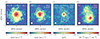 |
Fig. 1. Multi-wavelength imaging of BX610. (a) CO (4–3) integrated intensity map. The overlaid white contours correspond to the 3, 5, 7, 10, 20, 40, and 60σ levels. The filled circle at the bottom left corner indicates the ALMA-synthesized beam (θ = 0.18″ × 0.18″). (b) [CI] (1–0) integrated intensity map. The overlaid white contours, as in panels (c) and (d), represent the rest-frame optical emission observed by HST NICMOS/NIC2 F160W, corresponding to fractional flux levels relative to the maximum of 0.25, 0.5, and 0.75. (c) Rest-frame 630 μ m dust continuum emission. (d) Hα integrated intensity map. The filled circle at the bottom left corner indicates the SINFONI Hα point-spread function (θ = 0.24″ × 0.24″). |
2.2. Very Large Telescope
We include in our study VLT/SINFONI Adaptive Optics (AO)-assisted Hα observations from the SINS/zC-SINF survey (e.g., Förster Schreiber et al. 2009, 2014, 2018). We refer to Förster Schreiber et al. (2018) for a detailed description of the observation and further data reduction. In summary, the galaxy was observed in the K-band for an on-source time of 8.3 hr in LGS-SE AO mode. The achieved angular resolution was 0.24″ (a physical resolution of ≈2 kpc). To obtain the Hα flux map, we followed the line fitting described in Förster Schreiber et al. (2018). The right-most panel of Figure 1 shows the integrated Hα map. The emission peaks off-center, on a region of approximate kiloparsec size in the southwest, and is faint in the central region of BX610 as expected from dust obscuration.
2.3. Hubble Space Telescope
We include HST imaging of the rest-frame optical light based on a NICMOS/NIC2 observation using the F160W filter (approximately 480 nm at z = 2). A detailed description of the observations is provided by Förster Schreiber et al. (2011a) and Tacchella et al. (2015). We also use the stellar mass and visual extinction (AV) maps derived based on optical to NIR broadband spectral energy distributions as described in Tacchella et al. (2015).
3. Methods
3.1. Spectral stacking of the [CI] spectra
Since one of our main goals is to analyze radial trends in the molecular gas content and excitation properties in BX610, we need to maximize the detectability of the CO (4–3) and [CI] (1–0) emission lines across the entire galaxy. However, the signal-to-noise ratio (S/N) of the [CI] (1–0) emission line decreases more rapidly than that of the CO (4–3) line towards the outer regions. To enhance the detection of the [CI] (1–0) line, we employ a spectral stacking method as described by, for example, Schruba et al. (2011) and Villanueva et al. (2021).
The stacking procedure is as follows. First, we determine the central velocity of each spaxel in the CO (4–3) cube. Next, each [CI] (1–0) spaxel is shifted according to the CO (4–3) velocity field, to align the spectrum of each line of sight to zero velocity. The spectra are then averaged into radial bins defined by the galactocentric radius, with a bin width of 0.09″–half the beamsize of the data. This approach ensures that the radial bins do not oversample the radial profiles. To extract the line intensity, we fit a single-Gaussian profile to the averaged-stacked spectra. The uncertainties for each radial bin are calculated using the following equation
 (1)
(1)
where σ is the RMS of the emission-free portion of the stacked spectrum, N is the number of channels included in the mask, and Δv is the channel width in km s−1. To ensure reliable detection, we only consider [CI] (1–0) averaged-stacked spectra that exceed the 5σ level. Without stacking, the [CI] (1–0) line is initially detected up to 0.7 times one effective stellar radius. By stacking the data, on the other hand, we extend the reliable detection range beyond one stellar effective radius.
3.2. Molecular gas mass
Molecular gas masses are computed from the CO (4–3) and [CI] (1–0) line luminosities, which are defined by Solomon & Vanden Bout (2005) as
![Mathematical equation: $$ \begin{aligned} L\prime _{\rm line} \, \mathrm{\left[ K \, km \, s^{-1} \, pc^{2} \right]} = 3.25 \times 10^{7} S_{\rm line} \, {\Delta }{v} \, \nu _{\rm obs}^{-2} \, (1 + z)^{-3} \, D_{\rm L}^{2}, \end{aligned} $$](/articles/aa/full_html/2025/04/aa52652-24/aa52652-24-eq3.gif) (2)
(2)
where SlineΔv is the measured velocity-integrated line flux in Jy km s−1, νobs is the observed line frequency in GHz, z is the redshift of the source, and DL is the luminosity distance in Mpc.
The total cold molecular gas mass, Mmol, is then derived from the CO (4–3) line luminosity as
![Mathematical equation: $$ \begin{aligned} M_{\rm mol} \,\mathrm{\left[M_{\odot }\right]} = \alpha _{\rm CO} ~ R_{14} ~ L\prime _{\rm CO\,(4{-}3)}, \end{aligned} $$](/articles/aa/full_html/2025/04/aa52652-24/aa52652-24-eq4.gif) (3)
(3)
where αCO is the luminosity-to-molecular-gas-mass conversion factor, including a 36% contribution from helium, and R14 = L′CO (1 − 0)/L′CO (4 − 3) is the line luminosity ratio between the J = 4 → 3 and J = 1 → 0 transitions.
Several studies (e.g., Leroy et al. 2011; Genzel et al. 2012; Narayanan et al. 2012; Bolatto et al. 2013; Sandstrom et al. 2013) have shown that the αCO conversion factor can result in a wide range of values depending on the galaxy properties, including the density, temperature, and metallicity of the molecular clouds. While for local (U)LIRGs and starburst galaxies a value of αCO = 0.8 M⊙ (K km s−1 pc2)−1 is typically assumed (e.g., Downes & Solomon 1998), high redshift star-forming galaxies at the massive end of the main-sequence tend to have αCO values comparable to the standard Milky Way value of αMW = 4.36 M⊙ (K km s−1 pc2)−1 (Bolatto et al. 2013; Tacconi et al. 2020).
To derive the αCO value for BX610, we follow the calibration presented in Genzel et al. (2015) (also adopted in Tacconi et al. 2018), which combines the recipes given by Genzel et al. (2012) and Bolatto et al. (2013) through the geometric mean of both empirical functions. The αCO value based on the metallicity of the gas is given by,
![Mathematical equation: $$ \begin{aligned} \alpha _{\rm CO}&= \alpha _{\rm MW} \sqrt{10^{-1.27 \times \left(12 + \log \mathrm{(O/H)} - 8.67\right)}} \nonumber \\&\times \sqrt{0.67 \exp {\left[0.36 \times 10^{- \left(12 + \log \mathrm{(O/H)} - 8.67\right)}\right]}} \end{aligned} $$](/articles/aa/full_html/2025/04/aa52652-24/aa52652-24-eq5.gif) (4)
(4)
where 12 + log(O/H) is the metallicity on the Pettini & Pagel (2004) calibration scale, denoted as
![Mathematical equation: $$ \begin{aligned} \mathrm{12 + \log {(O/H)}}_{\rm PP04} = a - 0.087 \left[\log {(M_{\star }) - b}\right]^{2},\end{aligned} $$](/articles/aa/full_html/2025/04/aa52652-24/aa52652-24-eq6.gif) (5)
(5)
with a = 8.74 ± 0.06 and b = (10.4 ± 0.05)+(4.46 ± 0.3)×log(1 + z) − (1.78 ± 0.4)×[log(1 + z)]2 (Genzel et al. 2015, and references within). Based on the total stellar mass of BX610, we find a metallicity value of 12 + log(O/H) = 8.65 ± 0.07, which yields an αCO = 4.51 ± 0.60 M⊙ (K km s−1 pc2)−1.
The R14 line luminosity ratio converts the observed CO (4–3) line luminosity into the CO (1–0) line luminosity. Bolatto et al. (2015) conducted CO (1–0) observations on BX610 using the JVLA and detect a total line luminosity of L′CO (1 − 0) = (2.6 ± 0.2)×1010 K km s−1 pc2, which yields a line luminosity ratio of R14 = 1.1 ± 0.1. Under these assumptions and values, we find a molecular gas mass of Mmol = (1.2 ± 0.2)×1011 M⊙.
Alternatively, Mmol can be derived from the [CI]10 emission line (e.g., Weiß et al. 2005; Walter et al. 2011; Alaghband-Zadeh et al. 2013; Bothwell et al. 2017; Popping et al. 2017; Valentino et al. 2018), based on an estimated atomic mass of carbon, M[CI], and the assumption of a given neutral atomic carbon abundance X[CI]/X[H2]. The atomic carbon mass is estimated from the [CI] (1–0) line luminosity emission following the formula presented by Weiß et al. (2005)
![Mathematical equation: $$ \begin{aligned} M_{\rm [CI]} ~ \mathrm{\left[M_{\odot }\right]} = 5.706 \times 10^{-4} ~ Q(T_{\rm ex}) ~ \frac{\exp {(T_{1} / T_{\rm ex})}}{3} ~ L\prime _{\rm [CI]~(1{-}0)}, \end{aligned} $$](/articles/aa/full_html/2025/04/aa52652-24/aa52652-24-eq7.gif) (6)
(6)
where Q(Tex) = 1 + 3exp( − T1/Tex) + 5exp(T2/Tex) is the partition function, Tex is the excitation temperature, and T1 = 23.6 K and T2 = 62.5 K are the transition energy levels above ground state. Brisbin et al. (2019) recently measured Tex for BX610 based on the ![Mathematical equation: $ L{\prime}_\mathrm{[CI]~(2{-}1)} \big/ L{\prime}_\mathrm{[CI]~(1{-}0)} $](/articles/aa/full_html/2025/04/aa52652-24/aa52652-24-eq8.gif) line luminosity ratio and obtained a value of Tex = 31.8 ± 6.9 K, which is comparable to the typical dust temperature of Tdust ∼ 32 K found in massive (M⋆ ∼ 1011 − 1011.5 M⊙), main-sequence galaxies at z ∼ 2 (Magnelli et al. 2014; Genzel et al. 2015; Schreiber et al. 2018). We then estimate an atomic carbon mass value of M[CI] = (8.3 ± 0.9)×106 M⊙.
line luminosity ratio and obtained a value of Tex = 31.8 ± 6.9 K, which is comparable to the typical dust temperature of Tdust ∼ 32 K found in massive (M⋆ ∼ 1011 − 1011.5 M⊙), main-sequence galaxies at z ∼ 2 (Magnelli et al. 2014; Genzel et al. 2015; Schreiber et al. 2018). We then estimate an atomic carbon mass value of M[CI] = (8.3 ± 0.9)×106 M⊙.
To convert the carbon mass into a molecular gas mass, we need to assume a neutral atomic carbon abundance, X[CI]/X[H2] = M[CI]/6MH2. For instance, Valentino et al. (2018) compare the molecular hydrogen masses derived from CO and dust in a sample of main-sequence galaxies at z ∼ 1.2 and find abundances that range between 1 and 13 × 10−5, with a weighted mean of 1.5 × 10⁻⁵. Assuming this mean abundance, we measure a molecular hydrogen mass of MH2 = (9.5 ± 0.7)×1010 M⊙, which results in a molecular gas mass of Mmol = (1.3 ± 0.1)×1011 M⊙ (i.e., consistent with our CO-based measurement).
These CO- and [CI]-based molecular gas masses agree with the value reported previously by Bolatto et al. (2015), who estimated a molecular gas mass of Mmol = (1.1 ± 0.1)×1011 M⊙. However, these are a factor of ∼2 lower than the value found by Brisbin et al. (2019), who reported a molecular gas mass of Mmol = (2.1 ± 0.3)×1011 M⊙. This could be explained because Brisbin et al. (2019), as described in Section 2.1, measured a PdBI dust continuum that is a factor of ∼2 larger than the value reported in this work and in Lee et al. (2024).
3.3. Star formation rate
We measure the SFR from the Hα line using the calibration by Kennicutt (1998), modified for a Chabrier (2003) IMF, as follows
![Mathematical equation: $$ \begin{aligned} \mathrm{SFR_{\rm H{\alpha }} ~ \left[ M_{\odot } \,yr^{-1} \right]} = 4.7 \times 10^{-42} \,L_{\rm H{\alpha }, \,corr}, \end{aligned} $$](/articles/aa/full_html/2025/04/aa52652-24/aa52652-24-eq9.gif) (7)
(7)
where LHα, corr is the Hα luminosity in erg s−1 corrected for attenuation AHα, i.e., LHα, corr = LHα, obs × 100.4AHα. For the attenuation AHα, we use the extinction radial profiles measured by Tacchella et al. (2018) based on HST observations of the F438W (B) − F814W (I) index color. We assume a E(B − V)star/E(B − V)gas ratio of 0.44 (from Calzetti et al. 2000). Under these assumptions, we obtain a SFR of 140 M⊙ yr−1.
Additionally, in dusty environments such as the center of galaxies, the luminosity of young massive stars is frequently absorbed and then re-emitted in the IR, with an emission peak near 100 μm (e.g., Lutz et al. 2016). Therefore, the infrared emission can be a proxy for estimating the dust-obscured star formation. As can be seen from Figure 1, the molecular gas content as traced by the CO (4–3) and [CI] (1–0) transitions peaks at the center of the galaxy; however, the Hα line in this region is very faint. This is the result of strong dust obscuration in the center, where a correction based on the attenuation AHα measured from HST imaging is likely to underestimate the total star formation activity significantly. For this reason, in the central region of BX610, we use the ALMA dust continuum to measure the obscured star formation. First, we scale the ALMA Band 4 dust continuum flux to calculate the rest-frame 70 μm flux assuming a modified black-body (MBB, Casey 2012) with a spectral emissivity index β = 2 and a dust temperature Tdust = 30 K, as determined by Brisbin et al. (2019). The resulting flux is Scont, 70 μm = 13.2 mJy. Finally, we use the calibration by Calzetti et al. (2010) to measure the SFR based on the 70 μm continuum emission, which is given by
![Mathematical equation: $$ \begin{aligned} \mathrm{SFR_{70} ~ \left[ \mathrm{M_{\odot } \,yr}^{-1} \right]} = 5.9 \times 10^{-44} ~ L_{70}, \end{aligned} $$](/articles/aa/full_html/2025/04/aa52652-24/aa52652-24-eq10.gif) (8)
(8)
where L70 is the luminosity at 70 μm. Under these assumptions, we obtain a SFR of 114 M⊙ yr−1. Nevertheless, the dust continuum-based method has its own limitations. If we assume a dust temperature of Tdust = 40 K, the resulting SFR increases by a factor of 3.8. On the other hand, assuming a spectral emissivity index of β = 1.5, the SFR decreases by a factor of 3.0. Despite all these limitations, if we compare the obscured and unobscured SFR as traced by the dust continuum and uncorrected Hα emission, respectively, we measure an obscured fraction of star formation of 0.84. This is consistent with what has been observed in other massive star-forming galaxies at z ∼ 2 (e.g., Béthermin et al. 2015).
4. Results
4.1. Molecular gas excitation
With the development of wideband receivers that can simultaneously detect the CO (4–3) and [CI] (1–0) transitions in galaxies within certain redshift ranges (such as BX610 at z ≈ 2), the L′CO (4 − 3)/L′[CI] (1 − 0) line luminosity ratio has become an important tracer of both molecular gas chemistry and excitation (e.g., Alaghband-Zadeh et al. 2013; Bisbas et al. 2015; Bothwell et al. 2017; Valentino et al. 2018, 2020; Michiyama et al. 2021). However, considering that the excitation temperature of the [CI] (1–0) emission line is only about 1.5 times higher than that of the CO (2–1) emission line, and the critical density of the [CI] (1–0) line is approximately 4.4 times lower than that of the CO (1–0) transition (e.g., Carilli & Walter 2013), we expect molecular gas excitation to be the dominant effect traced by the L′CO (4 − 3)/L′[CI] (1 − 0) line luminosity ratio. To date, most studies have focused on global measurements of the L′CO (4 − 3)/L′[CI] (1 − 0) line luminosity ratio at high redshift. For example, in main-sequence star-forming galaxies at z ∼ 1, Valentino et al. (2020) find an average value of L′CO (4 − 3)/L′[CI] (1 − 0) = 2.13 ± 0.31. In the case of BX610, however, we now have the opportunity to explore excitation conditions on kiloparsec scales, extending out to one stellar effective radius thanks to our stacking technique. The left panel of Figure 2 presents the L′CO (4 − 3)/L′[CI] (1 − 0) line luminosity ratio map, normalized to the average value found in z ∼ 1 main-sequence galaxies (Valentino et al. 2020). We note that the molecular gas in the central regions of BX610 is significantly more excited than in the outskirts, with a line ratio nearly twice the typical global value found in z ∼ 1 main-sequence galaxies. Interestingly, the spiral arm extending southward, next to the giant star-forming clump detected in Hα emission, exhibits a line ratio comparable to that of z ∼ 1 main-sequence galaxies.
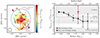 |
Fig. 2. Left: |
![Mathematical equation: $ L{\prime}_\mathrm{CO~(4{-}3)} \big/ L{\prime}_\mathrm{[CI]~(1{-}0)} $](/articles/aa/full_html/2025/04/aa52652-24/aa52652-24-eq11.gif)
![Mathematical equation: $ L{\prime}_\mathrm{CO~(4{-}3)} \big/L{\prime}_\mathrm{[CI]~(1{-}0)} $](/articles/aa/full_html/2025/04/aa52652-24/aa52652-24-eq12.gif)
The right panel of Figure 2 displays the radial profile of the L′CO (4 − 3)/L′[CI] (1 − 0) line luminosity ratio, with the radius normalized to the effective stellar radius in the bottom x-axis. At each radius, the profile is calculated by taking the ratio of the summed CO (4–3) line luminosities to the stacked [CI] (1–0) line luminosities. The emission from the star-forming clump is masked (based on the area marked by the red dashed aperture on the left panel) and shown separately (in red). In the central region ( ≲ 0.5 Reff, ⋆) of BX610, the line luminosity ratio is comparable to that found in local (U)LIRGs (e.g., Papadopoulos & Geach 2012). The high excitation levels observed in the center of BX610 could partly be influenced by the AGN hosted there. Studies have shown that the impact of central AGNs on CO excitation is typically confined to the innermost ∼0.5 kpc of galaxies (e.g., van der Werf et al. 2010; Pozzi et al. 2017; Mingozzi et al. 2018). Additionally, X-ray-dominated regions (XDRs) generated by the AGN can dominate the CO SLED, but this is only true for J > 5 transitions (e.g., Vallini et al. 2019), which are not part of this study.
Moving outwards, at around r ∼ 0.5 Reff, ⋆, the ratio decreases to levels similar to those observed in SMGs at z ∼ 2 − 4 (Valentino et al. 2020). Finally, in the range of r ∼ [0.75 − 1.25] Reff, ⋆, the line luminosity ratio is comparable to the typical values found in main-sequence star-forming galaxies at z ∼ 1 (Valentino et al. 2020). The star-forming clump, located at r ∼ 0.8 Reff, ⋆, exhibits a line luminosity ratio similar to that in the center of BX610, indicating elevated molecular gas excitation due to intense star formation. Notably, the global line luminosity ratio in BX610, L′CO (4 − 3)/L′[CI] (1 − 0) = 2.7 ± 0.7, is consistent with that observed in z ∼ 1 main-sequence galaxies (Valentino et al. 2020). This highlights the importance of spatially resolved observations in revealing the full range of molecular excitation conditions within galaxies, especially in regions of elevated star formation activity, such as central areas or extra-nuclear star-forming clumps.
4.2. Stellar, molecular, and star formation rate radial profiles
Figure 3 presents, from left to right, the radial profiles of stellar mass (Σ⋆), molecular gas mass (Σmol), and SFR (ΣSFR) surface densities in BX610. Similar to Figure 2, we mask the emission from the star-forming clump in all three panels and represent it as a single red point. The middle panel shows the molecular gas radial profile based on the CO emission. We choose the CO-based over the [CI]-based profile because CO emission extends farther across the disk, enabling the study of molecular gas surface density up to a radius of ∼1.5 Reff, ⋆. In the right panel, we present the radial profile of the SFR derived from extinction-corrected Hα emission (black squares) and from dust continuum emission (green squares). In the central region ( ≲ 0.5 Reff, ⋆), where ALMA detects dust continuum and Hα emission is faint, the dust continuum-based SFR is approximately five times higher than the extinction-corrected Hα-based SFR. This discrepancy is likely due to the optical extinction correction from Tacchella et al. (2018) being insufficient to fully account for the significant dust obscuration in the central region of BX610. However, it is important to note that the infrared-based SFR here is derived from dust continuum observations at a wavelength away from the peak of the infrared SED, introducing significant uncertainties. To obtain a more accurate measurement of the total SFR in the central region of BX610, ALMA dust continuum observations closer to the SED peak, such as those in Bands 8 or 9 (rest-frame ∼150 μm), are required.
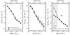 |
Fig. 3. Radial profiles of the stellar mass (left), molecular gas mass (middle), and SFR (right) surface densities of BX610, plotted with the same logarithmic dynamic range to facilitate comparison. Colors indicate the same as in Figure 2. In the right panel, green squares above the gray-shaded area are derived from the rest-frame 630 μm dust continuum emission, while black squares outside the area are derived from Hα corrected by dust attenuation profile of Tacchella et al. (2018). We also indicate for comparison the ΣSFR(Hα) data in the central region as black-filled squares, but with a dashed line. The vertical gray dotted line indicates the beam radius. We observe in the central region of the right panel that the SFRHα surface density is clearly underestimated in comparison with the SFRdust surface density. |
Additionally, we observe that both the star-forming clump and the disk have similar stellar mass surface densities values at r ∼ 0.8 Reff, ⋆. However, the clump shows slightly higher average values of Σmol and significantly higher values of ΣSFR at this galactocentric distance than the latter. This suggests that the elevated star formation activity in the clump is a result of the greater concentration of molecular gas compared to other regions of the disk. The similarity in Σ⋆ values between the disk and the clump at r ∼ 0.8 Reff, ⋆ suggests that the star formation activity is so recent that it has not yet led to a significant increase in the stellar mass of the clump region.
The left panel of Figure 4 shows the radial profile of the molecular gas fraction, μmol = Mmol/M⋆, which serves as an indicator of the gas available for star formation relative to the existing stellar content. We observe that in the central region ( ≲ 0.4 Reff, ⋆) of BX610, the molecular gas fraction is close to unity, and then it decreases to μmol ≈ 0.5 beyond one stellar effective radius. The global molecular gas fraction in BX610 is comparable to that measured in main-sequence star-forming galaxies at z ∼ 2 (μmol ≈ 0.75; Tacconi et al. 2020), but this is a result of averaging the high molecular gas fraction of μmol ≈ 1 measured at the central ∼2 kpc of BX610 with the μmol ≈ 0.5 in the outer parts. The star-forming clump in the southwest has an even higher molecular gas fraction than the central region (μmol ≈ 1.4), which is consistent with the elevated star formation activity traced by the Hα line. However, it is important to note that in the dusty central region of BX610, the SED-derived stellar mass may be underestimated.
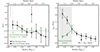 |
Fig. 4. Radial profiles of the molecular gas fraction (left) and the molecular gas depletion time (right) in BX610. Colors indicate the same as in Figure 3. The vertical gray dotted line indicates the beam radius. In the left panel, the green dashed line indicates the average molecular gas fraction measured by Tacconi et al. (2020) for main-sequence galaxies at z ∼ 2. |
The right panel of Figure 4 shows the molecular gas depletion time, tdep = Mmol/SFR, which represents the time required to deplete the molecular gas reservoirs at the current rate of star formation. In the inner ∼0.5 Reff, ⋆ (∼2 kpc) radius, the depletion timescale varies depending on whether we assume the extinction-corrected Hα-based (black squares) or the dust continuum-based SFR (green squares). Given the elevated concentration of molecular gas in the center and the strong dust continuum detected with ALMA, it is possible that the latter may be more representative of the total SFR in the nuclear region of BX610. If that is the case, then the depletion time decreases towards the center, reaching values of ≈450 Myr, which is consistent with depletion timescales measured in massive, star-forming galaxies at z ∼ 2 (e.g., Tacconi et al. 2020). The star-forming clump is the region with the lowest depletion time in BX610: the current level of star formation activity should exhaust the molecular gas in only ≈250 Myr. Moreover, the estimates derived on the timescales for gas to be depleted by SFR could be even shorter, given that ionized gas outflows are also observed at those locations (Förster Schreiber et al. 2014).
Placing these results in the broader context of galaxy evolution at cosmic noon, we infer that BX610 is likely in a phase where the rapid inflow of molecular gas into the central region, as reported by Genzel et al. (2023), has created a gas-rich nucleus (μmol ≈ 1), driving a high central star formation rate. This phase is commonly referred to as the wet compaction (Dekel & Burkert 2014; Zolotov et al. 2015; Tacchella et al. 2016). Following this phase, galaxies are expected to cease star formation in their centers before the outskirts, driven by a steep decline in the molecular gas fraction in the central kiloparsec region, consistent with findings in compact star-forming galaxies at z ∼ 2 in the process of inside-out quenching (e.g., Spilker et al. 2019).
4.3. Kennicutt–Schmidt Law
We explore the relationship between molecular gas surface density (Σmol) and star formation rate surface density (ΣSFR), as described by the Kennicutt–Schmidt law (Schmidt 1959; Kennicutt 1998). This relationship is key to understanding how efficiently cold gas is converted into stars across different environments (e.g., Genzel et al. 2010; Freundlich et al. 2013; Tacconi et al. 2013; Hodge et al. 2015; Chen et al. 2017; Sun et al. 2023; Villanueva et al. 2024). Figure 5 shows the resolved KS relation for BX610, with data points color-coded by radial distance and distinguished by shape according to specific regions within the galaxy. The figure is based on measurements from a grid of apertures across BX610, each with a diameter of 0.18″ (matching the beam size) and centers separated by 0.09″ to minimize flux loss from overlapping apertures. For the disk and clump regions, SFR values are derived from extinction-corrected Hα fluxes, while for the central regions, they are based on the ALMA dust continuum emission. Note that the use of Hα-based SFR for the center regions would result in a higher value of the molecular gas depletion time, as can be seen in the right panel of Figure 4.
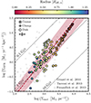 |
Fig. 5. Kennicutt–Schmidt diagram of BX610 for 0.18″ overlapped apertures of the center (crosses), the clump (stars), and the disk (circles). SFR values for disk and clump regions are derived from extinction-corrected Hα flux, while for central regions, they are based on dust continuum emission. The color bar indicates the distance to the center as a function of the stellar effective radius. A typical error bar is shown in the bottom right corner. The dotted diagonal lines correspond to constant gas depletion times of 0.1, 1, and 10 Gyr from top to bottom. The red dashed line correspond to the ordinary least-squares bisector fit for all data points. The gray data points from Genzel et al. (2010) and Tacconi et al. (2013) are indicated for comparison with whole galaxies, while the data points from Freundlich et al. (2013) are for spatially resolved main-sequence galaxies at z ∼ 1. |
Overall, the approximate kiloparsec-scale regions in BX610 align with the trend observed in spatially resolved studies of other massive, star-forming galaxies at z ∼ 1 − 2 (Tacconi et al. 2013; Freundlich et al. 2013; Genzel et al. 2013). Disk regions (circles) exhibit depletion timescales that scatter around ∼1 Gyr, with variations of about a factor of ∼2. As regions approach the center of BX610 (crosses), depletion times shorten, reaching close to ∼450 Myr. Notably, the extra-nuclear star-forming clump (stars) is the region in BX610 with the highest star formation efficiency, with a short depletion time of only ∼250 Myr. Applying an ordinary least-squares bisector fit to all the regions in BX610, we find that log(ΣSFR) = (1.27 ± 0.05)×log(Σmol) − (3.68 ± 0.17).
Similar to the case of the star-forming galaxy EGS13011166 at z ≈ 1.5 (Genzel et al. 2013), the fit will depend on the method by which the correction for dust obscuration is implemented. For EGS13011166, the slope ranges from 0.8 to 1.7, depending on the chosen extinction model. However, for the preferred mixed dust-gas model, Genzel et al. (2013) reported a super-linear slope of N = 1.14 ± 0.1, which is comparable, within uncertainties and assumptions, to the measured slope in BX610 of N = 1.27 ± 0.1.
5. Conclusions
We have conducted deep, high-angular-resolution (0.18″) ALMA Band 4 observations targeting the molecular gas traced by the CO (4–3) and [CI] (1–0) transitions in BX610, a massive main-sequence galaxy at z = 2.21. These observations, combined with VLT/SINFONI AO-assisted Hα emission line data (Förster Schreiber et al. 2018), have allowed us to characterize the molecular gas properties and star formation activity on approximate kiloparsec scales, spanning from the central regions to at least ∼1.5 (∼7 kpc) stellar effective radius in this typical star-forming galaxy at cosmic noon.
Our key findings are as follows:
-
By using the L′CO (4 − 3)/L′[CI] (1 − 0) line luminosity ratio as a tracer of molecular gas excitation in BX610, we find that the central region and the extra-nuclear, giant star-forming clump exhibit excitation levels comparable to those observed in nearby (U)LIRGs (Papadopoulos & Geach 2012). Beyond ∼0.5 Reff, ⋆, and on average across the disk, the molecular gas excitation conditions in BX610 resemble those typically found in normal star-forming galaxies at z ∼ 1 (e.g., Valentino et al. 2020).
-
The molecular gas fraction measured in the inner ∼2 kpc (∼0.5 Reff, ⋆) of BX610 and the giant star-forming clump in the southwest is high (μmol ≳ 1), resulting in intense star formation activity. Overall, the molecular gas fraction in the disk (μmol ≈ 0.5 − 0.7) is comparable to that globally measured in main-sequence, massive star-forming galaxies at z ≈ 2 (e.g., Tacconi et al. 2020). The molecular gas depletion times measured in the central region and in the giant star-forming clump are ∼450 Myr and ∼250 Myr, respectively.
-
The rapid transport of molecular gas to the central region of BX610 (Genzel et al. 2023), combined with the high central molecular gas fraction and short depletion timescale, suggests that BX610 may be undergoing a phase similar to the wet compaction scenario described in models by Dekel & Burkert (2014), Zolotov et al. (2015), and Tacchella et al. (2018). In this phase, the concentration of gas in the galaxy’s core drives intense star formation, which eventually leads to the inside-out quenching of star formation.
-
The approximate kiloparsec-scale regions in BX610 exhibit significant variations but generally align with the spatially resolved KS relation observed in other massive, star-forming galaxies at z ∼ 1 − 2 (e.g., Freundlich et al. 2013; Genzel et al. 2013; Tacconi et al. 2013). The overall slope and the depletion timescale measured in BX610 are N = 1.27 ± 0.05 and tdep ≈ 800 ± 400 Myr, respectively.
In summary, the deep, spatially resolved ALMA and VLT/SINFONI observations of BX610 provide one of the most detailed maps of molecular gas and star formation activity in a main-sequence, star-forming galaxy at cosmic noon. However, the absence of reliable measurements of obscured star formation in the central region limits our ability to interpret its physical conditions fully. Future ALMA observations at wavelengths closer to the SED peak (Band 8 or Band 9) or measurements of the Paschen-α line with JWST/MIRI are essential for addressing this issue and obtaining a more comprehensive understanding of the BX610 central region.
Acknowledgments
S.A.-N. and R.H.-C. thank the Max Planck Society for support under the Partner Group project “The Baryon Cycle in Galaxies” between the Max Planck for Extraterrestrial Physics and the Universidad de Concepción. S.A.-N. and R.H.-C. also gratefully acknowledge financial support from ANID BASAL projects FB210003. R.H.-C. also gratefully acknowledges financial support from ANID MILENIO – NCN2024_112. V. V. acknowledges support from the ALMA-ANID Postdoctoral Fellowship under the award ASTRO21-0062. N.M.F.S., J.C., G.T. acknowledge funding by the European Union through ERC Advanced Grant 101055023 “GALPHYS”, and H.Ü. acknowledges support from the European Union through ERC Starting Grant 101164796 “APEX.” Views and opinions expressed are, however, those of the author(s) only and do not necessarily reflect those of the European Union or the European Research Council. Neither the European Union nor the granting authority can be held responsible for them. This paper makes use of the following ALMA data: ADS/JAO.ALMA#2013.1.00059.S, ADS/JAO. ALMA#2017.1.01045.S and ADS/JAO.ALMA#2019.1.01362. ALMA is a partnership of ESO (representing its member states), NSF (USA) and NINS (Japan), together with NRC (Canada), NSTC and ASIAA (Taiwan), and KASI (Republic of Korea), in cooperation with the Republic of Chile. The Joint ALMA Observatory is operated by ESO, AUI/NRAO and NAOJ. This work is also based on observations collected at the Very Large Telescope of the European Southern Observatory under ESO programmes 183.A-0781(D) and 088.A-0202(A). This research made use of observations with the NASA/ESA Hubble Space Telescope obtained from the Space Telescope Science Institute, which is operated by the Association of Universities for Research in Astronomy, Inc., under NASA contract NAS 5-26555; these observations are associated with program GO 10924.
References
- Alaghband-Zadeh, S., Chapman, S. C., Swinbank, A. M., et al. 2013, MNRAS, 435, 1493 [Google Scholar]
- Aravena, M., Hodge, J. A., Wagg, J., et al. 2014, MNRAS, 442, 558 [Google Scholar]
- Béthermin, M., Daddi, E., Magdis, G., et al. 2015, A&A, 573, A113 [Google Scholar]
- Bisbas, T. G., Papadopoulos, P. P., & Viti, S. 2015, ApJ, 803, 37 [NASA ADS] [CrossRef] [Google Scholar]
- Bisbas, T. G., van Dishoeck, E. F., Papadopoulos, P. P., et al. 2017, ApJ, 839, 90 [Google Scholar]
- Bolatto, A. D., Wolfire, M., & Leroy, A. K. 2013, ARA&A, 51, 207 [CrossRef] [Google Scholar]
- Bolatto, A. D., Warren, S. R., Leroy, A. K., et al. 2015, ApJ, 809, 175 [NASA ADS] [CrossRef] [Google Scholar]
- Bolatto, A. D., Wong, T., Utomo, D., et al. 2017, ApJ, 846, 159 [Google Scholar]
- Bothwell, M. S., Aguirre, J. E., Aravena, M., et al. 2017, MNRAS, 466, 2825 [Google Scholar]
- Brisbin, D., Aravena, M., Daddi, E., et al. 2019, A&A, 628, A104 [EDP Sciences] [Google Scholar]
- Calzetti, D., Armus, L., Bohlin, R. C., et al. 2000, ApJ, 533, 682 [NASA ADS] [CrossRef] [Google Scholar]
- Calzetti, D., Wu, S. Y., Hong, S., et al. 2010, ApJ, 714, 1256 [NASA ADS] [CrossRef] [Google Scholar]
- Carilli, C. L., & Walter, F. 2013, ARA&A, 51, 105 [NASA ADS] [CrossRef] [Google Scholar]
- Casey, C. M. 2012, MNRAS, 425, 3094 [Google Scholar]
- Chabrier, G. 2003, PASP, 115, 763 [Google Scholar]
- Chen, C.-C., Hodge, J. A., Smail, I., et al. 2017, ApJ, 846, 108 [Google Scholar]
- Daddi, E., Bournaud, F., Walter, F., et al. 2010, ApJ, 713, 686 [NASA ADS] [CrossRef] [Google Scholar]
- Dekel, A., & Burkert, A. 2014, MNRAS, 438, 1870 [Google Scholar]
- Downes, D., & Solomon, P. M. 1998, ApJ, 507, 615 [NASA ADS] [CrossRef] [Google Scholar]
- Elmegreen, B. G., Elmegreen, D. M., Fernandez, M. X., & Lemonias, J. J. 2009, ApJ, 692, 12 [CrossRef] [Google Scholar]
- Erb, D. K., Steidel, C. C., Shapley, A. E., et al. 2006, ApJ, 646, 107 [NASA ADS] [CrossRef] [Google Scholar]
- Escala, A., & Larson, R. B. 2008, ApJ, 685, L31 [NASA ADS] [CrossRef] [Google Scholar]
- Förster Schreiber, N. M., Genzel, R., Bouché, N., et al. 2009, ApJ, 706, 1364 [Google Scholar]
- Förster Schreiber, N. M., Shapley, A. E., Erb, D. K., et al. 2011a, ApJ, 731, 65 [CrossRef] [Google Scholar]
- Förster Schreiber, N. M., Shapley, A. E., Genzel, R., et al. 2011b, ApJ, 739, 45 [Google Scholar]
- Förster Schreiber, N. M., Genzel, R., Newman, S. F., et al. 2014, ApJ, 787, 38 [Google Scholar]
- Förster Schreiber, N. M., Renzini, A., Mancini, C., et al. 2018, ApJS, 238, 21 [Google Scholar]
- Freundlich, J., Combes, F., Tacconi, L. J., et al. 2013, A&A, 553, A130 [NASA ADS] [CrossRef] [EDP Sciences] [Google Scholar]
- Genzel, R., Tacconi, L. J., Gracia-Carpio, J., et al. 2010, MNRAS, 407, 2091 [NASA ADS] [CrossRef] [Google Scholar]
- Genzel, R., Newman, S., Jones, T., et al. 2011, ApJ, 733, 101 [Google Scholar]
- Genzel, R., Tacconi, L. J., Combes, F., et al. 2012, ApJ, 746, 69 [Google Scholar]
- Genzel, R., Tacconi, L. J., Kurk, J., et al. 2013, ApJ, 773, 68 [NASA ADS] [CrossRef] [Google Scholar]
- Genzel, R., Tacconi, L. J., Lutz, D., et al. 2015, ApJ, 800, 20 [Google Scholar]
- Genzel, R., Jolly, J. B., Liu, D., et al. 2023, ApJ, 957, 48 [NASA ADS] [CrossRef] [Google Scholar]
- Glover, S. C. O., & Clark, P. C. 2016, MNRAS, 456, 3596 [Google Scholar]
- Glover, S. C. O., Clark, P. C., Micic, M., & Molina, F. 2015, MNRAS, 448, 1607 [NASA ADS] [CrossRef] [Google Scholar]
- Henríquez-Brocal, K., Herrera-Camus, R., Tacconi, L., et al. 2022, A&A, 657, L15 [NASA ADS] [CrossRef] [EDP Sciences] [Google Scholar]
- Hodge, J. A., Riechers, D., Decarli, R., et al. 2015, ApJ, 798, L18 [Google Scholar]
- Ikeda, M., Oka, T., Tatematsu, K., Sekimoto, Y., & Yamamoto, S. 2002, ApJS, 139, 467 [NASA ADS] [CrossRef] [Google Scholar]
- Ikeda, R., Tadaki, K.-I., Iono, D., et al. 2022, ApJ, 933, 11 [NASA ADS] [CrossRef] [Google Scholar]
- Kennicutt, R. C., Jr 1998, ARA&A, 36, 189 [NASA ADS] [CrossRef] [Google Scholar]
- Krumholz, M. R. 2014, Phys. Rep., 539, 49 [Google Scholar]
- Kulesa, C. A., Hungerford, A. L., Walker, C. K., Zhang, X., & Lane, A. P. 2005, ApJ, 625, 194 [NASA ADS] [CrossRef] [Google Scholar]
- Lee, M. M., Tanaka, I., Kawabe, R., et al. 2017, ApJ, 842, 55 [CrossRef] [Google Scholar]
- Lee, M. M., Tanaka, I., Iono, D., et al. 2021, ApJ, 909, 181 [NASA ADS] [CrossRef] [Google Scholar]
- Lee, M. M., Steidel, C. C., Brammer, G., et al. 2024, MNRAS, 527, 9529 [Google Scholar]
- Leroy, A. K., Bolatto, A., Gordon, K., et al. 2011, ApJ, 737, 12 [Google Scholar]
- Lutz, D., Berta, S., Contursi, A., et al. 2016, A&A, 591, A136 [NASA ADS] [CrossRef] [EDP Sciences] [Google Scholar]
- Madau, P., & Dickinson, M. 2014, ARA&A, 52, 415 [Google Scholar]
- Magnelli, B., Lutz, D., Saintonge, A., et al. 2014, A&A, 561, A86 [NASA ADS] [CrossRef] [EDP Sciences] [Google Scholar]
- McMullin, J. P., Waters, B., Schiebel, D., Young, W., & Golap, K. 2007, in Astronomical Data Analysis Software and Systems XVI, eds. R. A. Shaw, F. Hill, & D. J. Bell, ASP Conf. Ser., 376, 127 [Google Scholar]
- Michiyama, T., Saito, T., Tadaki, K.-I., et al. 2021, ApJS, 257, 28 [NASA ADS] [CrossRef] [Google Scholar]
- Mingozzi, M., Vallini, L., Pozzi, F., et al. 2018, MNRAS, 474, 3640 [NASA ADS] [CrossRef] [Google Scholar]
- Narayanan, D., & Krumholz, M. R. 2014, MNRAS, 442, 1411 [NASA ADS] [CrossRef] [Google Scholar]
- Narayanan, D., Krumholz, M. R., Ostriker, E. C., & Hernquist, L. 2012, MNRAS, 421, 3127 [NASA ADS] [CrossRef] [Google Scholar]
- Newman, S. F., Buschkamp, P., Genzel, R., et al. 2014, ApJ, 781, 21 [Google Scholar]
- Offner, S. S. R., Bisbas, T. G., Bell, T. A., & Viti, S. 2014, MNRAS, 440, L81 [NASA ADS] [CrossRef] [Google Scholar]
- Okada, Y., Güsten, R., Requena-Torres, M. A., et al. 2019, A&A, 621, A62 [NASA ADS] [CrossRef] [EDP Sciences] [Google Scholar]
- Papadopoulos, P. P., & Geach, J. E. 2012, ApJ, 757, 157 [NASA ADS] [CrossRef] [Google Scholar]
- Papadopoulos, P. P., Thi, W. F., & Viti, S. 2004, MNRAS, 351, 147 [NASA ADS] [CrossRef] [Google Scholar]
- Pettini, M., & Pagel, B. E. J. 2004, MNRAS, 348, L59 [NASA ADS] [CrossRef] [Google Scholar]
- Popping, G., Decarli, R., Man, A. W. S., et al. 2017, A&A, 602, A11 [NASA ADS] [CrossRef] [EDP Sciences] [Google Scholar]
- Pozzi, F., Vallini, L., Vignali, C., et al. 2017, MNRAS, 470, L64 [NASA ADS] [CrossRef] [Google Scholar]
- Requena-Torres, M. A., Israel, F. P., Okada, Y., et al. 2016, A&A, 589, A28 [NASA ADS] [CrossRef] [EDP Sciences] [Google Scholar]
- Rosenberg, M. J. F., van der Werf, P. P., Aalto, S., et al. 2015, ApJ, 801, 72 [Google Scholar]
- Sandstrom, K. M., Leroy, A. K., Walter, F., et al. 2013, ApJ, 777, 5 [Google Scholar]
- Schmidt, M. 1959, ApJ, 129, 243 [NASA ADS] [CrossRef] [Google Scholar]
- Schreiber, C., Elbaz, D., Pannella, M., et al. 2018, A&A, 609, A30 [NASA ADS] [CrossRef] [EDP Sciences] [Google Scholar]
- Schruba, A., Leroy, A. K., Walter, F., et al. 2011, AJ, 142, 37 [NASA ADS] [CrossRef] [Google Scholar]
- Solomon, P. M., & Vanden Bout, P. A. 2005, ARA&A, 43, 677 [NASA ADS] [CrossRef] [Google Scholar]
- Spilker, J. S., Aravena, M., Marrone, D. P., et al. 2015, ApJ, 811, 124 [NASA ADS] [CrossRef] [Google Scholar]
- Spilker, J. S., Bezanson, R., Weiner, B. J., Whitaker, K. E., & Williams, C. C. 2019, ApJ, 883, 81 [NASA ADS] [CrossRef] [Google Scholar]
- Sun, J., Leroy, A. K., Ostriker, E. C., et al. 2023, ApJ, 945, L19 [NASA ADS] [CrossRef] [Google Scholar]
- Tacchella, S., Lang, P., Carollo, C. M., et al. 2015, ApJ, 802, 101 [NASA ADS] [CrossRef] [Google Scholar]
- Tacchella, S., Dekel, A., Carollo, C. M., et al. 2016, MNRAS, 458, 242 [NASA ADS] [CrossRef] [Google Scholar]
- Tacchella, S., Carollo, C. M., Förster Schreiber, N. M., et al. 2018, ApJ, 859, 56 [Google Scholar]
- Tacconi, L. J., Neri, R., Genzel, R., et al. 2013, ApJ, 768, 74 [NASA ADS] [CrossRef] [Google Scholar]
- Tacconi, L. J., Genzel, R., Saintonge, A., et al. 2018, ApJ, 853, 179 [Google Scholar]
- Tacconi, L. J., Genzel, R., & Sternberg, A. 2020, ARA&A, 58, 157 [NASA ADS] [CrossRef] [Google Scholar]
- Teague, R., & Foreman-Mackey, D. 2018, Research Notes of the American Astronomical Society, 2, 173 [Google Scholar]
- Valentino, F., Magdis, G. E., Daddi, E., et al. 2018, ApJ, 869, 27 [Google Scholar]
- Valentino, F., Magdis, G. E., Daddi, E., et al. 2020, ApJ, 890, 24 [Google Scholar]
- Vallini, L., Tielens, A. G. G. M., Pallottini, A., et al. 2019, MNRAS, 490, 4502 [CrossRef] [Google Scholar]
- van der Werf, P. P., Isaak, K. G., Meijerink, R., et al. 2010, A&A, 518, L42 [NASA ADS] [CrossRef] [EDP Sciences] [Google Scholar]
- Villanueva, V., Bolatto, A., Vogel, S., et al. 2021, ApJ, 923, 60 [Google Scholar]
- Villanueva, V., Bolatto, A. D., Vogel, S. N., et al. 2024, ApJ, 962, 88 [NASA ADS] [CrossRef] [Google Scholar]
- Walter, F., Weiß, A., Downes, D., Decarli, R., & Henkel, C. 2011, ApJ, 730, 18 [Google Scholar]
- Walter, F., Carilli, C., Neeleman, M., et al. 2020, ApJ, 902, 111 [Google Scholar]
- Weiß, A., Downes, D., Henkel, C., & Walter, F. 2005, A&A, 429, L25 [NASA ADS] [CrossRef] [EDP Sciences] [Google Scholar]
- Zolotov, A., Dekel, A., Mandelker, N., et al. 2015, MNRAS, 450, 2327 [Google Scholar]
All Tables
All Figures
|
Fig. 1. Multi-wavelength imaging of BX610. (a) CO (4–3) integrated intensity map. The overlaid white contours correspond to the 3, 5, 7, 10, 20, 40, and 60σ levels. The filled circle at the bottom left corner indicates the ALMA-synthesized beam (θ = 0.18″ × 0.18″). (b) [CI] (1–0) integrated intensity map. The overlaid white contours, as in panels (c) and (d), represent the rest-frame optical emission observed by HST NICMOS/NIC2 F160W, corresponding to fractional flux levels relative to the maximum of 0.25, 0.5, and 0.75. (c) Rest-frame 630 μ m dust continuum emission. (d) Hα integrated intensity map. The filled circle at the bottom left corner indicates the SINFONI Hα point-spread function (θ = 0.24″ × 0.24″). |
| In the text | |
|
Fig. 2. Left: |
| In the text | |
|
Fig. 3. Radial profiles of the stellar mass (left), molecular gas mass (middle), and SFR (right) surface densities of BX610, plotted with the same logarithmic dynamic range to facilitate comparison. Colors indicate the same as in Figure 2. In the right panel, green squares above the gray-shaded area are derived from the rest-frame 630 μm dust continuum emission, while black squares outside the area are derived from Hα corrected by dust attenuation profile of Tacchella et al. (2018). We also indicate for comparison the ΣSFR(Hα) data in the central region as black-filled squares, but with a dashed line. The vertical gray dotted line indicates the beam radius. We observe in the central region of the right panel that the SFRHα surface density is clearly underestimated in comparison with the SFRdust surface density. |
| In the text | |
|
Fig. 4. Radial profiles of the molecular gas fraction (left) and the molecular gas depletion time (right) in BX610. Colors indicate the same as in Figure 3. The vertical gray dotted line indicates the beam radius. In the left panel, the green dashed line indicates the average molecular gas fraction measured by Tacconi et al. (2020) for main-sequence galaxies at z ∼ 2. |
| In the text | |
|
Fig. 5. Kennicutt–Schmidt diagram of BX610 for 0.18″ overlapped apertures of the center (crosses), the clump (stars), and the disk (circles). SFR values for disk and clump regions are derived from extinction-corrected Hα flux, while for central regions, they are based on dust continuum emission. The color bar indicates the distance to the center as a function of the stellar effective radius. A typical error bar is shown in the bottom right corner. The dotted diagonal lines correspond to constant gas depletion times of 0.1, 1, and 10 Gyr from top to bottom. The red dashed line correspond to the ordinary least-squares bisector fit for all data points. The gray data points from Genzel et al. (2010) and Tacconi et al. (2013) are indicated for comparison with whole galaxies, while the data points from Freundlich et al. (2013) are for spatially resolved main-sequence galaxies at z ∼ 1. |
| In the text | |
Current usage metrics show cumulative count of Article Views (full-text article views including HTML views, PDF and ePub downloads, according to the available data) and Abstracts Views on Vision4Press platform.
Data correspond to usage on the plateform after 2015. The current usage metrics is available 48-96 hours after online publication and is updated daily on week days.
Initial download of the metrics may take a while.