| Issue |
A&A
Volume 696, April 2025
|
|
|---|---|---|
| Article Number | A174 | |
| Number of page(s) | 21 | |
| Section | Planets, planetary systems, and small bodies | |
| DOI | https://doi.org/10.1051/0004-6361/202450128 | |
| Published online | 25 April 2025 | |
Can metal-rich worlds form by giant impacts?
1 Department of Earth, Atmospheric and Planetary Sciences, Massachusetts Institute of Technology, 77 Massachusetts Ave Bldg 54, Cambridge, MA 02139, USA
2 Lunar and Planetary Laboratory, The University of Arizona, 1629 E University Blvd, Tucson, AZ 85721, USA
3 Planetary Science Institute, Tucson, 1700 E Fort Lowell Rd STE 106, Tucson, AZ 85719, USA
4 Universitäts-Sternwarte, Ludwig-Maximilians-Universität München, Scheinerstraße 1, 81679 München, Germany
★ Corresponding author; This email address is being protected from spambots. You need JavaScript enabled to view it.
Received:
25
March
2024
Accepted:
10
March
2025
Abstract
Context. Astronomical observations revealed the existence of exoplanets whose densities are far higher than what is expected from cosmochemistry. This high-density planetary population may account for 9% of terrestrial planets, suggesting the existence of processes that form planets with compositions dramatically different from their starting materials.
Aims. A commonly invoked theory is that these high-density exoplanets are the metallic cores of super–Earth-sized planets whose rocky mantle was stripped by giant impacts. Here we aim to test this hypothesis.
Methods. To maximize the likelihood that metal-rich giant-impact remnants form, we model the late orbital instability of tightly packed super-Earths orbiting a host star at small stellocentric distances (“compact systems”). We combine orbital dynamics, impact physics, and machine learning to explore the stability and collisional evolution of 100 observed compact systems. In each unstable compact system, we assume that the super-Earths undergo giant impacts and explore 1000 possible collision scenarios. We repeat the simulations with different initial conditions, such as the initial masses and composition of the super-Earths.
Results. We find that giant impacts are capable of stripping the mantles of super-Earths and form metal-rich worlds as massive and large as the observed high-density exoplanets. However, we also find that, in most of the explored scenarios, mantle-stripping giant impacts between super-Earths are unlikely to occur at rates sufficient to explain the size and currently estimated abundance of the observed high-density exoplanets. We explain this as the interplay of three factors: the size of the super-Earths being in most cases smaller than 2 Earth radii; the efficiency of mantle stripping decreasing with increasing planetary size; and the likelihood of compact system instability decreasing with increasing average sizes of the planets in the compact system.
Conclusions. We conclude that most of the observed high-density exoplanets are unlikely to be metal-rich giant-impact remnants.
Key words: methods: numerical / planets and satellites: composition / planets and satellites: dynamical evolution and stability / planets and satellites: formation / planets and satellites: physical evolution / planets and satellites: terrestrial planets
© The Authors 2025
 Open Access article, published by EDP Sciences, under the terms of the Creative Commons Attribution License (https://creativecommons.org/licenses/by/4.0), which permits unrestricted use, distribution, and reproduction in any medium, provided the original work is properly cited.
This article is published in open access under the Subscribe to Open model. This email address is being protected from spambots. You need JavaScript enabled to view it. to support open access publication.
1 Introduction
Planets and their host stars accrete materials from the same reservoirs (e.g., Adibekyan et al. 2021). Planet formation models therefore commonly assume that the abundance of refractory planet-forming elements in protoplanetary disks (e.g., Fe, Mg, Si) matches that inferred from spectroscopic observations of planet-hosting stars. However, the theory that planets and host stars are always compositionally linked is challenged by the existence of high-density exoplanets, here defined as cosmochemical outliers with bulk density higher than the 99.7th percentile of values expected from the host-star abundances of planet-forming elements (Unterborn et al. 2023, Section 2.1). Exoplanetary survey data suggest that these high-density exoplanets may account for ~9% of all terrestrial planets (Section 2.1.2). How such a large population of high-density exoplanets formed is unknown, but two main theories exist.
High-density exoplanets could be the fossil-compressed silicate-iron cores of giant planets that lost their volatile-rich envelopes through tidal stripping during close encounters with their host stars or as the result of photoevaporation driven by extreme ultraviolet stellar radiation (Faber et al. 2005; Mocquet et al. 2014). In this case, the observed high-density exoplanets are predicted to remain high-density up to 1 billion year (Gyr) as the core decompresses following loss of the envelope (Mocquet et al. 2014). However, a recent study suggest that naked cores are unlikely to retain a fossil compression state because a large fraction, if not all, of them was molten during the planet’s early evolution and can rapidly rebound due to low viscosity (Lin et al. 2025). Alternatively, high-density exoplanets could be metal-rich worlds with a high (≥50–60 wt.%) iron content compared with Earth, whose metal content (~30 wt.%, or 16 vol.%) is close to that of CI carbonaceous chondrites and the Sun’s refractory element fraction (Palme & O’Neill 2003). Examples of metal-rich worlds in the Solar System are the planet Mercury and asteroid (16) Psyche, whose metal contents are ~70 wt.% and ~30–60 vol%, respectively (Ebel & Stewart 2018; Elkins-Tanton et al. 2022).
In turn, metal-rich worlds could form in at least two ways. First, metal-rich worlds may form via preferential accretion of metal-rich materials near the condensation/sublimation line of refractory elements in the innermost part of protoplanetary disks (e.g., Aguichine et al. 2020; Johansen & Dorn 2022). Second, differentiated planets with a rocky mantle and a metallic core and with a metal-to-silicate ratio comparable to their host stars’ may evolve into metal-rich worlds by losing their mantles in giant impacts (e.g., Marcus et al. 2009; Asphaug & Reufer 2014; Reinhardt et al. 2022). Recent advances in analytical impact theory and modeling have enabled tests of the latter hypothesis. For example, previous studies have shown that Mercury analogs can form as a result of collisional grinding of terrestrial embryos in the early Solar System (e.g., Cambioni et al. 2021), when the gravitational interactions between the growing planets overwhelm the damping effects of the dissipating nebular gas and smaller planetesimals, leading to crossing orbits (Kenyon & Bromley 2006; O’ Brien et al. 2006).
Analogously to what has been proposed for planet Mercury, the observed high-density exoplanets could be the metallic cores of super-Earths that lost their mantles in giant impacts (Marcus et al. 2009; Reinhardt et al. 2022). However, because the gravitational binding energy of a planet increases with planetary size to the fifth power, stripping a super-Earth’s mantle requires collisions with at least one order of magnitude higher specific impact energy than those needed to remove the mantle of proto-Mercury (Marcus et al. 2009; Reinhardt et al. 2022; Gabriel & Cambioni 2023). It is unclear whether these impact energies may be achieved during planet formation and evolution. For a given colliding pair, the impact energy is defined by the collision velocity,
 (1)
where vesc is the mutual escape velocity defined as
(1)
where vesc is the mutual escape velocity defined as
 (2)
where G is the gravitational constant, M is the planetary mass, R is the planetary radius, and the subscripts “T “ and “P” indicate the target and projectile of the collision, here defined as the bodies with the largest and smallest binding energies, respectively.
(2)
where G is the gravitational constant, M is the planetary mass, R is the planetary radius, and the subscripts “T “ and “P” indicate the target and projectile of the collision, here defined as the bodies with the largest and smallest binding energies, respectively.
The variable v∞ is the pre-encounter relative velocity of the colliding bodies. If vcoll ~ vesc, planets are expected to merge with little to no debris production. vcoll ≫ vesc is therefore required to strip planets of their mantles.
During the growth of terrestrial planets, giant impacts between planetary embryos tend to occur at vcoll ~ vesc (Figure 1a). Under Solar System conditions, these events can preferentially erode mantle materials over core materials, forming Earth analogs with core-mass fractions of at most 0.4 (e.g., Chambers 2013; Cambioni et al. 2021; Allibert et al. 2025). However, this metal enrichment is significantly lower than that necessary to match the densities of the observed high-density exoplanets (Figure 2). Similar results are obtained for exoplanetary systems featuring giant impacts between super-Earths-sized planets (e.g., Scora et al. 2020; Poon et al. 2020; Esteves et al. 2022; Goldberg & Batygin 2022). In formation studies that maximize the likelihood of mantle stripping by assuming that planetary embryos are small and on eccentric orbits (that is, high v∞ and low vesc; e.g., Scora et al. 2022), the resulting metal-rich planets are smaller than GJ 367 b, which we identify as the smallest observed high-density exoplanet (Table 1; Section 2.1). Overall, planet formation models predict that giant impacts between growing super-Earths generally occur at impact energies lower than those necessary for mantle stripping.
After formation ceases, super-Earths can remain on short-period orbits that are tightly packed around their host stars; these configurations are commonly referred to as compact systems (Weiss et al. 2023, Figure 1b). Planets in compact systems can experience eccentricity growth due to the overlapping of mean-motion resonances and secular resonances (Volk & Gladman 2015; Pu & Wu 2015; Tamayo et al. 2020; Volk & Malhotra 2020, 2024). This can eventually result in orbital instability (Figure 1c) and a phase of crossing orbits and giant impacts that occurs significantly after the initial era of planet formation [>10 million years (Myr), potentially up to Gyr (Volk & Gladman 2015; Tamayo et al. 2020)]. Because v∞ increases with decreasing stellocentric distances and increasing mutual eccentricities (Gabriel & Cambioni 2023), giant impacts during this late period of orbital instability are likely to be more energetic (vcoll ≫ vesc), and thus more likely to strip the super-Earths’ mantles, than impacts occurring in previous planet formation eras.
Motivated by this, here we combine exoplanetary observations, N-body simulations, smoothed particle hydrodynamic (SPH) simulations of giant impacts, and machine learning to test the hypothesis that giant impacts between super-Earths with a bulk composition with the average local galactic abundance of iron and rock-forming elements may form metal-rich worlds akin to the observed high-density exoplanets (Figure 1d). In particular, we set an upper limit on the rate with which orbital instabilities in compact systems can produce metal-rich giant-impact remnants.
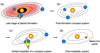 |
Fig. 1 Formation theory for the observed high-density exoplanets. (a) Super-Earths are predicted to complete their formation through giant impacts whose energies are too low to strip their rocky mantles and form metal-rich planets (Scora et al. 2020, 2022; Poon et al. 2020; Esteves et al. 2022; Goldberg & Batygin 2022). (b) After their formation ceases, super-Earths can remain on closely spaced orbits typical of observed compact systems (Weiss et al. 2023) and can experience instabilities over timescales comparable to the main-sequence lifetime of their host stars (Volk & Gladman 2015; Pu & Wu 2015; Tamayo et al. 2020; Volk & Malhotra 2020). (c) If a compact system becomes unstable, super-Earths can experience a second stage of giant impacts that are more energetic than those that occurred during their formation (Volk & Gladman 2015). These late giant impacts may erode the silicate mantles of the super-Earths to form metal-rich, high-density planets. (d) The post-instability planetary systems may have a metal-rich world with density akin to the measured densities of observed high-density exoplanets (Table 1). Colors indicate different planetary compositions: orange is metal-rich, blue indicates planets with a terrestrial composition (that is, differentiated in an iron core and a rocky mantle with core-mass fraction ∼30 wt.%). |
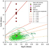 |
Fig. 2 Abundance of iron and rock-forming elements in the galactic neighborhood, selected planets, and meteorites. The green data points are the iron-to-silicon (Fe/Si) molar ratio versus magnesium-to-silicon (Mg/Si) molar ratio of stars with planets in the Hypatia catalog by Hinkel et al. (2014), along with the 68% (1σ), 95% (2σ) and 99.7% (3σ) isocontours, and the (Fe/Si, Mg/Si) of the CI carbonaceous chondrites, Earth, Mercury, and some of the high-density exoplanets in Table 1. The Fe/Si and Mg/Si values of the high-density exoplanets and Mercury are unknown. Here we assume that these planets have a Mg/Si equal to that of CI chondrites (the high-density nature of these planets does not change if other Mg/Si values are assumed). We then derive the bulk Fe/Si of planets from estimates of their core-mass fraction, Z, based on the measured masses and radii. We convert Z into Fe/Mg versus Si/Mg using Equation (13) from Unterborn et al. (2023), assuming that all the iron of the planet is in the core and that the mantle is composed of SiO2 and MgO. This plot is similar to Figure 7 from Unterborn et al. (2023), but here we plot only stars whose abundances [Fe/H], [Mg/H], and [Si/H] are known with uncertainties smaller than 30% and convert these values to molar ratios using the method by Hinkel et al. (2022). |
2 Data and methods
2.1 High-density exoplanets
We assume that the high densities of high-density exoplanets are diagnostic of an anomalously high abundance of metals and do not indicate that these planets are fossil-compressed iron-rock-ice cores of gas giants (we revisit this alternative proposal in Section 4). Based on this assumption, we define a high-density exoplanet as a planet that has bulk density, ρ, higher than ρHD, which is the density corresponding to the 99.7th percentile of densities predicted for planets based on the abundance of iron and rock-forming elements measured in stars. Following Unterborn et al. (2023), we define ρHD (in cgs units) as
 (3)
(3)
where  indicates the density of a planet of the same radius, R (in units of Earth radii, R⊕) and a bulk composition with the average local galactic abundance of iron and rock-forming elements (Mg/Si ~ 1.11 and Fe/Si ~ 0.89 molar ratios). The latter is close to that of CI carbonaceous chondrites (Figure 2). Planetary bodies with a bulk composition like CI chondrites are expected to differentiate into a rocky mantle and an iron core with a core-mass fraction, Z, of about 0.33, which is close to Earth’s (Palme & O’Neill 2003). Differentiated iron-rock planets with Z ~ 0.2 and Z ~ 0.4 would instead have an iron content one standard deviation (σ) below and above the CI chondritic value, respectively (dashed lines tangent to the 68% isocontour in Figure 2).
Equation (3) is valid for planets with R ≲ 2R⊕ and yields the 99.7th percentile of densities for planets in the “nominally rocky planet zone,” that is, the region of the mass-radius parameter space where planetary abundances of iron and rock-forming elements are within the 99.7% equal-tailed interval of the distribution for planet-hosting stars. Using the stellar compositional data from the Hypatia Catalog by Hinkel et al. (2014) (Figure 2), Unterborn et al. (2023) derived the nominally rocky planet zone by solving five coupled differential equations: the mass within a sphere; the temperature-dependent equation of state for the constituent minerals from Connolly (2009) and Anderson & Ahrens (1994) for the mantle and core, respectively; the equation of hydrostatic equilibrium; the adiabatic temperature profile; and Gauss’ law of gravity in one-dimension. For more details, we refer the reader to Unterborn et al. (2023).
Known high-density exoplanets.
2.1.1 Identification of high-density exoplanets
To identify high-density exoplanets in the NASA Exoplanet catalog as of February 23, 2024, we looked for planets that orbit a single star and have radii and masses known with uncertainties smaller than 30%, that is, σR/R < 0.3 and σM/M < 0.3 (as in previous studies, Adibekyan et al. 2021; Unterborn et al. 2023). Next, we sampled 105 mass-radius pairs within the uncertainty ellipses of these planets, computed the corresponding ρ assuming a spherical body, and declared the planet “high-density” if the fraction pHD of mass-radius pairs for which ρ > ρHD is larger than or equal to 68% (that is, these planets are high-density at least at the 1-σ confidence level). This search yielded a preliminary catalog of 13 high-density exoplanets.
Importantly, our preliminary catalog of high-density exo-planets includes three planets whose masses were estimated from analysis of transit-timing variations (TTVs): Kepler-245 c, Kepler-105 c, and Kepler-80 d. Previous studies have shown that analysis of TTVs for systems near first-order mean–motion resonances can overestimate the planetary mass when the estimated eccentricities are high (e.g., see Equations (6) and (7) in Hadden & Lithwick 2014). Kepler-245 c and Kepler-105 c were respectively flagged as high-eccentricity and low-eccentricity by Hadden & Lithwick (2014). The mass of Kepler-80 d was derived by restricting the TTV fits to the low-eccentricity regime by MacDonald et al. (2016), who ran robustness tests to show that for the Kepler-80 system the mass–eccentricity degeneracy does not preclude reliable mass estimates. Following this, we decided to remove only Kepler-245 c from the aforementioned preliminary list. This shortened the list to 12 high-density exo-planets, whose M, R, ρ, and pHD are in Table 1.
The bulk densities of the high-density exoplanets in Table 1 range from 1.4 to 2.7 times those of similar-sized planets with an Earth-like composition. Under the assumption that these densities are proxies for high metal content, high-density exoplanets are differentiated in a large (⪺50 wt.%) iron-rich core overlaid by a thin mantle made of rock-forming elements (Figure 2). This interior structure resembles that of planet Mercury (Ebel & Stewart 2018), whose iron content is also above the 99.7th percentile of values expected from stellar cosmochemistry (Figure 2) with Z ~ 70% as measured by the NASA MESSENGER mission (e.g., Nittler et al. 2018). This has motivated the term “super-Mercuries” commonly used in the literature to refer to high-density exoplanets.
2.1.2 Occurrence rate of high-density exoplanets
The high (⪺50 wt.%) iron content expected for high-density exo-planets makes them the iron-rich end-members of the terrestrial planets, a family of astronomical bodies whose interior structure is thought to consist of an iron core overlaid by a rocky mantle, with a generally small (but hard to quantify) amount of lower-density compounds (Figure 2). We aim to compute the occurrence rate of the high-density exoplanets among the terrestrial planets, ηHD, and compare this metric to that from our simulations to test the hypothesis that mantle-stripping giant impacts between terrestrial planets occur at rates sufficient to explain the currently estimated abundance of the high-density exoplanets.
Estimating ηHD requires identifying those planets in the catalog that are terrestrial based on their measured masses and radii. This is challenging because there exists a significant degeneracy of compositions that can match a planet’s measured mass and radius even when uncertainties are not taken into account. This prevents the amount of iron, rock, and lower-density compounds in exoplanets from being quantified precisely. Furthermore, how the relative abundances of iron, rock, and lower-density compounds would affect the measured radii and masses depends on their chemical phase, miscibility, and partition coefficients. Surface water could be present in the form of liquid or ice, or even be dissolved in the interior (Luo et al. 2024). Elements that are typically considered to be atmophiles (e.g., H, C) can partition into the core of terrestrial planets at the few wt.% level, as it has been inferred for Earth and Mars (e.g., McDonough 2003; Irving et al. 2023).
Nevertheless, exoplanetary studies have long predicted that there should be a radius gap between “volatile-rich” planets and terrestrial planets, owing to atmospheric evaporation driven by the high-energy photons from stars, which is more efficient on smaller planets at a given stellocentric distance (see Owen 2019, for a review). Consistently, exoplanetary observations have revealed a scarcity of planets with 1.5 R⊕ ≲ R ≲ 2 R⊕, known as the radius valley (e.g., Zhu & Dong 2021, for a review; whether the radius valley is indeed due to photoevaporation or instead core-powered mass loss is still debated). Furthermore, the mass-radius distributions of exoplanets was found to change slope at the radius valley, suggesting a transition from an interior structure dominated by iron/rock to one dominated by volatiles (e.g., Otegi et al. 2020, and references therein). We therefore leveraged the discovery of the radius valley to compute the value of ηHD based on data from NASA Exoplanet Archive according to two criteria.
First, we assumed that the upper edge of the radius valley (that is, R ≈ 2 R⊕) is the maximum possible radius for a terrestrial planet. Based on this criterion, we identified a sample of 85 terrestrial planets which includes the 12 high-density exoplanets identified in Section 2.1, corresponding to ηHD = 12/85 = 14%. Second, we defined a terrestrial planet as having M and R within 1σ of those predicted by the mass-radius relationship for “rocky planets” by Otegi et al. (2020). We used their mass-radius relationship to compute the radius given the measured mass, obtaining a sample of 84 terrestrial planets, to which we added the 12 high-density exoplanets whose radii are too small to be captured by the mass-radius relationship by Otegi et al. (2020) for a given mass. This yields ηHD = 12/(84 + 12) = 12.5%. The average ηHD calculated from the criteria above is ~13%. The list and properties of the terrestrial planets from the different scenarios are in the Supplementary Dataset S1.
A further challenge in estimating ηHD is that most masses of exoplanets in the catalog are measured through the radial-velocity (RV) method, which is known to provide better constraints on the mass of more massive exoplanets than for less massive exoplanets of the same size, assuming all other properties (e.g., orbit period) are equal (e.g., Steffen 2016). This can lead to an overestimation of ηHD. To account for the RV bias, we corrected ηHD as described in the Appendix A (see also Figure A.1), lowering it from 13% to 9%. Note that the preferential detection of closer-in, larger exoplanets also affects the completeness of the terrestrial planet database. We address this bias in Section 2.4.1.
We note that a previous study reported a higher ηHD = 23% based on the detection of five high-density exoplanets among a group of 22 terrestrial planets (Adibekyan et al. 2021). However, their sample included K2-38 b, for which we estimated a pHD of 55%, lower than the 1σ threshold adopted here, and K2-106 b, whose nature as a high-density exoplanet has been recently revisited (Rodríguez Martínez et al. 2023). If we reject both K2-38 b and K2-106 b from the sample by Adibekyan et al. (2021) and apply the RV correction, their ηHD lowers to 9%, consistent with our estimate.
2.2 Model of orbital instability of compact systems
Super–Earth-sized planets are expected to conclude their growth through a phase of giant impacts (Section 1; Gabriel & Cambioni 2023, for a review). However, these events are not sufficiently energetic to strip their mantles and form high-density exoplanets akin to those observed (Scora et al. 2020; Poon et al. 2020; Esteves et al. 2022; Goldberg & Batygin 2022). Super-Earths can later assemble in compact systems that undergo instability >10 Myr, potentially up to Gyr after formation ceases, leading to a second phase of giant impacts (Volk & Gladman 2015; Pu & Wu 2015; Tamayo et al. 2020; Volk & Malhotra 2020, 2024). Here we investigate whether these later giant impacts can form metal-rich worlds as large as those observed.
2.2.1 N-body simulations
The orbital stability and collisional evolution of planetary systems is traditionally studied using N-body simulations (e.g., Volk & Gladman 2015; Tamayo et al. 2020). These simulations evolve the orbits of planets under their mutual gravitational interaction and model close encounters and collisions. To showcase this, we simulated the orbital evolution of the four super-Earths in the compact system Kepler-402 using REBOUNDx including post-Newtonian general relativity orbital corrections using the gr-package. We initialized the eccentricity and mean longitudes of these planets with values that are predicted to lead to instability according to the Stability of Planetary Orbital Configurations Klassifier, SPOCK (Tamayo et al. 2020). Initial eccentricities were kept below 0.1, consistent with constraints from transit timing variations (Hadden & Lithwick 2017). Any collision between the planets was modeled using the collision model described in Section 2.2.3.
The result for Kepler-402 is in Figure 3, which plots the evolution of the semimajor axis, a [measured in astronomical units (au)] as a function of time, t. The orbital instability features the two innermost planets and the two outermost planets that merge pairwise to form two larger planets. No planet becomes metal-rich in this simulation [that is, no planet acquires a bulk density higher than ρHD, defined in Equation (3)], but a different outcome is possible for different initial eccentricities and mean longitudes.
However, using N-body simulations to comprehensively explore the parameter space of initial orbits across multiple compact systems and effectively couple N-body and SPH simulations is currently computationally impossible (Tamayo et al. 2020; Gabriel & Cambioni 2023). To overcome this challenge, we developed and used a statistical approach.
2.2.2 Statistical model
Our statistical model of orbital and collisional evolution of compact systems is composed of three steps (Figure 4).
First, we determine the stability of a compact system as a function of orbital eccentricities, e, randomly sampled from an uniform distribution in the range [0, 0.1], longitudes of pericenter, ϖ, and true anomalies randomized in the range [0, 2π] using well-established analytical and statistical tools and assuming coplanar orbits. The eccentricity range is consistent with constraints from analysis of transit timing variations by Hadden & Lithwick (2017) and with predictions from formation models of compact systems (e.g., Izidoro et al. 2021). We declare a system of two planets unstable if the difference in their complex orbital eccentricities,
![Mathematical equation: $\Theta = \frac{1}{\sqrt{2}}~[e_2 \exp{(j\varpi_2)}-e_1 \exp{(j\varpi_1)}],$](/articles/aa/full_html/2025/04/aa50128-24/aa50128-24-eq7.png) (4)
is higher than the instability threshold by Hadden & Lithwick (2018),
(4)
is higher than the instability threshold by Hadden & Lithwick (2018),
![Mathematical equation: $\Theta^{*} = \frac{a_2-a_1}{a_1} \exp{\bigg[-2.2(\mu_1+\mu_2)^{1/3}\bigg(\frac{a_2}{a_2-a_1}\bigg)^{4/3}~\bigg]},$](/articles/aa/full_html/2025/04/aa50128-24/aa50128-24-eq8.png) (5)
where subscripts “1” and “2” indicate the inner and outer planets respectively and μ is planet-to-star mass ratio. If the system has 3+ planets, we reject the null hypothesis that the system is stable if the probability of stability computed using the SPOCK algorithm by Tamayo et al. (2020) is smaller than 0.05. We note that SPOCK was trained to classify the stability of systems over 109 orbits of their innermost planet (typical orbital period <10 days), which is shorter than the typical age of the host stars of ~1– 10 Gyr (Johnson et al. 2017). The fraction of compact systems expected to experience instability during every order of magnitude of time is predicted to be roughly constant and <7% (Volk & Gladman 2015; Volk & Malhotra 2020; Yee et al. 2021). As such, by using SPOCK, we may underestimate the fraction of unstable systems by <14–20% because the system ages are two to three orders of magnitude older than the timescale for SPOCK instabilities.
(5)
where subscripts “1” and “2” indicate the inner and outer planets respectively and μ is planet-to-star mass ratio. If the system has 3+ planets, we reject the null hypothesis that the system is stable if the probability of stability computed using the SPOCK algorithm by Tamayo et al. (2020) is smaller than 0.05. We note that SPOCK was trained to classify the stability of systems over 109 orbits of their innermost planet (typical orbital period <10 days), which is shorter than the typical age of the host stars of ~1– 10 Gyr (Johnson et al. 2017). The fraction of compact systems expected to experience instability during every order of magnitude of time is predicted to be roughly constant and <7% (Volk & Gladman 2015; Volk & Malhotra 2020; Yee et al. 2021). As such, by using SPOCK, we may underestimate the fraction of unstable systems by <14–20% because the system ages are two to three orders of magnitude older than the timescale for SPOCK instabilities.
Second, for a given unstable system, we postulate that the two adjacent planets with the smallest separation in units of mutual Hill radii undergo a collision. The impact angle, θ, is randomly sampled from probability distributions derived from geometric arguments and the value of v∞ is computed as
 (6)
where χ is a dynamical excitation factor randomly sampled from probability distributions derived from N-body simulations of orbital instability (details on the θ and χ distributions are provided in Section 2.3.1). vK is the Keplerian velocity computed at the stellocentric distance of the collision, acoll. The value of acoll is randomly sampled from a uniform distribution in the range [aT, aP]. To realistically model the collision with a runtime of seconds, we developed a machine-learning algorithm that mimics the outcome of high-resolution, computationally expensive SPH simulations of giant impacts, building upon our previous studies (Cambioni et al. 2019; Emsenhuber et al. 2020; Cambioni et al. 2021). This collision model is described in Section 2.2.3.
(6)
where χ is a dynamical excitation factor randomly sampled from probability distributions derived from N-body simulations of orbital instability (details on the θ and χ distributions are provided in Section 2.3.1). vK is the Keplerian velocity computed at the stellocentric distance of the collision, acoll. The value of acoll is randomly sampled from a uniform distribution in the range [aT, aP]. To realistically model the collision with a runtime of seconds, we developed a machine-learning algorithm that mimics the outcome of high-resolution, computationally expensive SPH simulations of giant impacts, building upon our previous studies (Cambioni et al. 2019; Emsenhuber et al. 2020; Cambioni et al. 2021). This collision model is described in Section 2.2.3.
Third, after the collision we update the masses, coremass fractions, and stellocentric orbits of the largest remnant, any second-largest remnant, and any debris particles based on the output of the collision model and Equations (2.134)–(2.140) from Murray & Dermott (2000). In collisions between planets, orbital energy can be lost to heat so that the total orbital energy of the system should never increase after an impact (Asphaug 2010; Gabriel & Cambioni 2023). To account for this, if the total orbital energy of the system after the collision, E, is greater than the pre-impact value, E0, the model resets the system to its pre-collision state and runs a new collision until (E E0)/E0 ≥ 0 is obtained with a tolerance of 1%. This tolerance is to account for error propagation from the giant-impact model predictions, while enforcing the energy criterion to at least one part in ten, as suggested by previous studies (Boekholt & Portegies Zwart 2015).
Next, planetary bodies that are either ejected from the system or accreted by the central star (a < aRoche, where aRoche is the Roche’s limit of the host star/planet pair) are removed from the system. Finally, the model assesses the stability of the post-collision system using Equation (5) or SPOCK, depending on the system multiplicity. The collision step is repeated until the system becomes stable or achieves multiplicity equal to 1. We reject simulations for which, overall, (E − E0)/E0 < –5%.
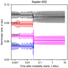 |
Fig. 3 N-body evolution of the semimajor axis, a, of the super-Earths in the compact system Kepler-402 as a function of time, t. The values of a of the planets are initialized to their current (observed) value. The solid curves indicate the semimajor axes. The envelopes are the periapses and apoapses of the orbits. Upon instability, planet b merges with planet c and planet d merges with planet e by giant impacts. No planet becomes metal rich in this simulation, but a different outcome is possible for different initial eccentricities and mean longitudes. |
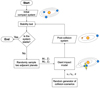 |
Fig. 4 Flowchart of the statistical model of orbital instability. For details on each step, see Section 2.2.2. The symbols MT and MP indicate the masses of the target and projectile in the collisions, respectively. The symbols ZT and ZP indicate the core-mass fractions of the target and projectile of the collisions, respectively. The distributions from which the relative impact velocity, v∞ (in units of Keplerian velocity, vk) and impact angle, θ, are sampled are shown in Figure B.1c, d. |
2.2.3 Collision model
To model giant impacts in planet-formation models, Emsenhuber et al. (2020) and Cambioni et al. (2021) showed that one needs to know at least seven impact outcomes: (1) the mass balance between remnants; (2) the mass-frequency distribution of smaller debris; (3) the composition of the largest remnant; (4) the composition of any escaping projectile; the (5) energy, (6) post-collision impact parameter and (7) argument of the pericenter of the relative orbit of any escaping projectile. To predict these quantities, we designed seven corresponding neural networks, gi (i = 1,...,7), that approximate the giant-impacts outcomes yi (i = 1,...,7):
 (7)
as a function of the array of impact conditions, x, whose elements are: logarithm of the target’s mass, MT ; logarithm of the projectile’s mass, MP; core-mass fractions of target and projectile, ZT and ZP respectively; vcoll/vesc; and the sine of the impact angle, θ. The impact outcomes yi are: the accretion efficiencies of the collision, ξL = (ML − MT)/MP and ξS = (MS − MP)/MP, where ML and MS are the masses of the largest remnant and any escaping projectile in hit-and-run collisions (the latter is termed “second-largest remnant” hereafter; we declare a collision to be a hit-and-run if MS > 0.1MP as in previous studies; Emsenhuber et al. 2020); the core-mass fractions of the largest remnant and any second-largest remnant, ZL and ZS respectively; the specific energy, ϵ′, post-collision impact parameter, b′, and variation of the argument of pericenter, △ω′, of the egress hyperbolic relative orbit of any second-largest remnant, as in Emsenhuber et al. (2020); the power-law index, β, of the mass-frequency distribution for debris smaller than the two largest remnants, and the mass fraction of largest debris body, ξd, computed over a total debris mass MD = MT + MP − ML − MS . Giant impacts with MP < 0.05MT or MT < 10−4 M⊕ are modeled as perfectly inelastic. Note that the seven neural networks of Equation (7) also maximize prediction accuracy because they are equivariant to the choice of the units system (Villar et al. 2023).
(7)
as a function of the array of impact conditions, x, whose elements are: logarithm of the target’s mass, MT ; logarithm of the projectile’s mass, MP; core-mass fractions of target and projectile, ZT and ZP respectively; vcoll/vesc; and the sine of the impact angle, θ. The impact outcomes yi are: the accretion efficiencies of the collision, ξL = (ML − MT)/MP and ξS = (MS − MP)/MP, where ML and MS are the masses of the largest remnant and any escaping projectile in hit-and-run collisions (the latter is termed “second-largest remnant” hereafter; we declare a collision to be a hit-and-run if MS > 0.1MP as in previous studies; Emsenhuber et al. 2020); the core-mass fractions of the largest remnant and any second-largest remnant, ZL and ZS respectively; the specific energy, ϵ′, post-collision impact parameter, b′, and variation of the argument of pericenter, △ω′, of the egress hyperbolic relative orbit of any second-largest remnant, as in Emsenhuber et al. (2020); the power-law index, β, of the mass-frequency distribution for debris smaller than the two largest remnants, and the mass fraction of largest debris body, ξd, computed over a total debris mass MD = MT + MP − ML − MS . Giant impacts with MP < 0.05MT or MT < 10−4 M⊕ are modeled as perfectly inelastic. Note that the seven neural networks of Equation (7) also maximize prediction accuracy because they are equivariant to the choice of the units system (Villar et al. 2023).
The networks were trained, validated, and tested using a look-up table of impact conditions and outcomes built by post-processing a state-of-the-art database of 1250 high-resolution SPH simulations of giant impacts from Emsenhuber et al. (2024). The colliding bodies in the dataset are planets differentiated into a fosterite mantle and an iron core whose Z varies between 0 and 1. The target’s mass spans six orders of magni- tude, from 10−4 to 5 M⊕. We used 70% of the table entries for training using the Adam algorithm (Kingma & Ba 2014). Another 15% of the table entries were used to identify the network architectures that do not overfit the training data by combining the following hyperparameters: learning rates of 0.002, 0.02, or 0.2; up to three hidden layers with 16, 32, 64, 128, or 256 neurons per layer; ReLu, Sigmoid, or Tanh activation functions; drop-out rates of 0.2%, 2%, or 20%; input normalization following the Standard, MinMax, or Robust scalings. To minimize overfitting, we operated batch normalization on the input layer and added Gaussian noise with strength 0.005 prior to the output layer. We used the remaining 15% of the table entries to assess the networks’ performance on unseen data in units of mean squared error (MSE) between the networks’ predictions and the SPH predictions. Using this procedure, we generated 66 295 converged neural networks, from which we chose the optimal networks gi(i = 1,...,7) as those that do not overfit the training data and have the lowest MSE at testing (Figure C.1 and Supplementary Dataset S2). These networks generalize well to the prediction of the giant-impact outcomes at testing, with correlation coefficients >89%.
We trained the neural networks on the SPH database of Emsenhuber et al. (2024) because, to our knowledge, it is state-of-the-art in terms of the variety of impact conditions and size of the parameter space explored. Note, however, that the SPH simulations in the database do not uniformly cover the parameter space, especially not the highly erosive regions, and do not include targets with MT > 5 M⊕. Despite this, we find that the networks g1 and g3 accurately extrapolate ξL and ZL for MT > 5 M (that is, the upper limit of the training database) with MSEs equal to 0.01 and 0.02, respectively, which are comparable to the SPH numerical noise level (Emsenhuber et al. 2024). Here the MSEs were computed between ξL and ZL from networks g1 and g3 and L and ZL predicted by Reinhardt et al. (2022), who modeled catastrophic disruption of super-Earths by impacts using a different SPH code than Emsenhuber et al. (2024). For this comparison, we assumed MT between 1 and 20 M⊕, θ = 0°, ZT = ZP = 0.3, MT = MP, and explored impact energies between 0 and 2 times the energy for catastrophic disruption computed using Equations (A.1) and (A.3) from Movshovitz et al. (2016).
We implemented the neural networks in a collision resolver which improves upon our previous work (Cambioni et al. 2019; Emsenhuber et al. 2020; Cambioni et al. 2021) by including explicit production and orbital evolution of debris smaller than the second-largest remnant and self-consistent evolution of planetary core-mass fractions in impact chains. Based on ML, MS , ZL, and ZS , the collision resolver predicts the radius of the impact remnants using a interpolating function based on the masses, radii, and core-mass fractions of the initial SPH bodies in the database by Emsenhuber et al. (2024). For the debris, the collision resolver computes MD and the metal content of debris, ZD, by imposing conservation of mass. If ZD > 1 due to accumulation of numerical errors, then ZD is randomly sampled from a Rayleigh distribution with scale value of 0.1 to account for the prediction by Cambioni et al. (2021) that ~85% of giant-impact debris are composed of mantle materials and ZL and ZS are updated by imposing conservation of mass.
The way we model the orbital evolution of debris depends on the value of vcoll. If vcoll ≲ 2 vesc, giant impacts tend to produce sizable debris fragments whose orbits can be reliably fit by the SPH simulator (Emsenhuber et al. 2024). In this circumstance, we add two debris bodies with masses Md1 > Md2 > 10−4 M⊕ and metal fractions Zd1 = Md1/MD ZD and Zd2 = Md2/MD ZD to the post-collision planetary population and assume that the remaining debris mass is accreted by the largest remnant. Masses Md1 and Md2 are randomly sampled from the mass-frequency distribution predicted by the neural network g2(x). The clumps are ejected radially from the edge of the largest remnant’s Hill sphere with v∞ = 0.5 vcoll following Emsenhuber et al. (2024).
If instead vcoll ≳ 2 vesc, we make the simplifying assumption that the largest remnant re-accretes the whole debris mass because of two reasons. First, these collisions produce unresolved debris whose mass-frequency distribution cannot be reliably assessed from SPH simulations and thus predicted by our neural networks. Second, a significant fraction of these unresolved debris is expected to be reaccreted by the target relatively quickly. For example, a Mercury-sized target is estimated to reaccrete one-third of its mantle ejecta in <2 Myr (Gladman & Coffey 2009), and we may expect a higher accretion rate for super-Earths owing to their higher gravitational focusing and lower orbital periods. Note, however, that the assumption that the target accretes all debris if vcoll ≳ 2 vesc could artificially lower the mantle-stripping efficiency. We therefore test the robustness of our results to this assumption in the Result Section 3.2.
2.3 Compact systems: Observations and model assumptions
2.3.1 Nominal scenario
To initialize the model of orbital instability of compact systems described in Section 2.2.2, we built a dataset of observed compact systems by searching in the NASA Exoplanet Archive for planetary systems containing multiple planets with orbital periods between 1 day and 1 year. We limited our search to planets around single stars and that have a terrestrial composition (defined as having R0 < 2R⊕, see Section 2.1.2; hereafter, we use the subscript “0” to indicate the properties of the super-Earths in the compact systems before the instability.) This assumption is supported by the observation that 70% of planets in the systems with high-density exoplanets are terrestrial planets (Figure D.1; see also discussion in Section 3.2).
If the mass of a super-Earth in these compact systems, M0, is unknown or known with σM0 /M0 > 30%, we set the planet’s initial core-mass fraction, Z0, to be 0.33. This value corresponds to a bulk composition with the average local galactic abundance of iron and rock-forming elements (Figure 2). Otherwise, we derived Z0 from the observed radius, R0, and M0 using the interpolation function based on the pre-impact bodies of the SPH simulations used to train the collision model of Section 2.2.3. This approach enables us to self-consistently evolve the core-mass fraction of planets undergoing collision chains, as the neural networks were trained on the same SPH simulations. We estimate that the relative difference between the radius predicted by this simplified model and that predicted by the well-established interior model by Zeng et al. (2021) is lower than 7%, similar to the typical measurement uncertainty of exoplanet radii (≲8%; Otegi et al. 2020; Luque & Pallé 2022; Parc et al. 2024). We rejected those systems in which at least one planet is a water-rich world or a high-density world (that is, if there are planets with density outside the nominal rocky planet zone defined by Unterborn et al. 2023). The catalog of compact systems is the Supplementary Dataset S3 and the cumulative distributions of the masses and radii of the super-Earths in the compact systems are plotted in Figure B.1a, b.
In our nominal scenario N0, we assumed that the precursor systems of the observed high-density exoplanets are well represented by the compact systems in Dataset S3 (we provide evidence supporting this assumption in Section 3.1). For the collision model, we randomly sampled the value of χ [which defines v∞ and thus vcoll given vK and vesc, Equations (1) and (6)] from its probability distribution derived from previously published results of N-body simulations by Volk & Gladman (2015), who evolved the orbits of selected compact systems until they experienced collisions. In addition, we randomly sampled the impact angle θ from the differential probability dP(θ) = sin(2θ) dθ, which yields a most likely θ of 45°. This probability function was first derived by Gilbert (1893) from the geometric argument that the differential probability that a point-mass impactor would hit a massless spherical target at a distance x = RT sin θ from its center is dP(θ) = 2π x dx. It was later shown that the proportionality dP(θ) ∝ sin 2θ holds when the gravity of the largest body is included (Shoemaker 1962). This result is expected to hold for giant impacts too (Asphaug 2010). We refer to Gabriel & Cambioni (2023) for a full derivation of dP(θ).
2.3.2 Variations of the nominal scenario
Because the properties and dynamical environment of the pre-cursor planetary systems are a priori unknown, we explored variations of the nominal scenario aimed at encompassing a large diversity of scenarios and corresponding model parameters. Each scenario described below is identical to the nominal scenario except for one parameter.
T1: In this scenario, we excluded from the catalog of precursor systems those systems that have two initial planets, which some studies have suggested might be the descendants of more closely packed planetary systems that already experienced instability (Pu & Wu 2015; Volk & Gladman 2015);
T2: In this scenario, we assumed that the super-Earths in the precursor systems whose mass is unknown or poorly constrained (σM0 /M0 > 30%) are metal-poorer than in the nominal scenario. As such, we initialized the masses of these super-Earths assuming Z0 = 0.2, which corresponds to an iron content one standard deviation below the average galactic value (Figure 2);
T3: In this scenario, we assumed that the super-Earths in the precursor systems whose mass is unknown or poorly constrained (σM0 /M0 > 30%) are more metal-rich than in the nominal scenario. As such, we initialized the masses of these super-Earths assuming Z0 = 0.4, which corresponds to an iron content one standard deviation above the average galactic value (Figure 2);
T4: In this scenario, we assumed that the probability distribution of χ = v∞ /vk follows a Rayleigh distribution with a scale value of 0.1, corresponding to a lower degree of dynamical excitation than in the nominal scenario (Figure B.1c). We assume a Rayleigh function because this was found to well represent the distribution of impact velocities for planetary systems that experience orbit crossings (Gabriel & Cambioni 2023);
T5: In this scenario, we assumed that the probability distribution of χ = v∞/vk follows a Rayleigh distribution with a scale value of 0.4, corresponding to a higher degree of dynamical excitation that in the nominal scenario (Figure B.1c);
T6: In this scenario, we relaxed our assumption that every super-Earth in the precursor systems must have R0 < 2R⊕ and allowed planets with 2 R⊕ < R0 < 3 R⊕ into the sample. This scenario is motivated by the recent detection of planets with radii between 2 and 3 R⊕ and densities consistent with a volatile-poor composition (Otegi et al. 2020). Based on this, we found 12 additional precursor systems and explored their stability and collisional evolution using our statistical model.
2.4 Comparison with observed high-density exoplanets
We compared the simulated metal-rich worlds with the observed high-density exoplanets using three metrics: (1) predicted versus observed occurrence rate; (2) similarity between the modeled versus observed mass-radius distributions; and (3) the rate at which giant impacts can form metal-rich worlds as massive and large as the observed high-density exoplanets.
2.4.1 Predicted occurrence rate
We computed the occurrence rate of simulated metal-rich planets formed in our model of orbital instability, ηMR, as their fraction in the post-instability planetary population. We correct ηMR for typical biases in the exoplanetary population as
 (8)
where n is the number of simulated metal-rich planets, ntot is the total number of post-instability planets, and pSurvey is the probability that transiting planets with R and orbital period as the simulated metal-rich planets are classified as reliable planet candidates. We calculate pSurvey using the Kepler Exoplanet Population Observation Simulator (Mulders et al. 2019) for stars more massive than 0.6 solar masses and the Transiting Exoplanet Survey Satellite likelihood model (Ballard 2019) otherwise. We estimated the predicted number of metal-rich planets in the terrestrial planet population as the number of terrestrial planets in Dataset S1 times
(8)
where n is the number of simulated metal-rich planets, ntot is the total number of post-instability planets, and pSurvey is the probability that transiting planets with R and orbital period as the simulated metal-rich planets are classified as reliable planet candidates. We calculate pSurvey using the Kepler Exoplanet Population Observation Simulator (Mulders et al. 2019) for stars more massive than 0.6 solar masses and the Transiting Exoplanet Survey Satellite likelihood model (Ballard 2019) otherwise. We estimated the predicted number of metal-rich planets in the terrestrial planet population as the number of terrestrial planets in Dataset S1 times  .
.
2.4.2 Similarity of mass–radius distributions
We tested the null hypothesis that the population of observed high-density exoplanets as a whole formed by mantle-stripping giant impacts using the two-dimensional Kolmogorov–Smirnov (KS) test. This test assesses whether the mass-radius distributions of the simulated metal-rich worlds and that of the observed high-density exoplanets are drawn from the same underlying distribution. For this test, we built the mass-radius distribution for the simulated metal-rich planets by randomly sampling the (M, R) values of two thirds of metal-rich planets from the model population with weights equal to pSurvey, without replacement. We estimated the mass-radius distribution of the observed high-density exoplanets by bootstrapping 1000 (M, R) values for each planet within uncertainties.
2.4.3 Rate of formation of metal-rich worlds akin to the observed high-density exoplanets
The KS analysis of Section 2.4.2 is meant to test the null hypothesis that mantle stripping by giant impacts is the predominant pathway through which the population of high-density exoplanets form. However, even in case of the KS test rejects this null hypothesis, it is still possible that some of the observed high-density exoplanets formed through mantle-stripping giant impacts. To investigate this, we computed the rate pGI at which a given scenario among those described in Section 2.3.1 form simulated metal-rich worlds with M and R similar to each of the observed high-density exoplanets. We compute pGI as the fraction of simulated metal-rich worlds with M and R within the three–standard-deviation uncertainty ellipse of the M and R of the observed high-density exoplanets.
3 Results and discussion
3.1 Instability of compact systems
We find that 29±17% of the precursor compact systems can become unstable within 10–100 Myr and thus experience orbit crossing and possibly a phase of giant impacts. In the nominal scenario N0, only ~20% of the stable compact systems show near–mean-motion resonances between planetary pairs (Figure E.1), consistent with the general paucity of resonances and near-resonance features observed across compact systems (Weiss et al. 2023, for a review). Importantly, in the nebular phase of planet formation, planet-disk interactions can lead planets to experience orbital migration, which if convergent may naturally shepherd planets into mean-motion resonances (e.g., Batygin 2015). As such, the lack of resonances in the stable compact systems in our dataset suggests that these systems are stable today either because they escaped resonance during the nebular period or experienced an orbital instability after nebular gas dissipation (Goldreich & Schlichting 2014; Izidoro et al. 2017, 2021; Matsumoto & Ogihara 2020). By contrast, we find that 70% of the compact systems that we predict to become unstable have at least a pair of super-Earths in near–mean-motion resonances (Figure E.1). This suggests that at least 70% of the compact systems in our catalog whose instability can form metal-rich planets are likely to be primordial (that is, they did not experience an instability yet). This builds confidence in our assumption that the majority of the unstable compact systems are representative of the possible precursor systems of the observed high-density exoplanets.
3.2 Giant-impact outcomes
Across all scenarios in Section 2.3.1, we record 109 unstable system configurations (Table F.1). For each unstable configuration, we used the statistical model described in Section 2.2 to simulate their orbital and collisional evolution for 1000 different scenarios, for a total of 109 1000 = 109 000 different cases.
In most of these collision scenarios, the super-Earths in the compact systems merge to form larger planets without a significant change in metal content, potentially explaining the detection of planets with an Earth-like interior structure above the radius-gap valley (Essack et al. 2023; Naponiello et al. 2023). In some other cases, the super-Earths experience chains of ~2–3 collisions that strip their mantles, causing them to evolve into metal-rich, high-density planets (Figures 5). The giant impacts that form the simulated metal-rich planets are hit-and-run collisions in 99% of the cases. In these events, a projectile super-Earth grazes a larger target super-Earth and continues along a deflected stellocentric orbit as a metal-rich planet distinct from the target (Figure 6; Movie S1). The escaping projectile avoids reaccreting its own debris because its mantle is mostly accreted by the target following the collision. This scenario is analogous to the hit-and-run theory proposed to explain the anomalously large metallic core of planet Mercury (Asphaug & Reufer 2014), with the difference that, in our model, the giant impacts involve super-Earths and occur at smaller stellocentric distances.
We now discuss the robustness of this finding to model assumptions. First, we investigate whether the finding that targets that become metal-rich giant-impact remnants are exceedingly rare is a model artifact due to the assumption that targets accrete all the unresolved debris for collisions at vcoll ≳ 2 vesc (Section 2.2.2). We find that our finding is robust to this assumption because the vast majority of the collisions (92%; Figure G.1) in our simulations occur at vcoll ≲ 2 vesc, for which our model explicitly simulates the orbital evolution of debris.
Second, we assess the robustness of our results against the assumption that all colliding bodies are super-Earths by investigating the likelihood that a super-Earth projectile would lose its mantle in a hit-and-run collision onto a gas-rich target. In our simulations, we assumed that collisions occur between super-Earths with no gaseous envelopes (Section 2.3.1). However, in compact planetary systems, super-Earths can have sub-Neptune companions too (Weiss et al. 2023). Indeed, five of the high-density exoplanets listed in Table 1 have transiting sub-Neptune companions (TOI-1468 b, TOI-431 b, HIP-29442 d, Kepler-107 c, and Kepler-80 d, Figure D.1).
For different collision velocities, we compare the outcome of impacts between a super-Earth projectile onto a sub-Neptune with a 1.67 M⊕ iron core, 3.33 M⊕ rocky mantle, and 1.25 M⊕ hydrogen atmosphere to the predictions for the same collisions assuming that the target is a larger super-Earth [the predictions are based on the SPH simulations from Denman et al. (2022) and our machine-learning model of giant impacts, respectively]. The results are in Figure 7a, which plots the density of the surviving hit-and-run projectile (ρS, in units of  defined in Section 2.1) as a function of vcoll for the two different scenarios with projectile mass MP = 1 and 3 M⊕. Over the same range of vcoll, we find that
  is above the high-density threshold [dashed red line, Equation (3)] if the target is a super-Earth, while it is below the threshold if the target is a sub-Neptune. This indicates that erosion of mantle materials in impacts onto atmosphere-rich sub-Neptune-sized planets is less efficient than direct impact onto solid super–Earth-sized targets. As discussed in Denman et al. (2022), the target’s atmosphere is eroded preferentially to the projectile’s mantle for two reasons. First, the atmosphere is significantly less gravitationally tightly bound than the mantle material, so that it can escape more easily. Second, the impedance mismatch between atmosphere and mantle means that any shock waves in the projectile’s mantle caused by atmospheric shocks are substantially weaker than the initial shock that caused them, which frustrates mantle stripping.
Higher impact energies than those achieved in collisions between a super-Earth and a sub-Neptune could be achieved if a super-Earth collides onto a Jupiter-sized planet. However, formation of a metal-rich world in this scenario is unlikely for two reasons. First, as the projectile-to-target radius ratio decreases, the super-Earth projectile would need to graze its Jupiter-sized target at an impact angle θ > 60° to be stripped of its mantle and avoid being accreted (Figure 7b). However, the most likely impact angle is θ = 45°, and there is only 25% probability that θ > 60° (Section 2.3.1 and Figure B.1d). In addition, no observed high-density exoplanet has a detected Jupiter-sized companion (Figure D.1), but this can be the result of observational bias.
Overall, we conclude that a super-Earth is more likely to evolve into and survive as a metal-rich world in a hit-and-run collision if the target is a similar-sized super-Earth. This suggests that our results are robust against the assumption that all colliding bodies are planets of terrestrial composition.
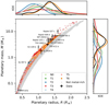 |
Fig. 5 Results from our orbital instability model for different model assumptions. Mass, M, as a function of radius, R, of the simulated planets surviving an orbital instability for the different model assumptions described in Section 2.3.1. The final planets are deemed metal-rich remnants (colored symbols) and non-metal-rich remnants (gray symbols) based on the high-density threshold of Equation (3). The black data points correspond to the observed high-density exoplanets listed in Table 1, with one standard deviation uncertainty bars; planet Mercury is plotted for comparison. The side plots are the Kernel Density Estimates (KDEs) of the radius (top) and mass (left) of the observed high-density planets (black curve) and the simulated metal-rich giant-impact remnants (colored curves). The model KDEs are weighted according to the probability of detection of the simulated metal-rich worlds by transit surveys, to mimic observational bias typical of exoplanetary surveys (Section 2.4). |
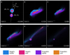 |
Fig. 6 Hit-and-run collision between two super-Earths forming a metal-rich planet. Panels a through f: snapshots of a SPH simulation of a giant impact (times after collision listed at lower right each panel) from the dataset by Emsenhuber et al. (2024). The target body has mass MT = 2.5 M⊕ and core-mass fraction ZT = 0.30; particles composing the mantle and core of the target are colored in blue and red, respectively. The projectile has mass MP = 1 M⊕ and core-mass fraction ZP = 0.16; particles composing the mantle and core of the projectile are colored in purple and orange, respectively. The collision velocity is vcoll = 2.54 vesc and the impact angle is θ = 15° [see definitions in panel (a)]. Note scale bars at lower left. The projectile’s mantle is accreted by the target, while the projectile’s core escapes as a metal-rich planet. For an animation of this SPH simulation, see online Movie S1. |
3.3 Effect of parent-body size on mantle stripping
The radius of the simulated metal-rich planets, R, ranges from R ≈ 0.2 R⊕, smaller than planet Mercury and GJ 367 b, to R ≈ 2.2 R⊕, larger than all observed high-density exoplanets listed in Table 1 (Figures 5). This indicates that mantle-stripping giant impacts between super-Earths can form metal-rich worlds as large as the observed high-density exoplanets.
Nevertheless, we also find that most simulated metal-rich planets are Earth-sized or smaller. Specifically, 95% of all simulated metal-rich worlds have radii smaller than R95 = 1.2 R⊕ in the nominal scenario. Notably, the value of R95 varies from 1.0 to 1.6 R⊕ across the different scenarios considered (a summary of the results is in Table F.1). The minimum R95 is recorded for the scenarios in which super-Earths have a lower metal content than the nominal scenario (T2). The maximum is recorded for the scenarios in which super-Earths have a higher metal content than the nominal scenario (T3) or if the precursor systems have super-Earths with R0 = 2–3R⊕ (T6). Assuming that the nominal case and the other cases are all equally probable, we average the 109 000 simulation results and obtain R95 = 1.3 ° 0.2 R⊕, where the uncertainty corresponds to one standard deviation.
We investigated whether the preferentially sub-Earth size of the simulated metal-rich worlds is due to their parent bodies being super-Earths with R0 < 2–3 R⊕ (Figure B.1a and Section 2.1.2). To test this, for a given super-Earth of size R0, mass M0, and core-mass fraction Z0 that becomes metal-rich in at least one simulation from our statistical model, we randomly sampled a core-mass fraction, Z, between Z0 and 1 and estimated the corresponding post-impact mass as M ~ Z0/Z × M0. We find that the simulated metal-rich planets have a radius distribution that is consistent with that of this randomly eroded population (Figure 8a). This indicates that the size of the simulated metal-rich planets is indeed limited, at least in part, by that of their parent bodies.
However, we also find that the simulated metal-rich planets from the model of orbital instabilities tend to have a lower mass, M (or equivalently, a lower density for a given R), than the metal-rich planets of the randomly eroded population (Figure 8b). This suggests that the size distribution of the simulated metal-rich worlds is also affected by the binding energy of their parent super-Earths, which opposes their impact disruption (e.g., Movshovitz et al. 2016). Because binding energy increases with increasing planetary size (e.g., Gabriel & Cambioni 2023), the percentage of mantle erosion is expected to decrease with increasing planetary size for a given range of v∞. Consistent with this, we find that the probability that a super-Earth suffers mantle stripping decreases with R0 (Figure 8c), dropping from ~50% to ≲5% for R0 < 1 R⊕ and R0 > 2 R⊕ respectively.
In addition, astronomical observations suggest that the spacing between adjacent planets in compact systems increases with planetary size (Mishra et al. 2021; Weiss et al. 2023) and that their mutual eccentricities are generally smaller than 0.1 (Hadden & Lithwick 2017). Because the likelihood of instability tends to decrease with increasing inter-planetary distances (Pu & Wu 2015), compact systems with larger planets may be inherently less likely to experience instability than systems with smaller planets. Consistent with this, in our results, we find that the fraction of precursor systems that experience instability appears to decrease with the median value of the initial size of their planets,  (Figure 8d).
Based on this, we propose that the preferential sub-Earth size of the simulated metal-rich giant-impact remnants can be explained as the result of three factors: the size of their parent super-Earths is in most cases smaller than 2 R⊕; the efficiency of mantle stripping is a decreasing function of planetary size; and the likelihood of compact system instability is a decreasing function of the average sizes of the planets in the compact systems.
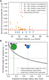 |
Fig. 7 Comparison of giant impacts among atmosphereless super-Earths to collisions involving atmosphere-rich targets. (a) Density of the surviving hit-and-run projectile, ρS, as a function of vcoll. The value of ρS is plotted in units of |

3.4 Implications for the origin of metal-rich worlds
Our results demonstrate that super-Earths can become metal-rich planets by losing their mantles in giant impacts. However, we also find that the formation of metal-rich giant-impact remnants is a rare occurrence, with a predicted observed occurrence rate among the terrestrial exoplanets in the post-instability population of  (that is, within error of zero), where the uncertainty is one standard deviation [Equation (8) in Section 2.4.1; Table F.1]. This is much lower than the occurrence rate of the observed high-density exoplanets (ηHD = 9%, Section 2.1.2). When scaled to the number of observed terrestrial exoplanets,
  translates to at most one out of the 12 observed high-density exoplanets being a metal-rich giant-impact remnant. Importantly, our estimated
  is most likely an upper limit for two reasons. First, we are overestimating the number of metal-rich worlds by assuming that all unstable compact systems will undergo a phase of giant impacts. Second, we are underestimating the total number of terrestrial exoplanets by considering only exoplanets in the post-instability populations. In reality, not all unstable systems would undergo giant impacts to achieve stability and not all systems with terrestrial planets would experience an instability.
Following the procedure outlined in Section 2.4.2, we find that the mass-radius distribution of the simulated metal-rich worlds corrected for observational biases has KS probability smaller than 5×10⁻¹⁵ to be drawn from the same underlying distribution as that of the observed high-density exoplanets. This mismatch can be explained by most of the observed high-density exoplanets being larger and more massive than the simulated metal-rich worlds (Section 3.3). Consistently, we find that all scenarios (except T6, discussed below) form metal-rich worlds as large and massive as the observed high-density exoplanets only in pGI < 15% of the cases (Figure 9a). The exception is the observed high-density exoplanet GJ 3929 b, for which pGI = 20–40% depending on the scenario. This can be explained by GJ 3929 b having the lowest probability of being high-density among the observed high-density exoplanets (Table 1), making it easier to form via mantle stripping starting from a Z0 between 0.2 and 0.4.
The exception to the above trend in pGI is scenario T6, in which we explore the orbital instability of compact systems that have planets with R0 = 2–3 R⊕, thus larger than the maximum size of 2 R⊕ adopted in the nominal scenario. This scenario yields pGI > 20% for the high-density exoplanets of sizes between GJ 3929 b and Kepler-80 d (that is, from ~ 1 R⊕ to 1.5 R⊕), with a maximum pGI ~ 47% for Kepler-105 c. We explain the presence of a peak in pGI (Figure 9a) as being due to ~90% of the initial super-Earths in the scenario T6 being larger than 1 R⊕ (Figure B.1b). The lack of sub-Earth-sized planets in the precursor systems results in reduced collisional grinding at small scales. At the same time, the largest super-Earths in this scenario are too large for giant impacts to efficiently erode their mantles (Figure 8c). The competing factors of lack of bodies to grind down at small scales and reduced collisional grinding at large scales create a peak in the abundance of simulated metal-rich worlds at an intermediate size. Intriguingly, the one-dimensional probability density functions of masses and radii of the simulated metal-rich planets from scenario T6 visually resemble those of the observed high-density exoplanets (Figure 5). This makes scenario T6 the best-fit scenario among those tested to form metal-rich worlds akin to the observed high-density exoplanets.
Despite this, the formation of metal-rich worlds in scenario T6 remains a rare event, yielding a predicted observed occurrence rate  among terrestrial planets (Table F.1), thus lower than the occurrence rate of observed high-density exoplanets. Moreover, scenario T6 does not pass the KS test, neither in the two-dimensional (mass–radius) space nor if the one-dimensional probability mass and radius density functions of the simulated versus modeled planets are separately compared. Finally, the compact systems of scenario T6 are relatively rare, accounting for ~14% of all compact systems in the catalog (Appendix H), although it is possible that more of these systems could have existed in the past than are observed today. As such, we conclude that it is unlikely that scenario T6 can explain all the observed high-density exoplanets, although we cannot rule out that it can explain some of the observed high-density exoplanets of size 1–1.5 R⊕.
While super–Earth-sized metal-rich worlds rarely form by giant impacts during a late orbital instability, we predict sub-Earth-sized metal-rich worlds to be a relatively common outcome of such a process. This is shown in Figure 9b, where we binned the occurrence rate of metal-rich giant-impact remnants, ηMR (defined in Section 2.4.1), as a function planetary radius, R. Intriguingly, we estimate ηMR ~ 21 ± 12% for sub- Earth-sized planets, which supports the proposal that planet Mercury and some asteroids could be metal-rich giant-impact remnants (Asphaug & Reufer 2014; Volk & Gladman 2015; Elkins-Tanton et al. 2022). Note that the estimated ηMR exclusively concerns metal-rich worlds formed during a late orbital instability and does not include any Mercury-like planets that could have formed by giant impacts during the era of terrestrial planet formation. Finally, Figure 9b also show that ηMR is a monotonically decreasing function of R, consistent with our proposal that smaller planets are more likely to lose their mantle in giant impacts (Section 3.3).
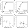 |
Fig. 8 Likelihood that mantle-stripping giant impacts occur as a function of size of the colliding bodies. (a) Cumulative distribution of the radii, R, of the simulated metal-rich planets compared to that of the corresponding randomly eroded population generated as described in Section 3.3. (b) Same as panel a, but for planetary masses, M. (c) Fraction of initial super-Earths in unstable compact systems that evolve into metal-rich planets (i.e., probability of mantle stripping) as a function of their initial size, R0. (d) Fraction of compact systems that experienced instability (i.e., probability of system instability) as a function of the median initial planetary size, |


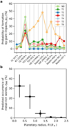 |
Fig. 9 Implications of our results for the formation of metal-rich worlds. (a) Probability pGI that a late orbital instability forms metal-rich worlds as large and massive as the observed high-density exoplanets. The probability is computed as described in Section 2.4 and the planets are listed along the x-axis in order of increasing size. (b) Occurrence rate of the modeled metal-rich giant-impact remnants, ηMR, binned as a function of planetary radius, R. ηMR is computed as the fraction of the metal-rich worlds in the post-instability planetary population; the vertical bars indicate one standard deviation uncertainties computed across all simulation scenarios described in Table F.1. While most of the observed high-density exoplanets are too large to be metal-rich giant-impact remnants, sub-Earth-sized metal-rich worlds formed during a late orbital instabilities should be instead relatively common in the local galaxy but are likely too small to be detected by current exoplanetary surveys. |
4 Conclusion
High-density worlds are a recently recognized compositional class of planetary objects whose density is far higher than what expected from cosmochemistry and whose sizes range from metal-rich asteroids to super–Earth-sized planets. In this work, we tested the hypothesis that the largest members of this population (the high-density exoplanets) are the metallic cores of super-Earths that lost their rocky mantles by giant impacts.
To test this hypothesis, we combined exoplanetary observations, orbital dynamics, collisional physics, and machine learning to develop and run a statistical model of orbital instability and collisional evolution of super-Earth systems. In our simulations, we maximized the likelihood of forming metal-rich worlds by giant impacts by studying the case in which the orbital instabilities involve close-in super-Earths that are tightly packed in compact systems around a host star. This scenario maximizes both the impact energies (Section 1) and the likelihood that one of the two colliding planets survives as a metal-rich world (Section 3.2). We explored a comprehensive set of scenarios (109 000 different coupled orbital-collisional simulations) by varying the initial composition, mass, and the degree of orbital excitation of the super-Earths in about 100 observed compact systems. Next, we compared the simulation results in terms of mass, radii, and occurrence rate of simulated metal-rich worlds to those of the observed high-density exoplanets.
Our study makes several assumptions and simplifications. First, we assumed that the observed compact systems are representative of putative precursor systems of the high-density exoplanets. This assumption is supported by our observation that ~70% of the unstable compact systems in our catalog have planets in near–mean-motion resonances, as expected for primordial systems that did not undergo instability (Section 3.1). Studies of the dynamical stability of multi-planet systems also show that there is significant overlap between the architectures (e.g., dynamical spacings, orbital period ratios, and mass ratios of nearest-neighbor planets) of systems that become unstable in numerical integrations and those that do not (e.g., Volk & Malhotra 2024). These instabilities also occur over a wide range of timescales (between ~103 and ~5 × 10⁹ orbital periods of the innermost planets), even for very similar initial mass-radius distributions and orbital periods of the planets (Volk & Malhotra 2024), which could be consistent with the argument that the observed compact systems are merely metastable (e.g., Volk & Gladman 2015). Consistently, we show that our results are largely insensitive to the orbital properties of the compact systems (tests T1, T4, T5, and T6; Section 2.3.2 and Figures 5). Nevertheless, it is possible that the architecture of the true precursor compact systems is not represented in our catalog.
Second, we calculated the observed occurrence rate based on a small sample of terrestrial planets that may be incomplete. We corrected the occurrence rate for two outstanding biases in Sections 2.1.2 and 2.4, but further analysis of the exoplanetary dataset is warranted. Third, our machine learning of giant impacts is trained on the SPH database by Emsenhuber et al. (2024). While we consider this database the state-of-the-art, it unevenly samples the parameter space of erosive collisions and limits the total collision masses to less than 10 M⊕. We show in Section 2.2.3 that these limitations are unlikely to affect the reliability of our results, as our predictions match those from an independent dataset of SPH simulations of catastrophic disruption of super-Earths up to 20 M⊕. However, the latter is limited to head-on collisions. As such, additional SPH simulations would be helpful to further validate our model.
Under these assumptions, we found that metal-rich worlds as massive and large as the observed high-density exoplanets can form as a result of giant impacts between super-Earths during a late orbital instability. Their formation occurs via hit-and-run collisions, in which the metallic core of a projectile super-Earth manages to escape accretion onto a larger super-Earth target. In this process, the mantle of the projectile is blasted off and sequestered by the larger super-Earth target. This scenario is similar to what is proposed for planet Mercury (e.g., Asphaug & Reufer 2014).
Nevertheless, we also find that most giant impacts occurring during a late instability result in pairwise accretion of the colliding super-Earths, yielding a predicted observed occurrence rate for the simulated metal-rich worlds smaller than ~1% among terrestrial planets. By contrast, we estimate that the observed occurrence rate of high-density exoplanets is ~9%. In addition, the mass-radius distribution of the metal-rich worlds is statistically distinct from that of the observed high-density exoplanets, with Kolmogorov-Smirnoff probability smaller than 5 × 10⁻¹⁵. Consistently, at most 15% of the metal-rich worlds formed during instabilities are as large and massive as the observed high-density exoplanets.
Our findings are largely insensitive to our model assumptions (Section 2.3.2). The only exception is the scenario in which the parent bodies of the metal-rich worlds are rare super-Earths of terrestrial composition with radius of 2–3R⊕, intermediate between the radius typical of super-Earths and sub-Neptunes. The instability of these rare systems can produce larger metal-rich planets than in other scenarios, albeit still with a predicted observed occurrence rate in the order of 1%. Note that while an orbital instability of compact systems maximizes the likelihood that metal-rich giant-impact remnants form, not all unstable systems would undergo giant impacts to achieve stability and not all systems with terrestrial exoplanets would experience an instability. As such, our predicted rate with which orbital instabilities in compact systems can produce metal-rich giant-impact remnants constitutes an upper limit.
We conclude that mantle-stripping giant impacts between super-Earths can form metal-rich worlds as large as the observed high-density exoplanets, but these events occur at rates not sufficiently high to explain the typical size and abundance of the observed high-density exoplanets. Based on the current observed rate, this translates to at most one of the observed high-density exoplanets being a metal-rich giant-impact remnant. This planet may be GJ 3929b, whose density barely satisfies the high-density criterion of Equation (3), resulting in the highest probability to be a metal-rich giant-impact remnant (20–40% depending on the scenario).
Our results indicate that most high-density exoplanets are unlikely to be metal-rich giant-impact remnants. We offer possible alternative explanations for the nature of high-density exoplanets, based on whether we can trust their currently estimated occurrence rate of 9%. If future exoplanetary surveys were to confirm the current high-density exoplanet occurrence rate, then there would be only two remaining hypotheses likely to explain the detection of most high-density exoplanets: these planets are either primordial metal-rich worlds or the naked compressed cores of gas giants that lost their volatile envelopes (Johansen & Dorn 2022; Mocquet et al. 2014), with the latter being disfavored based on planetary interior models (Lin et al. 2025). If future surveys instead lower the occurrence rate down to less than 1–2% or discover substantially more large terrestrial planets akin to the parent bodies in Scenario T6, our results suggest that mantle-stripping giant impacts may still be a viable formation mechanism.
Finally, we find that the occurrence rate of metal-rich worlds forming from the orbital instability of compact systems is a monotonically decreasing function of planetary radius, owing to mantle stripping being more efficient for smaller planets (Figure 9b). Our simulations yield an occurrence rate of metal-rich giant-impact remnants smaller than Earth of 21 ± 12% among terrestrial exoplanets (1-σ uncertainty). As such, we predict that sub-Earth-sized metal-rich worlds should be relatively common in the galaxy but are likely too small to be detected by current exoplanetary surveys. The formation rate of these planets ranges between ~9 and ~43% across all our model realizations that assume an initial abundance of iron and rock-forming elements as that of CI carbonaceous chondrites. This finding supports the proposal that the planet Mercury and some metal-rich asteroids are metal-rich worlds that formed by giant impacts, without the need for a metal enrichment of the local protoplanetary disk (Asphaug & Reufer 2014; Volk & Gladman 2015; Elkins-Tanton et al. 2022).
Data availability
Datasets S1, S2, and S3 are available at https://doi.org/10.5281/zenodo.15058176 (Cambioni 2025).
The Movie associate to Fig. 6 is available at https://www.aanda.org
Acknowledgements
S.C. acknowledges funding from the Crosby Distinguished Postdoctoral Fellowship of Department of Earth, Atmospheric and Planetary Sciences, Massachusetts Institute of Technology (MIT). S. C. and B. P. W. acknowledge funding from NASA contract NNM16AA09, “Psyche: Journey to a Metal World.” K. V. acknowledges support from NASA (Exoplanets Research Program grants 80NSSC18K0397, 80NSSC20K0267, and “Alien Earths” grant 80NSSC21K0593); the results reported herein benefited from collaborations and/or information exchange within NASA’s Nexus for Exoplanet System Science (NExSS) research coordination network sponsored by NASA’s Science Mission Directorate. Z. L. acknowledges funding from the Center for Matter at Atomic Pressures (CMAP), a National Science Foundation (NSF) Physics Frontiers Center, under Award PHY-2020249. The authors acknowledge the MIT SuperCloud and Lincoln Laboratory Supercomputing Center for providing high-performance computing, database, and consultation resources.
Appendix A Estimation of the effect of the radial-velocity bias on ηHD
Most of the terrestrial exoplanets in our catalog (~90%) were discovered with the transit method (Dataset S1). In most cases, their discovery was later followed by mass measurements using the radial velocity (RV) method. The signal semi-amplitude of RV measurements, K, increases with M as
 (A.1)
where M* is the host star mass and I is the angle between the plane in which the planet orbits and the plane perpendicular to the line of sight. Because the mass of a high-density exoplanet is larger than that of a similarly sized planet with an Earth-like composition, the former has higher K than the latter assuming a similar orbital period. This may make it easier to detect or obtain better mass constraints on high-density exoplanets than of terrestrial planets, potentially leading to an overestimation of ηHD as computed in Section 2.1.2.
(A.1)
where M* is the host star mass and I is the angle between the plane in which the planet orbits and the plane perpendicular to the line of sight. Because the mass of a high-density exoplanet is larger than that of a similarly sized planet with an Earth-like composition, the former has higher K than the latter assuming a similar orbital period. This may make it easier to detect or obtain better mass constraints on high-density exoplanets than of terrestrial planets, potentially leading to an overestimation of ηHD as computed in Section 2.1.2.
Quantifying the correction factor for ηHD to account for this bias is not straightforward because P, M, M* (and to a lesser extent, I and e) are highly variable across the exoplanetary catalog. Furthermore, these values are a priori unknown for planets whose RV signal is below current detection limits. As such, here we limit ourselves to bound the effect of the RV bias on ηHD through two worst-case scenarios.
First, we assume that the RV bias always leads to larger uncertainties in the RV masses for less massive planets. To explore this, we redo our search for terrestrial exoplanets as described in Section 2.1.2, but assuming a more permissive σM/M < 0.5 instead of σM/M < 0.3. We still use the criteria σM/M < 0.3 for the high-density exoplanets. Second, we assume that the RV bias always leads to missed detections of terrestrial planets with an Earth-like composition, but never of similarly sized high-density exoplanets. To explore this, we build a synthetic population of 100 terrestrial exoplanets with Z = 0.30 and radii randomly sampled from the radius distribution of the high-density exoplanets in Table 1. We assume that the masses of these terrestrial planets can be constrained by the RV method if their K as defined by Equation (A.1) is greater than an assumed RV detection limit Kth. We explore how the number of detected terrestrial planets, NR, varies as a function of Kth between ~0.3 cm s−1 and 10 ms−1. The lowest value Kth is the best precision level achieved by the latest generation of spectrographs, while the highest value of Kth is ~100 times the velocity variation that the Earth produces on the Sun (Hara & Ford 2023, for a review). We assume I = 90°, e = 0, M* equal to 1 solar masses for all planets, and explore P = 1 day, 10 days, or 100 days.
The first test yields ηHD = 12/103 = 12% assuming that all terrestrial planets have R < 2R⊕ (Dataset S1). In the second test, we find (Figure A.1) that NR drops from 100% to 0% for Kth > 3.5, 2.0, and 1 ms−1 if P = 1, 10, and 100 days respectively. We note that 54%, 21%, and 2% of the observed terrestrial exoplanets in Dataset S1 have K > Kth = 3.5, 2.0, and 1 ms−1, respectively (histogram in Figure A.1). We therefore infer that at most 54% of the terrestrial planets may not have been detected due to the RV bias. This translates to a minimum ηHD of 9% assuming that the 12 high-density exoplanets are so massive to be detectable regardless of the value of Kth. The unbiased value of ηHD is still at least nine times larger that the predicted observed occurrence rate of the simulated metal-rich worlds ηMR ≲ 1% (Section 3.4). As such, we conclude that our results presented in the main text are robust to the RV bias as quantified here.
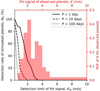 |
Fig. A.1 Effect of the radial-velocity bias on the detection of terrestrial planets. Left-bottom axes: Percent of terrestrial exoplanets detected, NR, as a function of the detection limit of RV signals, Kth, for different values of the orbital period P of the 100 terrestrial exoplanets in the model catalog. Right-top axes: Probability Density Function (PDF) of the RV signals of the observed terrestrial exoplanets in Dataset S1. |
Appendix B Input probability distributions for the orbital statistical model
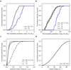 |
Fig. B.1 Input probability distributions for the orbital statistical model. a) Distribution of initial planets’ radius, R0, in the precursor compact systems whose properties are listed in Dataset S3. b) Distribution of initial planets’ mass, M0, in the compact systems (Dataset S3). c) Distribution of the relative impact velocity in units of Keplerian velocity, v∞/vk, assumed in the statistical model of Section 2.2.2. d) Distribution of the impact angle, θ assumed for the collision model in Section 2.2.2. The different curves are for the nominal case (N0) and the robustness tests (T1–T6). |
Appendix C Training, validation, and testing of the optimal neural networks in the giant-impact model
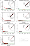 |
Fig. C.1 Training history and performance of the optimal neural networks composing the giant-impact model. Panels a–g: Mean squared error (MSE) between y(x) predicted by the neural networks gi(i = 1,...,7) and the corresponding SPH outcome, t(x), as a function of the training epochs. The inset plots show the correlation with index R between y(x) and t(x) for the testing set. The complete training report (including the suboptimal neural networks) is in the Dataset S2. |
Appendix D Demographics of systems with high-density exoplanets
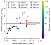 |
Fig. D.1 Radius, R, as a function of semimajor axis, a, of planets in the planetary systems where high-density exoplanets have been observed. The data points are color coded by their masses, M (in units of M⊕). We plot only planets for which the radius and masses are known with sufficient precision to enable compositional estimates, i.e., σR/R <0.3 and σM/M <0.3. We distinguish between terrestrial planets (symbols with black edges) and volatile-rich planets (symbols with red edges) based on whether their R is greater or smaller than 2 R⊕, respectively (see Section 2.1.2). Most of the known planets in the systems with high-density exoplanets are predominantly made of rock and iron, with no large volatile envelopes. |
Appendix E Period ratios of planets in the precursor compact systems
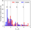 |
Fig. E.1 Histograms of the period ratios of planets in compact systems. We distinguish between compact systems that are stable and likely to become unstable within the next 10–100 Myr following the procedure outlined in Section 2.2.2 (red and blue histograms, respectively). In the stable systems, we find that 30% of the planetary pairs are within 0.1 Pj+1/Pj of mean-motion resonances (7%, 15%, 4%, and 5% have period ratios 3:2, 2:1, 3:1, and 4:1 respectively). In the systems that we predict to be unstable, we find that 50% of the planetary pairs are within 0.1 Pj+1/Pj of mean-motion resonances (28%, 16%, 3%, and 2% have period ratios 3:2, 2:1, 3:1, and 4:1 respectively). Overall, this translates in 37% of the planetary pairs in the compact systems being within 0.1 Pj+1/Pj of the 3:2, 2:1, 3:1, and 4:1 mean-motion resonances. System-wise, 20% of the stable systems have planets in near–mean-motion resonances, while 70% of the unstable systems have planets in near–mean-motion resonances. |
Appendix F Summary of the results
Statistics of the results from our simulations of compact-system instability
Appendix G Distribution of collision velocities in unstable compact systems
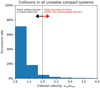 |
Fig. G.1 Histogram of the collision velocity, vcoll, for giant impacts occurring in all the 109 000 unstable compact systems. vcoll is expressed in units of the mutual escape velocity of the colliding bodies, vesc (Equation 2). We find that only 8% of collision occur at vcoll > 2vesc, for which our simplifying assumption that all debris produced by giant impacts are reaccreted by the target can artificially lower the mantle stripping efficiency (Section 2.2.3). Our results are therefore robust against this assumption. |
Appendix H Occurrence rate of compact systems for scenario T6
We estimate the occurrence rate of the compact systems in scenario T6 over the entire catalog of compact systems (thus, including both the compact systems from scenarios T6 and N0) as
 (H.1)
where N is the number of compact systems and f indicates the instability rate that we estimated for the compact systems. We use the latter to correct for those systems that are no longer compact because they went unstable in the past. For the scenario T6, Table F.1 yields NT6 = 12, NN0 = 90, fT6 = 0.5, and fN0 = 0.23. This translates to ηsys = 14%, revealing that the compact systems in scenario T6 are relatively rare among the whole observed set of compact systems.
(H.1)
where N is the number of compact systems and f indicates the instability rate that we estimated for the compact systems. We use the latter to correct for those systems that are no longer compact because they went unstable in the past. For the scenario T6, Table F.1 yields NT6 = 12, NN0 = 90, fT6 = 0.5, and fN0 = 0.23. This translates to ηsys = 14%, revealing that the compact systems in scenario T6 are relatively rare among the whole observed set of compact systems.
References
- Adibekyan, V., Dorn, C., Sousa, S. G., et al. 2021, Science, 374, 330 [NASA ADS] [CrossRef] [Google Scholar]
- Aguichine, A., Mousis, O., Devouard, B., & Ronnet, T. 2020, ApJ, 901, 97 [NASA ADS] [CrossRef] [Google Scholar]
- Allibert, L., Siebert, J., Hyodo, R., et al. 2025, Icarus, 429, 116385 [Google Scholar]
- Anderson, W. W., & Ahrens, T. J. 1994, J. Geophys. Res., 99, 4273 [NASA ADS] [CrossRef] [Google Scholar]
- Asphaug, E. 2010, Chem. Erde/Geochemistry, 70, 199 [NASA ADS] [Google Scholar]
- Asphaug, E., & Reufer, A. 2014, Nat. Geosci., 7, 564 [NASA ADS] [CrossRef] [Google Scholar]
- Ballard, S. 2019, Astron. J., 157, 113 [Google Scholar]
- Batygin, K. 2015, MNRAS, 451, 2589 [NASA ADS] [CrossRef] [Google Scholar]
- Boekholt, T., & Portegies Zwart, S. 2015, Computat. Astrophys. Cosmol., 2, 2 [NASA ADS] [CrossRef] [Google Scholar]
- Cambioni, S. 2025, Can metal-rich worlds form by giant impacts? (Supplementary Dataset) [Google Scholar]
- Cambioni, S., Asphaug, E., Emsenhuber, A., et al. 2019, ApJ, 875, 40 [NASA ADS] [CrossRef] [Google Scholar]
- Cambioni, S., Jacobson, S. A., Emsenhuber, A., et al. 2021, Planet. Sci. J., 2, 93 [CrossRef] [Google Scholar]
- Chambers, J. E. 2013, Icarus, 224, 43 [CrossRef] [Google Scholar]
- Connolly, J. A. D. 2009, Geochem. Geophys. Geosyst., 10, Q10014 [Google Scholar]
- Denman, T. R., Leinhardt, Z. M., & Carter, P. J. 2022, MNRAS, 513, 1680 [Google Scholar]
- Ebel, D. S., & Stewart, S. T. 2018, in Mercury. The View after MESSENGER, eds. S. C. Solomon, L. R. Nittler, & B. J. Anderson, 497 [CrossRef] [Google Scholar]
- Elkins-Tanton, L. T., Asphaug, E., Bell, J. F., et al. 2022, Space Sci. Rev., 218, 17 [NASA ADS] [CrossRef] [Google Scholar]
- Emsenhuber, A., Cambioni, S., Asphaug, E., et al. 2020, ApJ, 891, 6 [NASA ADS] [CrossRef] [Google Scholar]
- Emsenhuber, A., Asphaug, E., Cambioni, S., et al. 2024, Planet. Sci. J., 5, 59 [NASA ADS] [CrossRef] [Google Scholar]
- Essack, Z., Shporer, A., Burt, J. A., et al. 2023, AJ, 165, 47 [NASA ADS] [CrossRef] [Google Scholar]
- Esteves, L., Izidoro, A., Bitsch, B., et al. 2022, MNRAS, 509, 2856 [Google Scholar]
- Faber, J. A., Rasio, F. A., & Willems, B. 2005, Icarus, 175, 248 [NASA ADS] [CrossRef] [Google Scholar]
- Gabriel, T. S. J., & Cambioni, S. 2023, Annu. Rev. Earth Planet. Sci., 51, 671 [CrossRef] [Google Scholar]
- Gilbert, G. K. 1893, The Moon’s Face. A Study of the Origin of its Features (Philosophical Society of Washington) [Google Scholar]
- Gladman, B., & Coffey, J. 2009, Meteor. Planet. Sci., 44, 285 [Google Scholar]
- Goldberg, M., & Batygin, K. 2022, Astron. J., 163, 201 [Google Scholar]
- Goldreich, P., & Schlichting, H. E. 2014, Astron. J., 147, 32 [Google Scholar]
- Hadden, S., & Lithwick, Y. 2014, ApJ, 787, 80 [Google Scholar]
- Hadden, S., & Lithwick, Y. 2017, AJ, 154, 5 [Google Scholar]
- Hadden, S., & Lithwick, Y. 2018, AJ, 156, 95 [NASA ADS] [CrossRef] [Google Scholar]
- Hara, N. C., & Ford, E. B. 2023, Annu. Rev. Statist. Appl., 10, 623 [CrossRef] [Google Scholar]
- Hinkel, N. R., Timmes, F. X., Young, P. A., Pagano, M. D., & Turnbull, M. C. 2014, AJ, 148, 54 [NASA ADS] [CrossRef] [Google Scholar]
- Hinkel, N. R., Young, P. A., & Wheeler, Caleb H., I. 2022, AJ, 164, 256 [Google Scholar]
- Irving, J. C. E., Lekic’, V., Durán, C., et al. 2023, PNAS, 120, e2217090120 [Google Scholar]
- Izidoro, A., Ogihara, M., Raymond, S. N., et al. 2017, MNRAS, 470, 1750 [Google Scholar]
- Izidoro, A., Bitsch, B., Raymond, S. N., et al. 2021, A&A, 650, A152 [EDP Sciences] [Google Scholar]
- Johansen, A., & Dorn, C. 2022, A&A, 662, A19 [NASA ADS] [CrossRef] [EDP Sciences] [Google Scholar]
- Johnson, J. A., Petigura, E. A., Fulton, B. J., et al. 2017, AJ, 154, 108 [Google Scholar]
- Kenyon, S. J., & Bromley, B. C. 2006, AJ, 131, 1837 [Google Scholar]
- Kingma, D. P., & Ba, J. 2014, arXiv e-prints [arXiv:1412.6980] [Google Scholar]
- Lin, Z., Cambioni, S., & Seager, S. 2025, ApJ, 978, L41 [Google Scholar]
- Luo, H., Dorn, C., & Deng, J. 2024, Nat. Astron., 8, 1399 [Google Scholar]
- Luque, R., & Pallé, E. 2022, Science, 377, 1211 [NASA ADS] [CrossRef] [Google Scholar]
- MacDonald, M. G., Ragozzine, D., Fabrycky, D. C., et al. 2016, AJ, 152, 105 [Google Scholar]
- Marcus, R. A., Stewart, S. T., Sasselov, D., & Hernquist, L. 2009, ApJ, 700, L118 [CrossRef] [Google Scholar]
- Matsumoto, Y., & Ogihara, M. 2020, ApJ, 893, 43 [Google Scholar]
- McDonough, W. 2003, Treatise Geochem., 2, 568 [NASA ADS] [Google Scholar]
- Mishra, L., Alibert, Y., Leleu, A., et al. 2021, A&A, 656, A74 [NASA ADS] [CrossRef] [EDP Sciences] [Google Scholar]
- Mocquet, A., Grasset, O., & Sotin, C. 2014, Philos. Trans. Roy. Soc. Lond. Ser. A, 372, 20130164 [Google Scholar]
- Movshovitz, N., Nimmo, F., Korycansky, D. G., Asphaug, E., & Owen, J. M. 2016, Icarus, 275, 85 [Google Scholar]
- Mulders, G. D., Mordasini, C., Pascucci, I., et al. 2019, ApJ, 887, 157 [NASA ADS] [CrossRef] [Google Scholar]
- Murray, C. D., & Dermott, S. F. 2000, Solar System Dynamics (Cambridge, UK: Cambridge University Press) [Google Scholar]
- Naponiello, L., Mancini, L., Sozzetti, A., et al. 2023, Nature, 622, 255 [NASA ADS] [CrossRef] [Google Scholar]
- Nittler, L. R., Chabot, N. L., Grove, T. L., & Peplowski, P. N. 2018, in Mercury. The View after MESSENGER, eds. S. C. Solomon, L. R. Nittler, & B. J. Anderson, 30 [CrossRef] [Google Scholar]
- O’Brien, D. P., Morbidelli, A., & Levison, H. F. 2006, Icarus, 184, 39 [CrossRef] [Google Scholar]
- Otegi, J. F., Bouchy, F., & Helled, R. 2020, A&A, 634, A43 [NASA ADS] [CrossRef] [EDP Sciences] [Google Scholar]
- Owen, J. E. 2019, Annu. Rev. Earth Planet. Sci., 47, 67 [CrossRef] [Google Scholar]
- Palme, H., & O’Neill, H. S. C. 2003, Treatise Geochem., 2, 568 [NASA ADS] [Google Scholar]
- Parc, L., Bouchy, F., Venturini, J., Dorn, C., & Helled, R. 2024, A&A, 688, A59 [NASA ADS] [CrossRef] [EDP Sciences] [Google Scholar]
- Poon, S. T. S., Nelson, R. P., Jacobson, S. A., & Morbidelli, A. 2020, MNRAS, 491, 5595 [Google Scholar]
- Pu, B., & Wu, Y. 2015, ApJ, 807, 44 [Google Scholar]
- Reinhardt, C., Meier, T., Stadel, J. G., Otegi, J. F., & Helled, R. 2022, MNRAS, 517, 3132 [NASA ADS] [CrossRef] [Google Scholar]
- Rodríguez Martínez, R., Gaudi, B. S., Schulze, J. G., et al. 2023, Astron. J., 165, 97 [Google Scholar]
- Scora, J., Valencia, D., Morbidelli, A., & Jacobson, S. 2020, MNRAS, 493, 4910 [CrossRef] [Google Scholar]
- Scora, J., Valencia, D., Morbidelli, A., & Jacobson, S. 2022, ApJ, 940, 144 [Google Scholar]
- Shoemaker, E. M. 1962, in Physics and Astronomy of the Moon, ed. Z. Kopal (New York: Academic Press), 283 [Google Scholar]
- Steffen, J. H. 2016, MNRAS, 457, 4384 [NASA ADS] [CrossRef] [Google Scholar]
- Tamayo, D., Cranmer, M., Hadden, S., et al. 2020, PNAS, 117, 18194 [CrossRef] [PubMed] [Google Scholar]
- Unterborn, C. T., Desch, S. J., Haldemann, J., et al. 2023, ApJ, 944, 42 [Google Scholar]
- Villar, S., Yao, W., Hogg, D. W., Blum-Smith, B., & Dumitrascu, B. 2023, J. Mach. Learn. Res., 24, 1 [Google Scholar]
- Volk, K., & Gladman, B. 2015, ApJ, 806, L26 [Google Scholar]
- Volk, K., & Malhotra, R. 2020, AJ, 160, 98 [Google Scholar]
- Volk, K., & Malhotra, R. 2024, AJ, 167, 271 [Google Scholar]
- Weiss, L. M., Millholland, S. C., Petigura, E. A., et al. 2023, ASP Conference Series, 534, 863 [Google Scholar]
- Yee, S. W., Tamayo, D., Hadden, S., & Winn, J. N. 2021, AJ, 162, 55 [Google Scholar]
- Zeng, L., Jacobsen, S. B., Hyung, E., et al. 2021, ApJ, 923, 247 [NASA ADS] [CrossRef] [Google Scholar]
- Zhu, W., & Dong, S. 2021, Annu. Rev. Astron. Astrophys., 59, 291 [CrossRef] [Google Scholar]
All Tables
All Figures
|
Fig. 1 Formation theory for the observed high-density exoplanets. (a) Super-Earths are predicted to complete their formation through giant impacts whose energies are too low to strip their rocky mantles and form metal-rich planets (Scora et al. 2020, 2022; Poon et al. 2020; Esteves et al. 2022; Goldberg & Batygin 2022). (b) After their formation ceases, super-Earths can remain on closely spaced orbits typical of observed compact systems (Weiss et al. 2023) and can experience instabilities over timescales comparable to the main-sequence lifetime of their host stars (Volk & Gladman 2015; Pu & Wu 2015; Tamayo et al. 2020; Volk & Malhotra 2020). (c) If a compact system becomes unstable, super-Earths can experience a second stage of giant impacts that are more energetic than those that occurred during their formation (Volk & Gladman 2015). These late giant impacts may erode the silicate mantles of the super-Earths to form metal-rich, high-density planets. (d) The post-instability planetary systems may have a metal-rich world with density akin to the measured densities of observed high-density exoplanets (Table 1). Colors indicate different planetary compositions: orange is metal-rich, blue indicates planets with a terrestrial composition (that is, differentiated in an iron core and a rocky mantle with core-mass fraction ∼30 wt.%). |
| In the text | |
|
Fig. 2 Abundance of iron and rock-forming elements in the galactic neighborhood, selected planets, and meteorites. The green data points are the iron-to-silicon (Fe/Si) molar ratio versus magnesium-to-silicon (Mg/Si) molar ratio of stars with planets in the Hypatia catalog by Hinkel et al. (2014), along with the 68% (1σ), 95% (2σ) and 99.7% (3σ) isocontours, and the (Fe/Si, Mg/Si) of the CI carbonaceous chondrites, Earth, Mercury, and some of the high-density exoplanets in Table 1. The Fe/Si and Mg/Si values of the high-density exoplanets and Mercury are unknown. Here we assume that these planets have a Mg/Si equal to that of CI chondrites (the high-density nature of these planets does not change if other Mg/Si values are assumed). We then derive the bulk Fe/Si of planets from estimates of their core-mass fraction, Z, based on the measured masses and radii. We convert Z into Fe/Mg versus Si/Mg using Equation (13) from Unterborn et al. (2023), assuming that all the iron of the planet is in the core and that the mantle is composed of SiO2 and MgO. This plot is similar to Figure 7 from Unterborn et al. (2023), but here we plot only stars whose abundances [Fe/H], [Mg/H], and [Si/H] are known with uncertainties smaller than 30% and convert these values to molar ratios using the method by Hinkel et al. (2022). |
| In the text | |
|
Fig. 3 N-body evolution of the semimajor axis, a, of the super-Earths in the compact system Kepler-402 as a function of time, t. The values of a of the planets are initialized to their current (observed) value. The solid curves indicate the semimajor axes. The envelopes are the periapses and apoapses of the orbits. Upon instability, planet b merges with planet c and planet d merges with planet e by giant impacts. No planet becomes metal rich in this simulation, but a different outcome is possible for different initial eccentricities and mean longitudes. |
| In the text | |
|
Fig. 4 Flowchart of the statistical model of orbital instability. For details on each step, see Section 2.2.2. The symbols MT and MP indicate the masses of the target and projectile in the collisions, respectively. The symbols ZT and ZP indicate the core-mass fractions of the target and projectile of the collisions, respectively. The distributions from which the relative impact velocity, v∞ (in units of Keplerian velocity, vk) and impact angle, θ, are sampled are shown in Figure B.1c, d. |
| In the text | |
|
Fig. 5 Results from our orbital instability model for different model assumptions. Mass, M, as a function of radius, R, of the simulated planets surviving an orbital instability for the different model assumptions described in Section 2.3.1. The final planets are deemed metal-rich remnants (colored symbols) and non-metal-rich remnants (gray symbols) based on the high-density threshold of Equation (3). The black data points correspond to the observed high-density exoplanets listed in Table 1, with one standard deviation uncertainty bars; planet Mercury is plotted for comparison. The side plots are the Kernel Density Estimates (KDEs) of the radius (top) and mass (left) of the observed high-density planets (black curve) and the simulated metal-rich giant-impact remnants (colored curves). The model KDEs are weighted according to the probability of detection of the simulated metal-rich worlds by transit surveys, to mimic observational bias typical of exoplanetary surveys (Section 2.4). |
| In the text | |
|
Fig. 6 Hit-and-run collision between two super-Earths forming a metal-rich planet. Panels a through f: snapshots of a SPH simulation of a giant impact (times after collision listed at lower right each panel) from the dataset by Emsenhuber et al. (2024). The target body has mass MT = 2.5 M⊕ and core-mass fraction ZT = 0.30; particles composing the mantle and core of the target are colored in blue and red, respectively. The projectile has mass MP = 1 M⊕ and core-mass fraction ZP = 0.16; particles composing the mantle and core of the projectile are colored in purple and orange, respectively. The collision velocity is vcoll = 2.54 vesc and the impact angle is θ = 15° [see definitions in panel (a)]. Note scale bars at lower left. The projectile’s mantle is accreted by the target, while the projectile’s core escapes as a metal-rich planet. For an animation of this SPH simulation, see online Movie S1. |
| In the text | |
|
Fig. 7 Comparison of giant impacts among atmosphereless super-Earths to collisions involving atmosphere-rich targets. (a) Density of the surviving hit-and-run projectile, ρS, as a function of vcoll. The value of ρS is plotted in units of |
| In the text | |
|
Fig. 8 Likelihood that mantle-stripping giant impacts occur as a function of size of the colliding bodies. (a) Cumulative distribution of the radii, R, of the simulated metal-rich planets compared to that of the corresponding randomly eroded population generated as described in Section 3.3. (b) Same as panel a, but for planetary masses, M. (c) Fraction of initial super-Earths in unstable compact systems that evolve into metal-rich planets (i.e., probability of mantle stripping) as a function of their initial size, R0. (d) Fraction of compact systems that experienced instability (i.e., probability of system instability) as a function of the median initial planetary size, |
| In the text | |
|
Fig. 9 Implications of our results for the formation of metal-rich worlds. (a) Probability pGI that a late orbital instability forms metal-rich worlds as large and massive as the observed high-density exoplanets. The probability is computed as described in Section 2.4 and the planets are listed along the x-axis in order of increasing size. (b) Occurrence rate of the modeled metal-rich giant-impact remnants, ηMR, binned as a function of planetary radius, R. ηMR is computed as the fraction of the metal-rich worlds in the post-instability planetary population; the vertical bars indicate one standard deviation uncertainties computed across all simulation scenarios described in Table F.1. While most of the observed high-density exoplanets are too large to be metal-rich giant-impact remnants, sub-Earth-sized metal-rich worlds formed during a late orbital instabilities should be instead relatively common in the local galaxy but are likely too small to be detected by current exoplanetary surveys. |
| In the text | |
|
Fig. A.1 Effect of the radial-velocity bias on the detection of terrestrial planets. Left-bottom axes: Percent of terrestrial exoplanets detected, NR, as a function of the detection limit of RV signals, Kth, for different values of the orbital period P of the 100 terrestrial exoplanets in the model catalog. Right-top axes: Probability Density Function (PDF) of the RV signals of the observed terrestrial exoplanets in Dataset S1. |
| In the text | |
|
Fig. B.1 Input probability distributions for the orbital statistical model. a) Distribution of initial planets’ radius, R0, in the precursor compact systems whose properties are listed in Dataset S3. b) Distribution of initial planets’ mass, M0, in the compact systems (Dataset S3). c) Distribution of the relative impact velocity in units of Keplerian velocity, v∞/vk, assumed in the statistical model of Section 2.2.2. d) Distribution of the impact angle, θ assumed for the collision model in Section 2.2.2. The different curves are for the nominal case (N0) and the robustness tests (T1–T6). |
| In the text | |
|
Fig. C.1 Training history and performance of the optimal neural networks composing the giant-impact model. Panels a–g: Mean squared error (MSE) between y(x) predicted by the neural networks gi(i = 1,...,7) and the corresponding SPH outcome, t(x), as a function of the training epochs. The inset plots show the correlation with index R between y(x) and t(x) for the testing set. The complete training report (including the suboptimal neural networks) is in the Dataset S2. |
| In the text | |
|
Fig. D.1 Radius, R, as a function of semimajor axis, a, of planets in the planetary systems where high-density exoplanets have been observed. The data points are color coded by their masses, M (in units of M⊕). We plot only planets for which the radius and masses are known with sufficient precision to enable compositional estimates, i.e., σR/R <0.3 and σM/M <0.3. We distinguish between terrestrial planets (symbols with black edges) and volatile-rich planets (symbols with red edges) based on whether their R is greater or smaller than 2 R⊕, respectively (see Section 2.1.2). Most of the known planets in the systems with high-density exoplanets are predominantly made of rock and iron, with no large volatile envelopes. |
| In the text | |
|
Fig. E.1 Histograms of the period ratios of planets in compact systems. We distinguish between compact systems that are stable and likely to become unstable within the next 10–100 Myr following the procedure outlined in Section 2.2.2 (red and blue histograms, respectively). In the stable systems, we find that 30% of the planetary pairs are within 0.1 Pj+1/Pj of mean-motion resonances (7%, 15%, 4%, and 5% have period ratios 3:2, 2:1, 3:1, and 4:1 respectively). In the systems that we predict to be unstable, we find that 50% of the planetary pairs are within 0.1 Pj+1/Pj of mean-motion resonances (28%, 16%, 3%, and 2% have period ratios 3:2, 2:1, 3:1, and 4:1 respectively). Overall, this translates in 37% of the planetary pairs in the compact systems being within 0.1 Pj+1/Pj of the 3:2, 2:1, 3:1, and 4:1 mean-motion resonances. System-wise, 20% of the stable systems have planets in near–mean-motion resonances, while 70% of the unstable systems have planets in near–mean-motion resonances. |
| In the text | |
|
Fig. G.1 Histogram of the collision velocity, vcoll, for giant impacts occurring in all the 109 000 unstable compact systems. vcoll is expressed in units of the mutual escape velocity of the colliding bodies, vesc (Equation 2). We find that only 8% of collision occur at vcoll > 2vesc, for which our simplifying assumption that all debris produced by giant impacts are reaccreted by the target can artificially lower the mantle stripping efficiency (Section 2.2.3). Our results are therefore robust against this assumption. |
| In the text | |
Current usage metrics show cumulative count of Article Views (full-text article views including HTML views, PDF and ePub downloads, according to the available data) and Abstracts Views on Vision4Press platform.
Data correspond to usage on the plateform after 2015. The current usage metrics is available 48-96 hours after online publication and is updated daily on week days.
Initial download of the metrics may take a while.