| Issue |
A&A
Volume 695, March 2025
|
|
|---|---|---|
| Article Number | A215 | |
| Number of page(s) | 11 | |
| Section | Cosmology (including clusters of galaxies) | |
| DOI | https://doi.org/10.1051/0004-6361/202453203 | |
| Published online | 20 March 2025 | |
Limits and challenges of the detection of cluster-scale diffuse radio emission at high redshift
The Massive and Distant Clusters of WISE Survey (MaDCoWS) in LoTSS-DR2
1
INAF – Istituto di Radioastronomia, Via P. Gobetti 101, 40129 Bologna, Italy
2
Hamburger Sternwarte, Universität Hamburg, Gojenbergsweg 112, 21029 Hamburg, Germany
3
Green Bank Observatory, PO Box 2, Green Bank, WV 24944, USA
4
Kapteyn Astronomical Institute, University of Groningen, Landleven 12, 9747 AD Groningen, The Netherlands
5
Université Côte d’Azur, Observatoire de la Côte d’Azur, CNRS, Laboratoire, Lagrange, France
6
Leiden Observatory, Leiden University, PO Box 9513, 2300 RA Leiden, The Netherlands
7
Max Planck Institute for Astrophysics, Karl-Schwarzschild-Str. 1, D-85741 Garching, Germany
8
Space Research Institute (IKI), Profsoyuznaya 84/32, Moscow 117997, Russia
9
Universitäts-Sternwarte, Fakultät für Physik, Ludwig-Maximilians-Universität München, Scheinerstr.1, 81679 München, Germany
10
Centre for Astrophysics Research, University of Hertfordshire, College Lane, Hatfield AL10 9AB, UK
11
ASTRON, Netherlands Institute for Radio Astronomy, Oude Hoogeveensedijk 4, 7991 PD Dwingeloo, The Netherlands
12
Kazan Federal University, Kremlevskaya Str. 18, 420008 Kazan, Russia
13
University of California, Davis, CA 95616, USA
⋆ Corresponding author; gabriella.digennaro@inaf.it
Received:
28
November
2024
Accepted:
26
February
2025
Diffuse radio emission in galaxy clusters is a tracer of ultra-relativistic particles and μG-level magnetic fields, and is thought to be triggered by cluster merger events. In the distant Universe (i.e. z > 0.6), such sources have been observed only in a handful of systems, and their study is important to understand the evolution of large-scale magnetic fields over the cosmic time. Previous studies of nine Planck clusters up to z ∼ 0.9 suggest a fast amplification of cluster-scale magnetic fields, at least up to half of the current Universe’s age, and steep spectrum cluster scale emission, in line with particle re-acceleration due to turbulence. In this paper, we investigate the presence of diffuse radio emission in a larger sample of galaxy clusters reaching even higher redshifts (i.e. z ≳ 1). We selected clusters from the Massive and Distant Clusters of WISE Survey (MaDCoWS) with richness λ15 > 40 covering the area of the second data release of the LOFAR Two-Meter Sky Survey (LoTSS-DR2) at 144 MHz. These selected clusters are in the redshift range 0.78 − 1.53 (with a median value of 1.05). We detect the possible presence of diffuse radio emission, with the largest linear sizes of 350 − 500 kpc, in five out of the 56 clusters in our sample. If this diffuse radio emission is due to a radio halo, these radio sources lie on or above the scatter of the Pν − M500 radio halo correlations (at 150 MHz and 1.4 GHz) found at z < 0.6, depending on the mass assumed. We also find that these radio sources are at the limit of the detection by LoTSS, and therefore deeper observations are important for future studies.
Key words: radiation mechanisms: non-thermal / galaxies: clusters: general / galaxies: clusters: intracluster medium / large-scale structure of Universe
© The Authors 2025
 Open Access article, published by EDP Sciences, under the terms of the Creative Commons Attribution License (https://creativecommons.org/licenses/by/4.0), which permits unrestricted use, distribution, and reproduction in any medium, provided the original work is properly cited.
This article is published in open access under the Subscribe to Open model. Subscribe to A&A to support open access publication.
1. Introduction
In the ΛCDM cosmology, galaxy clusters grow via accretion of matter along the filaments of the cosmic web, and via mergers with other clusters and groups of galaxies (Press & Schechter 1974; Springel et al. 2006). Mergers involving these large-scale structures are the most energetic events in the Universe, releasing up to 1064 erg into the intracluster medium (ICM) within a cluster crossing time (i.e. ∼1 Gyr; Markevitch et al. 1999). These events affect the dynamics of the cluster galaxies (e.g. Golovich et al. 2019) and their properties (Stroe et al. 2017), and trigger turbulence and shocks (Markevitch & Vikhlinin 2007), with most of the energy eventually transferred to the ICM. Turbulence and shocks are thought to play an important role in (re-)accelerating particles up to relativistic energies (Lorentz factor γL ≫ 103) and in amplifying magnetic fields up to a few μG (Brunetti & Jones 2014; Carilli & Taylor 2002). Extended, cluster-centric, non-thermal radiation in the form of radio halos is observed in a large number of merging clusters (van Weeren et al. 2019; Botteon et al. 2022), especially at low radio frequencies (ν ≲ 100 MHz) due to their steep-spectra1. The halos are proposed to be generated via stochastic Fermi-II particle re-acceleration mechanisms due to turbulence (e.g. Brunetti et al. 2001; Petrosian 2001; Brunetti & Lazarian 2007, 2016). An additional, although sub-dominant (Adam et al. 2021), contribution to the radio halo emission could be provided by proton-proton collisions, which generate secondary electrons (Brunetti & Lazarian 2011; Pinzke et al. 2017; Brunetti et al. 2017). Since the turbulent energy budget is set by the cluster masses (Cassano & Brunetti 2005), more massive merging clusters are likely to host more powerful radio halos. Less powerful radio halos are also expected to have steeper spectral indices (i.e. α ≲ −1.5, see also Pasini et al. 2024). These properties have been observed by correlations in the halo power-mass diagram (Cuciti et al. 2021, 2023) and with ultra-steep spectrum sources (e.g. Brunetti et al. 2008).
Merger-induced turbulence associated with radio halos is thought to drive a small-scale dynamo, which amplifies magnetic fields after several eddy turnover times (i.e. several Gyr; Beresnyak & Miniati 2016). Estimates of cluster magnetic fields in the local Universe come from Faraday Rotation Measures, source depolarisation, inverse Compton (IC) upper limits, and equipartition arguments (Govoni & Feretti 2004; Bonafede et al. 2010; Osinga et al. 2022). These techniques agree in setting an average magnetic field level of a few μG, with a decreasing radial profile (Bonafede et al. 2010). These values have been found to remain roughly constant up to z ∼ 0.9, at least in massive systems, implying fast magnetic amplification during the formation of the first large-scale structures in the Universe (Di Gennaro et al. 2021a,b). The presence of diffuse radio emission on the Mpc scale was also recently reported in an extremely distant cluster, at z = 1.23 (i.e. ACT-CLJ0329.2-2330; Sikhosana et al. 2024). The origin of the “seeds” of cluster magnetic fields remains unclear, and it is still unknown whether they have a primordial (i.e. generated during the first phases of the Universe) or an astrophysical (i.e. injected by galactic winds, active galactic nuclei, and/or starbursts) origin (Subramanian et al. 2006; Tjemsland et al. 2023). Although numerical simulations suggest that a small-scale dynamo erases this information (Dolag et al. 1999; Cho 2014; Donnert et al. 2018; Domínguez-Fernández et al. 2019), observing synchrotron emission in distant galaxy clusters still provides constraints on the mechanisms of magnetic amplification and particle acceleration. Particle re-acceleration mechanisms predict a low occurrence fraction of these high-z radio sources (Cassano et al. 2023) and steep spectral index (i.e. α ≲ −1.5) because of the stronger losses due to the IC effect on the emitting particles.
In this paper, we investigate diffuse radio emission in a large sample of distant (i.e. z > 0.7) galaxy clusters selected from the Massive and Distant Clusters of Wise Survey (MaDCoWS; Gonzalez et al. 2019) using data from the second data release of the LOw Frequency Array (LOFAR; van Haarlem et al. 2013) Two-Meter Sky Survey (LoTSS-DR2; Shimwell et al. 2022). The combination of these two surveys represents a unique opportunity to study the cosmic evolution of the cluster-scale synchrotron emission, as MaDCoWS collects more than 2000 clusters at high redshift (z ≥ 0.7) and LoTSS-DR2 currently provides the most sensitive (100 μJy beam−1 at 6″ resolution) low-frequency (∼150 MHz) large survey. The manuscript is organised as follows: In Section 2 we define the sample selection; in Section 3 we describe the observations and the data calibration and imaging; results are presented in Section 4, and discussed in Section 5; finally, a summary is presented in Section 6. Throughout the paper, we assume a standard ΛCDM cosmology, with H0 = 70 km s−1 Mpc−1, Ωm = 0.3 and ΩΛ = 0.7.
2. Sample and cluster selection criteria
The Massive and Distant Clusters of WISE Survey (MaDCoWS; Gonzalez et al. 2019) is a catalogue of galaxy clusters in the redshift range 0.70 ≲ z ≲ 1.75, based upon Wide-field Infrared Survey Explorer (WISE; Wright et al. 2010) observations and complemented with data from the Panoramic Survey Telescope and Rapid Response System (PanSTARRS; Chambers et al. 2016) at Dec > −30° and from the SuperCOSMOS Sky Survey (Hambly et al. 2001) at Dec < −30°. From the WISE-PanSTARSS region, 1676 of the 2433 galaxy clusters detected by the survey have a photometric redshift (z) and a cluster richness (λ15; here, λ15 corresponds to the excess number density of galaxies selected by Spitzer color cuts as possible cluster members with a brightness cut-off of 15 μJy; see Gonzalez et al. 2019). Subsequent studies on the full MaDCoWS sample have attempted to calibrate the mass-richness relation. Particularly, comparisons with the Sunyaev-Zeldovich (SZ; Sunyaev & Zeldovich 1972) measurements using the Combined Array for mm-wave Astronomy (CARMA; Brodwin et al. 2015), the Atacama Compact Array (ACA; Di Mascolo et al. 2020), the MUSTANG2 camera on the Green Bank Telescope (Dicker et al. 2020), and the Atacama Cosmology Telescope (ACT; Orlowski-Scherer et al. 2021) have revealed that these clusters are in the M = 0.1 − 6 × 10¹⁴ M⊙ mass range, depending on the scaling relation used (Dicker et al. 2020).
In the LoTSS sky area with the best sensitivity, that is Dec ≥ 20°, the total number of clusters in MaDCoWs is 588. In this paper, we decided to focus on objects within the LoTSS-DR2 area (Shimwell et al. 2022) with a richness λ15 > 40, resulting in a final number of 64 clusters (see Fig. 1). The richness threshold of 40 was chosen in order to include the most massive clusters in the MaDCoWS sample, while also still retaining a large sample of clusters (Fig. 2). The final sample spans a wide photometric redshift range2, that is 0.78 ≤ z ≤ 1.53 (median ⟨zLoTSS⟩∼1.05), and richness, that is 40 < λ15 < 74 (see Table A.1 in Appendix A for the selected sample). This work thus extends the redshift and mass limits of our previously published work using the Planck PSZ2 catalogue (i.e. M500 = 4 − 8 × 10¹⁴ M⊙ and 0.6 ≤ z ≤ 0.9, Di Gennaro et al. 2021a).
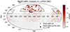 |
Fig. 1. Distribution of the MaDCoWS clusters in the PanSTARRS region (small dots), colour-coded based on their redshift. The grey area shows the sky region excluded because of the LoTSS sensitivity and sky coverage (i.e. Dec ≤ 20°). Large circles show the positions of the clusters in LoTSS-DR2 (see black outlines; Shimwell et al. 2022) with a richness λ15 > 40. |
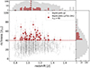 |
Fig. 2. Redshift-richness distribution of all the MaDCoWS clusters (small grey dots). The red, filled circles display the clusters in our sample (i.e. with λ15 > 40, see dashed line). The histograms on the top and on the right show their distribution in comparison with the full MaDCoWS sample. Dashed grey and red lines in the top-panel histogram show the median redshift of the two distributions (⟨zall⟩∼1.06 and ⟨zLoTSS⟩∼1.05, respectively). |
3. LOFAR data reduction and imaging
We have made use of the products of the LoTSS second data release (DR2). Therefore, we refer to Shimwell et al. (2022) for a detailed description of the radio data reduction. We applied the standard calibration pipeline, which corrects for direction-independent (prefactor; van Weeren et al. 2016; Williams et al. 2016; de Gasperin et al. 2019) and direction-dependent (ddf-pipeline, which includes killMS and DDFacet; Tasse 2014; Smirnov & Tasse 2015; Tasse et al. 2018, 2021) effects, and performs self-calibration of the entire field of view. To refine the solutions near the target, we also applied the “extraction & recalibration” strategy described by van Weeren et al. (2021). This procedure takes into account the local direction-dependent effects, by using the products of the pipeline, subtracting from the uv-plane all the sources outside a square region that includes the cluster (typically ∼0.3 − 0.9 deg2), and performing additional rounds of phase and amplitude self-calibration. At the end of the calibration, we assumed conservative residual uncertainties on the relative amplitude calibration of f = 0.15 (Shimwell et al. 2022). We also employed flux-scale alignment due to the uncertainties in the LOFAR beam modeling during the calibration, as described by Botteon et al. (2022) and Hoang et al. (2022). All the images and flux densities reported in the manuscript have these corrections applied.
Final, deep imaging was made using WSClean v2.10 (Offringa et al. 2014; Offringa & Smirnov 2017), with Briggs (Briggs 1995) weighting and robust=-0.5, and using multiscale deconvolution with scales of [1, 4, 8, 16]×pixelscale (pixelscale = 1.5″) and channelsout=6. An inner uv-cut at 80λ was applied to exclude the contribution of the Galactic emission. We produced images at different resolutions, tapering the uv-plane at 25 kpc, 50 kpc, and 100 kpc (see Appendix A, Fig. A.1). Additional higher-resolution images were created with robust=-1.25. To emphasise the possible presence of diffuse emission, we removed the contribution of compact sources: first we created a clean model only including compact sources (i.e. compact-only image), by excluding data below the uv-range corresponding to linear sizes ≥400 kpc (e.g. the typical size of radio halos; see van Weeren et al. 2019) at the cluster’s redshift. Then we subtracted this model and re-image the data, at different resolutions (i.e. without tapering, and with a taper of 25 kpc, 50 kpc, and 100 kpc; see Appendix A). For all the images, the final reference frequency is 144 MHz.
4. Results
We inspected the full-resolution, compact-only and low-resolution source-subtracted images by eye in order to investigate the presence of diffuse radio emission, similarly to what has been done by Botteon et al. (2022). A visual inspection was also made to exclude bad-quality data, that is, those affected by artefacts or poor calibration. We excluded from our final sample those clusters with a map noise that is greater than twice the nominal LoTSS value (with σrms,LoTSS = 100 μJy beam−1). These systems are: MOO J0907+2908 (σrms = 239 μJy beam−1), MOO J1110+6838 (σrms = 531 μJy beam−1), MOO J1135+3256 (σrms = 278 μJy beam−1), MOO J1336+4622 (σrms = 108 μJy beam−1) and MOO J1616+6053 (σrms = 474 μJy beam−1). Despite a favourable noise level (σrms = 64 μJy beam−1), MOO J1319+5519 was also excluded because it is located nearby a bright compact radio source that creates strong artefacts and therefore prevents any detection of diffuse radio emission. For similar reasons, we excluded MOO J1248+6723 and MOO J1506+5137, which are close to extended lower-redshift radio galaxies. In particular, the radio galaxy on the line of sight of MOO J1506+5137 (z = 0.611 at RAJ2000 = 15h06m12.81s and DecJ2000 = +51° 37′73″, Aguado et al. 2019) was extensively studied at radio frequencies using LOFAR, the Karl Jansky Very Large Array (VLA), and the Robert C. Byrd Green Bank Telescope (GBT) observations by Moravec et al. (2020). After excluding these eight clusters, the map noise in our sample ranges between 54 − 162 μJy beam−1, with a median value of 98 μJy beam−1 (see Fig. 3 and Appendix A).
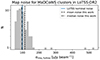 |
Fig. 3. Distribution of the map noise of the MaDCoWS clusters in LoTSS-DR2. The blue, solid line shows the nominal map noise from LoTSS, while the dot-dashed and dashed lines represent the median and mean values, respectively, for the 144 MHz cluster images in this work. |
We found that about 80% (44/56) of the clusters in the sample host at least one radio source (i.e. radio galaxy or extended diffuse radio source) at 144 MHz. Among these, we detect diffuse radio emission in the source-subtracted images with taper=100kpc covering the 0.5R500 region3 in five systems (see Fig. 4), namely MOO J0123+2545 (hereafter MOOJ0123, zspec = 1.229), MOO J1231+6533 (hereafter MOOJ1231, z = 0.99), MOO J1246+4642 (hereafter MOOJ1246, z = 0.90), MOO J1420+3150 (hereafter MOOJ1420, z = 1.34), and MOO J2354+3507 (hereafter MOOJ2354, z = 0.97). These radio sources have largest linear size (LLS) of roughly 350–500 kpc at the clusters’ redshift (i.e. angular size of ∼1′). For two systems, namely MOOJ0123 and MOOJ1231, SZ CARMA observation at 30 GHz (Decker et al. 2019) are also available, and show that the extended radio emission sits on the ICM (see Fig. 5). We show the overlay with the grz Desi Legacy Survey DR10 in Appendix B (Fig. B.1).
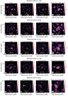 |
Fig. 4. LOFAR 144 MHz images of the MaDCoWS clusters with cluster-scale diffuse emission. The cluster name and redshift are stated at the top of each row. From left to right: full-resolution image; full resolution, compact only (i.e. after applying an inner uv-cut of 400 kpc; full-resolution source-subtracted image; same as previous panel, but with taper=100kpc. Yellow regions in the right panel of each row show the area where we measure the radio flux densities. Radio contours are displayed in white, solid lines, starting from 2.5σrms × [2, 4, 8, 16, 32] and negative contours at −2.5σrms are shown in white, dashed lines. The beam shape is shown at the bottom left corner of each panel. The dashed white circle shows the R500 kpc area, with the cross marking the MaDCoWS coordinates reported by Gonzalez et al. (2019) and, when available, the plus marking the peak of the CARMA SZ observation (Decker et al. 2019). |
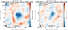 |
Fig. 5. CARMA 30 GHz observations (Decker et al. 2019) with radio source-subtracted LOFAR low-resolution contours of the available MaDCoWS clusters in LoTSS-DR2. The different beam sizes are shown the on the bottom left corner of each panel, with the solid grey corresponding to LoTSS-DR2 and open white to the CARMA 30 GHz data. The colour map represents the SZ variation in units of signal-to-noise, therefore negative values reveal the presence of the cluster (with the centre marked by the white ‘plus’; Decker et al. 2019). The black circle places the R500 area given the SZ coordinates, and the white cross provides the MaDCoWS centre (Gonzalez et al. 2019). The cluster mass, R500 and redshift from the CARMA observations are indicated in the upper left corner of each panel. |
4.1. Flux density measurements
We measure the flux density of the extended radio emission by integrating over the 2.5σrms radio contours from the source-subtracted image with taper=100kpc (S144MHz, sub). The total uncertainty for the flux density measurements is given by

where σrms is the map noise, and Nbeam is the number of beams covering the diffuse radio emission. The term σsub2 describes the goodness of the subtraction from the visibilities, and is equal to ∑iNbeams, i σrms2, namely the sum over all the i sources that were subtracted within the cluster region.
The source subtraction in the uv-plane can be imperfect. This is due to the presence of foreground radio galaxies with angular sizes similar to the cluster (which for this reason are excluded from the model of the subtracted sources), or because the source components are not entirely included in the model. In such cases, we exclude the extended emission of the radio galaxy from the source-subtracted flux density and/or manually subtract the residual flux density from those sources (S144 MHz, RG). The residual flux of the radio galaxies was estimated by comparing the emission from the full-resolution and compact-only images, following the 1σrms radio contours of the sources within the cluster region in the latter map. The final flux density on the diffuse emission is therefore defined as:
with the sum ∑iS144 MHz, RGi over all the ith-subtracted sources and ΔS144 MHz, RG calculated similarly to Eq. (1), but with σsub2 = 0.
Below, we describe the flux density measurements for each candidate cluster with extended diffuse radio emission, which are summarised in Table 1.
Flux densities of the cluster-scale diffuse radio emission at 144 MHz. Radio powers are calculated assuming a spectral index α = −1.5 ± 0.3 (Di Gennaro et al. 2021a,b).
4.1.1. MOOJ0123
This cluster shows extended radio emission in the full-resolution images, both in the original and source-subtracted images (see first row in Fig. 4). This emission is enhanced in the low-resolution image (i.e. taper=100kpc, corresponding to a resolution of ∼18″ × 15″). From this map, we measure a flux density of S144 MHz, sub = 2.5 ± 0.6 mJy within the area covering the 2.5σrms level (with σrms = 150 μJy beam−1, see the yellow region in the last column in Fig. 4). From this measured flux density, we additionally removed the residual contribution of the point sources visible in the compact-only image, that is ∑S144 MHz, RG = 0.4 ± 0.2 mJy. The final flux density for the diffuse radio emission in MOOJ0123 is S144 MHz, diff = 2.1 ± 0.6 mJy.
4.1.2. MOOJ1231
Hints of diffuse radio emission for this cluster are only visible in the source-subtracted taper=100kpc image (corresponding to a resolution of 19″ × 16″) at the 2.5σrms level, with σrms = 82 μJy beam−1 (see the second row in Fig. 4). However, the image is still contaminated by residual compact sources, which were excluded from the area of the diffuse radio emission (see yellow region in the last column). We measure a flux density of S144 MHz, sub = 1.3 ± 0.3 mJy, from which we additionally subtract ∑S144 MHz, RG = 0.3 ± 0.1 mJy of residual flux from a radio galaxy, leading to S144 MHz, diff = 1.0 ± 0.3 mJy.
4.1.3. MOOJ1246
Hints of extended diffuse radio emission for this cluster are visible in the full-resolution image, south of two compact sources (see the third row in Fig. 4). These two compact sources are not fully removed in the source subtraction process, we therefore exclude them from the area of the extended diffuse emission at low resolution (i.e. 26″ × 17″, with σrms = 340 μJy beam−1; see yellow region in the last column in Fig. 4). Here, we measure S144 MHz, sub = 1.7 ± 0.6 mJy and ∑S144 MHz, RG = 0.4 ± 0.2 mJy, and thus S144 MHz, diff = 1.3 ± 0.6 mJy.
4.1.4. MOOJ1420
The diffuse radio emission in the cluster is clearly visible in the source-subtracted taper=100kpc image (corresponding to a resolution of ∼18″ × 16″; see fourth row in Fig. 4). We measure a flux density within the 2.5σrms area (with σrms = 160 μJy beam−1, see yellow region in the last column in Fig. 4) of S144 MHz, sub = 3.1 ± 0.8 mJy. We estimate a residual flux density from the compact sources of ∑S144 MHz, RG = 1.3 ± 0.5 mJy. This corresponds to a flux density of the diffuse component of S144 MHz, diff = 1.8 ± 0.8 mJy.
4.1.5. MOOJ2354
The radio emission in the cluster in the full-resolution image is dominated by an extended radio galaxy, although we observe hints of faint diffuse radio emission south of it (see fifth row in Fig. 4). Hence, we define the area of the extended diffuse emission in the source-subtracted taper=100kpc image (corresponding to a resolution of 18″ × 15″) excluding the region covered by the radio galaxy (see the yellow region the last column in Fig. 4). We measure S144 MHz, sub = 1.6 ± 0.8 mJy.
4.2. Radio power estimation
For all the aforementioned clusters, we calculated the k-corrected radio luminosities at frequencies ν = 150 MHz and ν = 1.4 GHz, in order to compare to literature values (Cassano et al. 2013; Cuciti et al. 2021, 2023), as follows:
![$$ \begin{aligned} P_\nu = \frac{4\pi \,D_L(z)^2}{(1+z)^{\alpha +1}} \, \left(\frac{\nu }{\mathrm{144\,MHz}} \right)^{\alpha }S_{\rm 144\,MHz} \quad [\mathrm{W\,Hz}^{-1}]\,, \end{aligned} $$](/articles/aa/full_html/2025/03/aa53203-24/aa53203-24-eq3.gif)
where S144 MHz is the flux density of the diffuse emission measured at 144 MHz, α is the spectral index of the diffuse emission, DL is the luminosity distance at the redshift z, and the factor (1 + z)−(α + 1) is the k-correction. Since we do not have information on the spectral index for the clusters in the presented work, following Di Gennaro et al. (2021a,b) we assume α = −1.5 ± 0.3. Uncertainties in the radio luminosities are obtained with 150 Monte-Carlo simulations, which include both the uncertainties associated with the flux densities and the spectral indices. The flux densities at 144 MHz and the radio luminosities at 150 MHz and 1.4 GHz are listed in Table 1.
4.3. Upper limits
For 51 galaxy clusters in our sample, we did not detect extended diffuse radio emission in the cluster volume, and hence only upper limits can be provided. Following Bruno et al. (2023), we calculate our upper limits as:
Here, σrms is the source-subtracted taper=100kpc map noise, and Nbeam is the number of beams covering the radio halo region. We define the area of the halo region equal to 3re, being re = 75 kpc the cluster e-folding radius, which corresponds to a physical size comparable to those we detect in our sample (i.e 450 kpc, ∼1′). Given the low number of beams covering the radio halo region (Nbeam ≲ 10), we adopt the best-fit parameters of m = 0.5 and q = 0.155 (Di Gennaro et al. 2021b; Bruno et al. 2023). As for the detected diffuse extended emission, we then derive radio luminosities of the upper limits at 150 MHz and 1.4 GHz assuming a spectral index of α = −1.5 ± 0.3 in Eq. (3) (see Appendix C, Fig, C.1).
4.4. Cluster mass
In order to investigate the properties of the extended diffuse radio emission in the MaDCoWS clusters, and to have a comparison with diffuse sources at lower redshifts, it is crucial to have an estimate of the cluster mass. Literature mass measurements are available only for MOOJ0123 and MOOJ1231, through CARMA 30 GHz observations (Decker et al. 2019), being M500 = (3.9 ± 0.8)×1014 M⊙ and M500 = (4.7 ± 1.1)×1014 M⊙, respectively (Table 2). For the other clusters, we can make use of scaling relations via optical-IR, SZ and X-ray observations.
Mass estimation of the clusters in our sample with diffuse radio emission.
4.4.1. Mass-richness relation
Masses for the MaDCoWS clusters can be retrieved from their galaxy richness (Brodwin et al. 2015; Gonzalez et al. 2019; Di Mascolo et al. 2020; Dicker et al. 2020; Orlowski-Scherer et al. 2021), according to the relation:
In this work we assume the relation found by Orlowski-Scherer et al. (2021), where an extensive calibration of the relation was performed by analysing the MaDCoWS-selected clusters on forced-photometry estimates from ACT observations and resulting in  and
and  , with an intrinsic scatter
  . We report the resulting cluster mass in Table 2, including the uncertainties due to the scatter of the relation (numbers in brackets in the third column).
Comparing the only two mass estimates from CARMA 30 GHz observations with the mass we would obtain using the M500 − λ15 scaling relation, we find the corresponding ones from the scaling relation are a factor of ∼2 lower, although consistent within 1σ errorbar including the scatter of the relation. This difference is probably associated with the different assumptions regarding the integrated SZ signal to mass scaling relation adopted by Decker et al. (2019) and Orlowski-Scherer et al. (2021).
4.4.2. Masses from eROSITA observations
The MaDCoWS clusters in the LoTSS-DR2 samples are covered in the SRG/eROSITA all-sky survey (Sunyaev et al. 2021; Predehl et al. 2021). We, therefore, can use X-ray data to estimate their masses. For z ∼ 1 clusters the X-ray flux turns out to be a useful mass proxy (e.g. Churazov et al. 2015). The X-ray flux was estimated from the 0.4–2.3 keV count rate within a circle with radius R = 2′ centred at the cluster position (see Table A.1), and using a wider ring from 6′ to 20′ to estimate the local X- ray background signal. For the latter, bright point and extended sources, with the 0.5–2 keV flux above 10−13 erg s−1 cm−2 are detected and masked, following the strategy described by Churazov et al. (2021) and Khabibullin et al. (2023). The variance in the background flux within the source aperture was estimated in a model-independent way, selecting 24 regions of the same size within a 30′ circle centred on the cluster candidate. The extracted count rates within the source apertures are corrected for the expected background contributions and finally converted to the 0.5–2 keV flux, FX, using a constant factor, which weakly depends on the cluster temperature (see, e.g. Fig. B1 in Lyskova et al. 2023, for the temperature dependence of emissivity in the 0.3–2.3 keV band). Uncertainties on the flux are set by the photon count statistics (Poisson noise, σstat) and the average background variance contribution (σvar = 1.5 × 10⁻¹⁴ erg s−1 cm−2), that is  .
.
The cluster mass is then estimated via the following relation (Churazov et al. 2015):
where the factor z0.5 is expected to work well in the redshift range ∼0.7 − 1.5 when scaling relations from Vikhlinin et al. (2009) are used, while η encapsulates factors related to the method of flux estimation, the sample selection function, and the definition of the mass. We use η = 0.86 found for a subset of ACT clusters with z > 0.7 from Orlowski-Scherer et al. (2021) sample using ACT_MASS value as the mass proxy (for details, we refer to Lyskova et al. in prep.). The retrieved masses are reported in Table 2. From these eROSITA observations, we found a good agreement (within 1σ) with the masses obtained from the Orlowski-Scherer et al. (2021) mass-richness relation except for MOOJ1231, for which the X-ray mass is similar to the CARMA 30 GHz one (Decker et al. 2019). This could suggest a more complicated morphology of this cluster than the others in the sample.
5. Discussion
Given the radio power of the diffuse radio emission in our sample (Sect. 4.2) and the estimated masses of the host clusters (Sect. 4.4), we can place these systems in the canonical radio power-mass diagram for a comparison with the diffuse radio emission at lower redshift (see Fig. 6; Cassano et al. 2013; Cuciti et al. 2023). In this context, we interpreted our detections as candidate radio halo emission, due to their central location with respect to the distribution of the cluster galaxies and taking into account the uncertainties on the radio galaxies subtraction and the lack of a clear overlay with the thermal emission of the ICM. Following the same criteria as in Botteon et al. (2022), we do not separate candidate mini-halos from giant halos based on the size of the radio emission in our targets. Specifically, in Fig. 6 we show all the Planck clusters with a detected diffuse radio emission in LoTSS (left column; Di Gennaro et al. 2021a; Botteon et al. 2022) and their corresponding radio power at 1.4 GHz (right column) using a spectral index of α = −1.3 for the clusters at z < 0.6 and α = −1.5 for the clusters at z > 0.6 (Di Gennaro et al. 2021a). For these lower-redshift clusters, the existence of such a correlation has been extensively proved, both at 150 MHz and 1.4 GHz. In particular, the recent analysis of the Planck clusters in the LoTSS-DR2 area has confirmed the presence of a correlation between cluster mass and radio power over a wide mass and redshift range (i.e. M500 ∼ 3 − 10 × 1014 M⊙ and z ∼ 0.02 − 0.6), although the analysis was focused only on clusters above the 50% completeness level of the Planck clusters (Cuciti et al. 2023, see dashed line in the left panels in Fig. 6). The parameters (i.e. slope and normalisation) of the correlation at 150 MHz and 1.4 GHz were found to be in line with previous literature studies based on smaller samples at the same frequency (Cassano et al. 2013, see dashed line in the right panels in Fig. 6). The existence of such a correlation is interpreted as the amount of energy injected by turbulence into the intracluster medium which then powers particle re-acceleration and the small-scale dynamo for the magnetic amplification. Therefore, the most massive clusters are expected to host the most powerful radio halos (Cassano & Brunetti 2005). The implication is that the properties of the extended radio emission lying on this correlation, such as the average magnetic fields (⟨B⟩) and the turbulent energy (ηt, i.e. the fraction of the PdV work done by the sub-clusters falling into the main cluster) can be assumed to be similar in clusters regardless their mass and redshift. Recent work has shown a good agreement between theoretical models and observations, at least up to z < 0.4 (Cassano et al. 2023). Clusters with lower average magnetic fields would be placed below the correlation, including its scatter (see Fig. 3a of Di Gennaro et al. 2021a). High-redshift clusters hosting extended diffuse radio emission are hence expected to populate this region of the Pν − M500 diagram, as magnetic fields are thought to evolve from weak (primordial or astrophysical) seeds through compression and turbulence (Vazza et al. 2018).
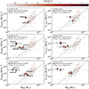 |
Fig. 6. Radio power versus mass diagrams (150 MHz, left column; 1.4 GHz, right column). Small shaded circles are from the literature at lower-redshifts (Di Gennaro et al. 2021a; Botteon et al. 2022), while stars display the detection from the MaDCoWS clusters in LoTSS-DR2 presented in this work. All markers are colour-coded according to their redshifts. We also display the Pν − M500 correlations found by Cuciti et al. (2023) and Cassano et al. (2013), at 150 MHz (left panels) and 1.4 GHz (right panles) respectively. Top row: masses from CARMA 30 GHz observations (Decker et al. 2019). Middle row: masses from the richness-mass scale relation calibrated with ACT clusters (Orlowski-Scherer et al. 2021, OS+21); solid errorbars reflect the uncertainties on the slope of the scale relation, while the dashed errorbars define the uncertainties associated with the scatter of the scale relation. Bottom row: masses from eROSITA observation. |
Three of the five clusters in the final sample – namely MOOJ1231, MOOJ1246 and MOOJ2354 – fall within the scatter of the Pν − M500 distributions of the lower redshift systems. This is regardless of whether we use the mass obtained from the M500 − λ15 or the M500 − FX scaling relations, although the former tends towards lower values. On the other hand, the only cluster among these three systems with also CARMA observations, MOOJ1231, has a mass that is more consistent with the M500 − FX scale relation (i.e. 4.7 ± 1.1 × 10¹⁴ M⊙ and  , respectively; see Table 2). The two highest redshift clusters, instead, – namely MOOJ0123 and MOOJ1420 – are well above the radio power-mass correlation, using the masses obtained from the mass-richness scaling relation or the ones from the X-ray flux from eROSITA observations. However, similarly to MOOJ1231, the CARMA observation for MOOJ0123 points to a higher mass, that is ∼2 times higher than those from those obtained from the scale relations. Assuming this latter mass, this cluster would also lie within the scatter of the correlation found by Cuciti et al. (2023). It is worth noting that the CARMA high frequency observations (i.e. 30 GHz) are characterised by poor resolution (i.e. 40″) and low sensitivity, combined with interferometric filtering, and single-frequency data.
If we assume that the masses estimated from the scaling relations are reliable, considering the high redshifts of these clusters – and therefore the stronger Inverse Compton energy losses (i.e. dE/dt ∝ (1 + z)4) –, the location of these systems above the Pν − M500 correlation is quite surprising. Following the reasoning by Di Gennaro et al. (2021a), at high redshift it is expected that the flux of turbulent energy (ρvt3/Linj, where ρ is the gas density, and vt and Linj are the turbulent velocity and injection scale, respectively) is about 3 times higher than that dissipated at lower redshift (z ∼ 0.2) because of the larger impact velocities and virial densities of merging clusters. This translates to an average magnetic field level in clusters at z ∼ 0.7 that would be similar to that in the low-redshift ones, that is ∼few μG, if we measured similar radio power of the diffuse radio emission. Assuming the amount of flux of turbulent energy remains constant between z ∼ 0.7 and z ∼ 1 with respect to the low-redshift regime (and that ηt is redshift-independent), the over-luminosity of 2 orders of magnitude we see in our sample suggests an average magnetic field level that is up to one order of magnitude higher than at low redshift.
This result would pose challenges in the understanding the evolution of magnetic fields in galaxy clusters over the cosmic time. The only other cluster known so far to clearly host a radio halo at z > 1 is ACT-CL J0329.2-2330 (z = 1.23; Sikhosana et al. 2024). Moreover, a putative claim for extended radio emission was also made for SPT-CL J2106-584 (z = 1.13; Di Mascolo et al. 2021), although with the data in hand it was not possible to unambiguously separate the contribution of the of individual cluster galaxies. These systems are both placed on the P1.4 GHz − M500 correlation, therefore suggesting ∼μG-level magnetic fields, but, in contrast to those from our sample, they are extremely massive ( and
and  , respectively). For these cases, it is plausible that the formation of the systems started earlier in the cosmic evolution of the Universe and, therefore, they would amplify their magnetic fields up to the ∼μG level earlier.
We finally note that from the full sample of the MaDCoWS clusters in LoTSS-DR2, we retrieve a detection rate for diffuse radio emission of ∼9% (i.e. 5 candidate extended radio emission over 56 clusters), in the redshift range 0.78–1.53. This is much smaller than the ∼50% value previously found by Di Gennaro et al. (2021a), for the z = 0.6 − 0.9 redshift range and much larger cluster masses (MSZ, 500 ∼ 4 − 8 × 10¹⁴ M⊙). Although this is a simplistic comparison, which does not take into account the different sample selection (i.e. SZ versus optical), the decreasing detection rate with the redshift is not unexpected because of the largest energy losses due to IC effects on the relativistic particles (dE/dt ∝ (1 + z)4) and because of the low masses of our MaDCoWS clusters, as also highlighted by theoretical models (Cassano et al. 2023).
5.1. Caveats
The comparison with the low-redshift samples in the Pν − M500 diagram is strongly affected by the uncertainties in the mass estimation, and on the discrepancies among the targeted observations (with CARMA at 30 GHz, see Decker et al. 2019) and the values obtained through the scaling relations, both from the IR-selected richness and from the X-ray flux. This uncertainty reflects on the interpretation on the origin of the extended radio emission in these high-z clusters, where a difference of a factor of 2 in mass strongly shifts the position of the cluster with the respect to the correlation. This is clearly seen for MOOJ0123, which is located within the scatter of the correlation if the mass estimated by the CARMA observations is taken, while it is more than one order of magnitude more radio luminous assuming the mass obtained from the two scale relations. A reliable estimation of the cluster mass, for instance with the MUSTANG-2, at the Green Bank Telescope (GBT) at 90 GHz (Dicker et al. 2014), is therefore a crucial point for such studies. This is currently under investigation and is part of a forthcoming work.
Moreover, the radio luminosities are estimated by assuming a given spectral index (α = −1.5 ± 0.3) which is taken from limited literature studies at high redshift (Di Gennaro et al. 2021a,b). This, however, would only affect P1.4 GHz and would not justify the position of two orders of magnitude above the scatter of the clusters at low redshift for MOOJ0123 and MOOJ1420. Following Di Gennaro et al. (2021b), higher-frequency observations with the uGMRT could help to determine a more precise spectral index of this extended diffuse radio emission, while lower-frequency observations with LOFAR LBA would be limited by poorer resolution (i.e. 15″) and sensitivity (∼1 mJy beam−1; see de Gasperin et al. 2023).
Finally, we cannot completely exclude that part of the radio emission seen as extended in the cluster volume is actually due to blending of unresolved active galactic nuclei (AGN). To quantify this effect, we artificially masked all the observed radio galaxies in the full resolution source-subtracted images, and then successively smooth the data to lower resolutions (i.e. taper=100kpc). Using this method, the flux densities of the diffuse emission decrease of 25–40%. To better exploit the effect of the contamination of faint AGN in the full sample, observations with the International LOFAR Telescope (ILT) – whose antennas are located throughout Europe – are necessary to provide the necessary resolution (up to sub-arcsecond) to disentangle the two kinds of different radio emission.
5.2. Limits from LoTSS observations
As mentioned in Sect. 4.3, most of the clusters in the MaDCoWS sample in the LoTSS-DR2 area do not show radio emission on the Mpc scale. To investigate whether this is a limit due to the observations, we derived the minimum flux detectable by LoTSS observation as presented by Cassano et al. (2023):
![$$ \begin{aligned} S_{\rm 150\,MHz,lim}({ < }3\Theta _e,z)=4.44\times 10^{-3} \xi \, {\sigma _{\rm rms}} \left( \frac{\Theta _e(z)}{\Theta _{\rm beam}} \right) \quad [\mathrm{mJy}]. \end{aligned} $$](/articles/aa/full_html/2025/03/aa53203-24/aa53203-24-eq24.gif)
Here, σrms = 200 μJy beam−1 is the nominal map noise at low resolution (i.e. taper=100kpc) of a standard LoTSS observation of 8 hours4 (Shimwell et al. 2022), Θbeam is the observing resolution in arcsecond, Θe is the angular size of the e-folding radius re, being equal to 75 kpc (see Sect. 4.3). All the parameters described above are set to roughly describe the behaviour of the upper limits from our sample (Cassano et al. 2023). The minimum radio power detectable at 150 MHz was then calculated using Eq. (3), assuming different values for different spectral indices, i.e. α = [ − 1.0, −1.3, −1.5, −1.8].
In Fig. 7, we show the comparison of this theoretical limit and all the clusters in our sample. As expected, all the clusters with diffuse radio emission are above the P150 MHz, lim(z, α) curve, while the upper limits are all located on the theoretical limits. This means that at the high redshift (z > 0.8) and relatively low mass (M500 ≲ 4 × 10¹⁴ M⊙) of the MaDCoWS clusters, we are limited by the LoTSS sensitivity (Shimwell et al. 2022). In Appendix D, we show the comparison of the evolution of the detectable radio power with deeper observations (i.e. observing time 100 hours), reaching a noise level σrms = 55 μJy beam−1 at the same low resolution (that is Θbeam = 100 kpc, see Fig. D.1).
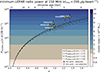 |
Fig. 7. Detection limit as a function of the redshift (z), as detectable by a standard LoTSS observation (Eq. (7)). Different lines show the dependence of the radio power on different spectral indices (solid, α = −1.5; dot-dashed, α = −1.0; dashed, α = −1.3; dotted, α = −1.8). The colour bar and the coloured bands refer to the mass that a galaxy cluster should have to lie exactly on the P150 MHz − M500 correlation found by Cuciti et al. (2023). Clusters from the MaDCoWS-LoTSS DR2 sample are also displayed (detections with golden stars, and non-detections with low-vertices triangles). |
We also show in colour shades the mass that a galaxy cluster should have to lie exactly on the P150 MHz − M500 correlation presented in Cuciti et al. (2023), i.e.:
with A = 1.1 ± 0.09 and B = 3.45 ± 0.44. Although we do not take into account the scatter of the correlation, this implies that at z = 0.8 and at z = 1.4 clusters with masses M500 ≳ 4 × 10¹⁴ M⊙ and M500 ≳ 6 × 10¹⁴ M⊙, respectively, could in principle be detectable to host extended radio emission and following the correlation. Clusters with such high masses are supposed to be rare, in the context of the ΛCDM cosmology, at such high redshift (Menanteau et al. 2012; Katz et al. 2013; Jee et al. 2014). At the same time, the comparison with expected cluster masses and the P150MHz, lim curve challenges the chances to populate the region below the correlation, where the high-z radio halos should lie, because of the expected lower magnetic field levels (Di Gennaro et al. 2021a). Deeper LOFAR observations (> 100 hours on target; see Tasse et al. 2021) could in principle help to detect lower-mass clusters (see Appendix D, Fig. D.1), but they are demanding, and therefore would be feasible only for a selected number of clusters and not for large surveys.
6. Summary and future analysis
In this paper, we have attempted for the first time to investigate the presence of extended and diffuse radio emission in a large sample of galaxy clusters selected at high redshift (i.e. z > 0.75). We have made use of the Massive and Distant Clusters of WISE Survey (MaDCoWS; Gonzalez et al. 2019), where we select clusters with richness λ15 > 40 which are in the second data release of the LOFAR Two-Meter Sky Survey (LoTSS-DR2).
The final sample collects 56 galaxy clusters with a median redshift ⟨zLoTSS⟩ = 1.05. Among these, only 5 systems show hints of diffuse radio emission on the cluster scale (i.e. a fraction of about 9%). All these candidate radio halos have integrated flux densities that correspond to radio powers that are above the P150 MHz − M500 and P1.4 GHz − M500 correlations at lower redshifts (Cuciti et al. 2023; Cassano et al. 2013, respectively). However, we stress that the mass values we report for the clusters in our sample are still very uncertain. Future targeted SZ observations with MUSTANG-2, at the Green Bank Telescope (GBT) at 90 GHz (Dicker et al. 2014), or near-IR observations, with the James Webb Space Telescope (JWST; Jakobsen et al. 2022; Böker et al. 2023) and the ESA-Euclid mission (Laureijs et al. 2011; Euclid Collaboration: Scaramella et al. 2022), would provide a more reliable estimation of the mass values.
We also investigated the limitations of our radio observations. Assuming a standard LoTSS setting (i.e. 8 hr on pointing) where a sensitivity of 200 μJy beam−1 at low resolution (Θbeam = 100 kpc) is reached, we are only able to detect the most powerful cluster-scale diffuse radio emission with radio powers at z > 0.8 (i.e. P150 MHZ > 1025 W Hz−1). If we assume an exact relation between the luminosity of the diffuse radio emission and the cluster mass according to Cuciti et al. (2023), this would imply that clusters with masses above 6 × 10¹⁴ M⊙ could be observed to host such extended diffuse radio sources. Additionally, we should keep in mind that the fraction of Planck clusters found to host a radio halo is only ∼30% (Botteon et al. 2022), averaged for a large range of redshift (z = 0.016 − 0.9, with a median of 0.280) and mass (MSZ,500 = 1.1 − 11.7 × 10¹⁴ M⊙, with a median of 4.9 × 10¹⁴ M⊙). This fraction is expected to decrease at higher redshift and, especially, for lower masses (Cassano et al. 2023).
All these findings pose a limitation on the detection of diffuse radio emission from samples of high-redshift clusters. However, the forthcoming large high-redshift surveys with a reliable estimation of the cluster mass – such as Euclid, where > 105 clusters are expected to be found up to z ∼ 2 – provide interesting systems to target with deep LOFAR HBA observations.
Data availability
Appendix to this manuscript is available on Zenodo (https://zenodo.org/records/14959262). The radio observations are available in the LOFAR Long Term Archive (LTA; https://lta.lofar.eu/). The data that support the plots within this paper and other findings of this study are available from the corresponding author upon reasonable request.
We estimated R500 from M500 obtained by the mass-richness scaling relation from Orlowski-Scherer et al. (2021), see Sect. 4.4.1.
Acknowledgments
We thank the referee for the suggestions which improved the quality of the manuscript. GDG and FdG acknowledge support from the ERC Consolidator Grant ULU 101086378. GDG and MB acknowledge funding by the DFG under Germany’s Excellence Strategy – EXC 2121 “Quantum Universe” – 390833306. MJH thanks the UK STFC for support [ST/V000624/1, ST/Y001249/1]. RJvW acknowledges support from the ERC Starting Grant ClusterWeb 804208. IK acknowledges support by the COMPLEX project from the European Research Council (ERC) under the European Union’s Horizon 2020 research and innovation program grant agreement ERC-2019-AdG 882679. LOFAR data products were provided by the LOFAR Surveys Key Science project (LSKSP; https://lofar-surveys.org/) and were derived from observations with the International LOFAR Telescope (ILT). LOFAR (van Haarlem et al. 2013) is the Low Frequency Array designed and constructed by ASTRON. It has observing, data processing, and data storage facilities in several countries, which are owned by various parties (each with their own funding sources), and which are collectively operated by the ILT foundation under a joint scientific policy. The ILT resources have benefited from the following recent major funding sources: CNRS-INSU, Observatoire de Paris and Université d’Orléans, France; BMBF, MIWF-NRW, MPG, Germany; Science Foundation Ireland (SFI), Department of Business, Enterprise and Innovation (DBEI), Ireland; NWO, The Netherlands; The Science and Technology Facilities Council, UK; Ministry of Science and Higher Education, Poland; The Istituto Nazionale di Astrofisica (INAF), Italy. This research made use of the Dutch national e-infrastructure with support of the SURF Cooperative (e-infra 180169) and the LOFAR e-infra group. The Jülich LOFAR Long Term Archive and the German LOFAR network are both coordinated and operated by the Jülich Supercomputing Centre (JSC), and computing resources on the supercomputer JUWELS at JSC were provided by the Gauss Centre for Supercomputing e.V. (grant CHTB00) through the John von Neumann Institute for Computing (NIC). This research made use of the University of Hertfordshire high-performance computing facility and the LOFAR-UK computing facility located at the University of Hertfordshire and supported by STFC [ST/P000096/1], and of the Italian LOFAR IT computing infrastructure supported and operated by INAF, and by the Physics Department of Turin university (under an agreement with Consorzio Interuniversitario per la Fisica Spaziale) at the C3S Supercomputing Centre, Italy. This work is based on observations with eROSITA telescope on board SRG space observatory. The SRG observatory was built by Roskosmos in the interests of the Russian Academy of Sciences represented by its Space Research Institute (IKI) in the framework of the Russian Federal Space Program, with the participation of the Deutsches Zentrum für Luftund Raumfahrt (DLR). The eROSITA X-ray telescope was built by a consortium of German Institutes led by MPE, and supported by DLR. The SRG spacecraft was designed, built, launched and is operated by the Lavochkin Association and its subcontractors. The science data are downlinked via the Deep Space Network Antennae in Bear Lakes, Ussurijsk, and Baikonur, funded by Roskosmos. The eROSITA data used in this work were converted to calibrated event lists using the eSASS software system developed by the German eROSITA Consortium and analysed using proprietary data reduction software developed by the Russian eROSITA Consortium. This research made use of APLpy, an open-source plotting package for Python (Robitaille & Bressert 2012), astropy, a community-developed core Python package for Astronomy (Astropy Collaboration 2013, 2018), matplotlib (Hunter 2007), and numpy (Harris et al. 2020).
References
- Adam, R., Goksu, H., Brown, S., Rudnick, L., & Ferrari, C. 2021, A&A, 648, A60 [NASA ADS] [CrossRef] [EDP Sciences] [Google Scholar]
- Aguado, D. S., Ahumada, R., Almeida, A., et al. 2019, ApJS, 240, 23 [Google Scholar]
- Astropy Collaboration (Robitaille, T. P., et al.) 2013, A&A, 558, A33 [NASA ADS] [CrossRef] [EDP Sciences] [Google Scholar]
- Astropy Collaboration (Price-Whelan, A. M., et al.) 2018, AJ, 156, 123 [Google Scholar]
- Beresnyak, A., & Miniati, F. 2016, ApJ, 817, 127 [NASA ADS] [CrossRef] [Google Scholar]
- Böker, T., Beck, T. L., Birkmann, S. M., et al. 2023, PASP, 135, 038001 [CrossRef] [Google Scholar]
- Bonafede, A., Feretti, L., Murgia, M., et al. 2010, A&A, 513, A30 [NASA ADS] [CrossRef] [EDP Sciences] [Google Scholar]
- Botteon, A., Shimwell, T. W., Cassano, R., et al. 2022, A&A, 660, A78 [NASA ADS] [CrossRef] [EDP Sciences] [Google Scholar]
- Briggs, D. S. 1995, Bull. Am. Astron. Soc., 27, 1444 [Google Scholar]
- Brodwin, M., Greer, C. H., Leitch, E. M., et al. 2015, ApJ, 806, 26 [Google Scholar]
- Brunetti, G., & Jones, T. W. 2014, Int. J. Mod. Phys. D, 23, 1430007 [Google Scholar]
- Brunetti, G., & Lazarian, A. 2007, MNRAS, 378, 245 [Google Scholar]
- Brunetti, G., & Lazarian, A. 2011, MNRAS, 410, 127 [Google Scholar]
- Brunetti, G., & Lazarian, A. 2016, MNRAS, 458, 2584 [Google Scholar]
- Brunetti, G., Setti, G., Feretti, L., & Giovannini, G. 2001, MNRAS, 320, 365 [Google Scholar]
- Brunetti, G., Giacintucci, S., Cassano, R., et al. 2008, Nature, 455, 944 [Google Scholar]
- Brunetti, G., Zimmer, S., & Zandanel, F. 2017, MNRAS, 472, 1506 [Google Scholar]
- Bruno, L., Brunetti, G., Botteon, A., et al. 2023, A&A, 672, A41 [NASA ADS] [CrossRef] [EDP Sciences] [Google Scholar]
- Carilli, C. L., & Taylor, G. B. 2002, ARA&A, 40, 319 [NASA ADS] [CrossRef] [Google Scholar]
- Cassano, R., & Brunetti, G. 2005, MNRAS, 357, 1313 [Google Scholar]
- Cassano, R., Ettori, S., Brunetti, G., et al. 2013, ApJ, 777, 141 [Google Scholar]
- Cassano, R., Cuciti, V., Brunetti, G., et al. 2023, A&A, 672, A43 [NASA ADS] [CrossRef] [EDP Sciences] [Google Scholar]
- Chambers, K. C., Magnier, E. A., Metcalfe, N., et al. 2016, ArXiv e-prints [arXiv:1612.05560] [Google Scholar]
- Cho, J. 2014, ApJ, 797, 133 [NASA ADS] [CrossRef] [Google Scholar]
- Churazov, E., Vikhlinin, A., & Sunyaev, R. 2015, MNRAS, 450, 1984 [CrossRef] [Google Scholar]
- Churazov, E., Khabibullin, I., Lyskova, N., Sunyaev, R., & Bykov, A. M. 2021, A&A, 651, A41 [NASA ADS] [CrossRef] [EDP Sciences] [Google Scholar]
- Cuciti, V., Cassano, R., Brunetti, G., et al. 2021, A&A, 647, A51 [EDP Sciences] [Google Scholar]
- Cuciti, V., Cassano, R., Sereno, M., et al. 2023, A&A, 680, A30 [NASA ADS] [CrossRef] [EDP Sciences] [Google Scholar]
- Decker, B., Brodwin, M., Abdulla, Z., et al. 2019, ApJ, 878, 72 [NASA ADS] [CrossRef] [Google Scholar]
- de Gasperin, F., Dijkema, T. J., Drabent, A., et al. 2019, A&A, 622, A5 [NASA ADS] [CrossRef] [EDP Sciences] [Google Scholar]
- de Gasperin, F., Edler, H. W., Williams, W. L., et al. 2023, A&A, 673, A165 [NASA ADS] [CrossRef] [EDP Sciences] [Google Scholar]
- Dicker, S. R., Ade, P. A. R., Aguirre, J., et al. 2014, in Millimeter, Submillimeter, and Far-Infrared Detectors and Instrumentation for Astronomy VII, eds. W. S. Holland, &J. Zmuidzinas, SPIE Conf. Ser., 9153, 91530J [NASA ADS] [CrossRef] [Google Scholar]
- Dicker, S. R., Romero, C. E., Di Mascolo, L., et al. 2020, ApJ, 902, 144 [NASA ADS] [CrossRef] [Google Scholar]
- Di Gennaro, G., van Weeren, R. J., Brunetti, G., et al. 2021a, Nat. Astron., 5, 268 [Google Scholar]
- Di Gennaro, G., van Weeren, R. J., Cassano, R., et al. 2021b, A&A, 654, A166 [NASA ADS] [CrossRef] [EDP Sciences] [Google Scholar]
- Di Mascolo, L., Mroczkowski, T., Churazov, E., et al. 2020, A&A, 638, A70 [NASA ADS] [CrossRef] [EDP Sciences] [Google Scholar]
- Di Mascolo, L., Mroczkowski, T., Perrott, Y., et al. 2021, A&A, 650, A153 [NASA ADS] [CrossRef] [EDP Sciences] [Google Scholar]
- Dolag, K., Bartelmann, M., & Lesch, H. 1999, A&A, 348, 351 [NASA ADS] [Google Scholar]
- Domínguez-Fernández, P., Vazza, F., Brüggen, M., & Brunetti, G. 2019, MNRAS, 486, 623 [Google Scholar]
- Donnert, J., Vazza, F., Brüggen, M., & ZuHone, J. 2018, Space Sci. Rev., 214, 122 [Google Scholar]
- Euclid Collaboration (Scaramella, R., et al.) 2022, A&A, 662, A112 [NASA ADS] [CrossRef] [EDP Sciences] [Google Scholar]
- Golovich, N., Dawson, W. A., Wittman, D. M., et al. 2019, ApJS, 240, 39 [NASA ADS] [CrossRef] [Google Scholar]
- Gonzalez, A. H., Gettings, D. P., Brodwin, M., et al. 2019, ApJS, 240, 33 [NASA ADS] [CrossRef] [Google Scholar]
- Govoni, F., & Feretti, L. 2004, Int. J. Mod. Phys. D, 13, 1549 [Google Scholar]
- Hambly, N. C., MacGillivray, H. T., Read, M. A., et al. 2001, MNRAS, 326, 1279 [NASA ADS] [CrossRef] [Google Scholar]
- Harris, C. R., Millman, K. J., van der Walt, S. J., et al. 2020, Nature, 585, 357 [NASA ADS] [CrossRef] [Google Scholar]
- Hoang, D. N., Brüggen, M., Botteon, A., et al. 2022, A&A, 665, A60 [NASA ADS] [CrossRef] [EDP Sciences] [Google Scholar]
- Hunter, J. D. 2007, Comput. Sci. Eng., 9, 90 [NASA ADS] [CrossRef] [Google Scholar]
- Jakobsen, P., Ferruit, P., Alves de Oliveira, C., et al. 2022, A&A, 661, A80 [NASA ADS] [CrossRef] [EDP Sciences] [Google Scholar]
- Jee, M. J., Hughes, J. P., Menanteau, F., et al. 2014, ApJ, 785, 20 [NASA ADS] [CrossRef] [Google Scholar]
- Katz, H., McGaugh, S., Teuben, P., & Angus, G. W. 2013, ApJ, 772, 10 [NASA ADS] [CrossRef] [Google Scholar]
- Khabibullin, I. I., Churazov, E. M., Bykov, A. M., Chugai, N. N., & Sunyaev, R. A. 2023, MNRAS, 521, 5536 [NASA ADS] [CrossRef] [Google Scholar]
- Laureijs, R., Amiaux, J., Arduini, S., et al. 2011, ArXiv e-prints [arXiv:1110.3193] [Google Scholar]
- Lyskova, N., Churazov, E., Khabibullin, I. I., et al. 2023, MNRAS, 525, 898 [NASA ADS] [CrossRef] [Google Scholar]
- Markevitch, M., & Vikhlinin, A. 2007, Phys. Rep., 443, 1 [Google Scholar]
- Markevitch, M., Sarazin, C. L., & Vikhlinin, A. 1999, ApJ, 521, 526 [Google Scholar]
- Menanteau, F., Hughes, J. P., Sifón, C., et al. 2012, ApJ, 748, 7 [NASA ADS] [CrossRef] [Google Scholar]
- Moravec, E., Gonzalez, A. H., Dicker, S., et al. 2020, ApJ, 898, 145 [Google Scholar]
- Offringa, A. R., & Smirnov, O. 2017, MNRAS, 471, 301 [Google Scholar]
- Offringa, A. R., McKinley, B., Hurley-Walker, N., et al. 2014, MNRAS, 444, 606 [Google Scholar]
- Orlowski-Scherer, J., Di Mascolo, L., Bhandarkar, T., et al. 2021, A&A, 653, A135 [NASA ADS] [CrossRef] [EDP Sciences] [Google Scholar]
- Osinga, E., van Weeren, R. J., Andrade-Santos, F., et al. 2022, A&A, 665, A71 [NASA ADS] [CrossRef] [EDP Sciences] [Google Scholar]
- Pasini, T., De Gasperin, F., Brüggen, M., et al. 2024, A&A, 689, A218 [NASA ADS] [CrossRef] [EDP Sciences] [Google Scholar]
- Petrosian, V. 2001, ApJ, 557, 560 [Google Scholar]
- Pinzke, A., Oh, S. P., & Pfrommer, C. 2017, MNRAS, 465, 4800 [Google Scholar]
- Predehl, P., Andritschke, R., Arefiev, V., et al. 2021, A&A, 647, A1 [EDP Sciences] [Google Scholar]
- Press, W. H., & Schechter, P. 1974, ApJ, 187, 425 [Google Scholar]
- Robitaille, T., & Bressert, E. 2012, Astrophysics Source Code Library [record ascl:1208.017] [Google Scholar]
- Shimwell, T. W., Hardcastle, M. J., Tasse, C., et al. 2022, A&A, 659, A1 [NASA ADS] [CrossRef] [EDP Sciences] [Google Scholar]
- Sikhosana, S. P., Hilton, M., Bernardi, G., et al. 2024, ArXiv e-prints [arXiv:2404.03944] [Google Scholar]
- Smirnov, O. M., & Tasse, C. 2015, MNRAS, 449, 2668 [Google Scholar]
- Springel, V., Frenk, C. S., & White, S. D. M. 2006, Nature, 440, 1137 [NASA ADS] [CrossRef] [Google Scholar]
- Stroe, A., Sobral, D., Paulino-Afonso, A., et al. 2017, MNRAS, 465, 2916 [NASA ADS] [CrossRef] [Google Scholar]
- Subramanian, K., Shukurov, A., & Haugen, N. E. L. 2006, MNRAS, 366, 1437 [CrossRef] [Google Scholar]
- Sunyaev, R. A., & Zeldovich, Y. B. 1972, Comm. Astrophys. Space Phys., 4, 173 [Google Scholar]
- Sunyaev, R., Arefiev, V., Babyshkin, V., et al. 2021, A&A, 656, A132 [NASA ADS] [CrossRef] [EDP Sciences] [Google Scholar]
- Tasse, C. 2014, A&A, 566, A127 [NASA ADS] [CrossRef] [EDP Sciences] [Google Scholar]
- Tasse, C., Hugo, B., Mirmont, M., et al. 2018, A&A, 611, A87 [NASA ADS] [CrossRef] [EDP Sciences] [Google Scholar]
- Tasse, C., Shimwell, T., Hardcastle, M. J., et al. 2021, A&A, 648, A1 [EDP Sciences] [Google Scholar]
- Tjemsland, J., Meyer, M., & Vazza, F. 2023, ArXiv e-prints [arXiv:2311.04273] [Google Scholar]
- van Haarlem, M. P., Wise, M. W., Gunst, A. W., et al. 2013, A&A, 556, A2 [NASA ADS] [CrossRef] [EDP Sciences] [Google Scholar]
- van Weeren, R. J., Brunetti, G., Brüggen, M., et al. 2016, ApJ, 818, 204 [Google Scholar]
- van Weeren, R. J., de Gasperin, F., Akamatsu, H., et al. 2019, Space Sci. Rev., 215, 16 [Google Scholar]
- van Weeren, R. J., Shimwell, T. W., Botteon, A., et al. 2021, A&A, 651, A115 [NASA ADS] [CrossRef] [EDP Sciences] [Google Scholar]
- Vazza, F., Brunetti, G., Brüggen, M., & Bonafede, A. 2018, MNRAS, 474, 1672 [NASA ADS] [CrossRef] [Google Scholar]
- Vikhlinin, A., Burenin, R. A., Ebeling, H., et al. 2009, ApJ, 692, 1033 [Google Scholar]
- Williams, W. L., van Weeren, R. J., Röttgering, H. J. A., et al. 2016, MNRAS, 460, 2385 [Google Scholar]
- Wright, E. L., Eisenhardt, P. R. M., Mainzer, A. K., et al. 2010, AJ, 140, 1868 [Google Scholar]
All Tables
Flux densities of the cluster-scale diffuse radio emission at 144 MHz. Radio powers are calculated assuming a spectral index α = −1.5 ± 0.3 (Di Gennaro et al. 2021a,b).
All Figures
|
Fig. 1. Distribution of the MaDCoWS clusters in the PanSTARRS region (small dots), colour-coded based on their redshift. The grey area shows the sky region excluded because of the LoTSS sensitivity and sky coverage (i.e. Dec ≤ 20°). Large circles show the positions of the clusters in LoTSS-DR2 (see black outlines; Shimwell et al. 2022) with a richness λ15 > 40. |
| In the text | |
|
Fig. 2. Redshift-richness distribution of all the MaDCoWS clusters (small grey dots). The red, filled circles display the clusters in our sample (i.e. with λ15 > 40, see dashed line). The histograms on the top and on the right show their distribution in comparison with the full MaDCoWS sample. Dashed grey and red lines in the top-panel histogram show the median redshift of the two distributions (⟨zall⟩∼1.06 and ⟨zLoTSS⟩∼1.05, respectively). |
| In the text | |
|
Fig. 3. Distribution of the map noise of the MaDCoWS clusters in LoTSS-DR2. The blue, solid line shows the nominal map noise from LoTSS, while the dot-dashed and dashed lines represent the median and mean values, respectively, for the 144 MHz cluster images in this work. |
| In the text | |
|
Fig. 4. LOFAR 144 MHz images of the MaDCoWS clusters with cluster-scale diffuse emission. The cluster name and redshift are stated at the top of each row. From left to right: full-resolution image; full resolution, compact only (i.e. after applying an inner uv-cut of 400 kpc; full-resolution source-subtracted image; same as previous panel, but with taper=100kpc. Yellow regions in the right panel of each row show the area where we measure the radio flux densities. Radio contours are displayed in white, solid lines, starting from 2.5σrms × [2, 4, 8, 16, 32] and negative contours at −2.5σrms are shown in white, dashed lines. The beam shape is shown at the bottom left corner of each panel. The dashed white circle shows the R500 kpc area, with the cross marking the MaDCoWS coordinates reported by Gonzalez et al. (2019) and, when available, the plus marking the peak of the CARMA SZ observation (Decker et al. 2019). |
| In the text | |
|
Fig. 5. CARMA 30 GHz observations (Decker et al. 2019) with radio source-subtracted LOFAR low-resolution contours of the available MaDCoWS clusters in LoTSS-DR2. The different beam sizes are shown the on the bottom left corner of each panel, with the solid grey corresponding to LoTSS-DR2 and open white to the CARMA 30 GHz data. The colour map represents the SZ variation in units of signal-to-noise, therefore negative values reveal the presence of the cluster (with the centre marked by the white ‘plus’; Decker et al. 2019). The black circle places the R500 area given the SZ coordinates, and the white cross provides the MaDCoWS centre (Gonzalez et al. 2019). The cluster mass, R500 and redshift from the CARMA observations are indicated in the upper left corner of each panel. |
| In the text | |
|
Fig. 6. Radio power versus mass diagrams (150 MHz, left column; 1.4 GHz, right column). Small shaded circles are from the literature at lower-redshifts (Di Gennaro et al. 2021a; Botteon et al. 2022), while stars display the detection from the MaDCoWS clusters in LoTSS-DR2 presented in this work. All markers are colour-coded according to their redshifts. We also display the Pν − M500 correlations found by Cuciti et al. (2023) and Cassano et al. (2013), at 150 MHz (left panels) and 1.4 GHz (right panles) respectively. Top row: masses from CARMA 30 GHz observations (Decker et al. 2019). Middle row: masses from the richness-mass scale relation calibrated with ACT clusters (Orlowski-Scherer et al. 2021, OS+21); solid errorbars reflect the uncertainties on the slope of the scale relation, while the dashed errorbars define the uncertainties associated with the scatter of the scale relation. Bottom row: masses from eROSITA observation. |
| In the text | |
|
Fig. 7. Detection limit as a function of the redshift (z), as detectable by a standard LoTSS observation (Eq. (7)). Different lines show the dependence of the radio power on different spectral indices (solid, α = −1.5; dot-dashed, α = −1.0; dashed, α = −1.3; dotted, α = −1.8). The colour bar and the coloured bands refer to the mass that a galaxy cluster should have to lie exactly on the P150 MHz − M500 correlation found by Cuciti et al. (2023). Clusters from the MaDCoWS-LoTSS DR2 sample are also displayed (detections with golden stars, and non-detections with low-vertices triangles). |
| In the text | |
Current usage metrics show cumulative count of Article Views (full-text article views including HTML views, PDF and ePub downloads, according to the available data) and Abstracts Views on Vision4Press platform.
Data correspond to usage on the plateform after 2015. The current usage metrics is available 48-96 hours after online publication and is updated daily on week days.
Initial download of the metrics may take a while.