| Issue |
A&A
Volume 695, March 2025
|
|
|---|---|---|
| Article Number | A36 | |
| Number of page(s) | 22 | |
| Section | Stellar atmospheres | |
| DOI | https://doi.org/10.1051/0004-6361/202452964 | |
| Published online | 03 March 2025 | |
MINCE
III. Detailed chemical analysis of the UVES sample★
1
ESO – European Southern Observatory,
Alonso de Cordova 3107,
Vitacura, Santiago,
Chile
2
GEPI, Observatoire de Paris, Université PSL, CNRS,
5 Place Jules Janssen,
92190
Meudon,
France
3
INAF – Osservatorio Astronomico di Trieste,
Via G.B. Tiepolo 11,
34143
Trieste,
Italy
4
Universidad Andres Bello, Facultad de Ciencias Exactas, Departamento de Físicas y Astronomía – Instituto de Astrofísica, Autopista Concepción-Talcahuano,
7100
Talcahuano,
Chile
5
Dipartimento di Fisica, Sezione di Astronomia, Università di Trieste,
Via G. B. Tiepolo 11,
34143
Trieste,
Italy
6
INFN, Sezione di Trieste,
Via A. Valerio 2,
34127
Trieste,
Italy
7
UPJV, Université de Picardie Jules Verne, Pôle Scientifique,
33 rue St Leu,
80039,
Amiens,
France
8
Institute for Applied Physics, Goethe University Frankfurt,
Max-von-Laue-Strasse 1,
60438
Frankfurt am Main,
Germany
9
Division of Astronomy and Space Physics, Department of Physics and Astronomy, Uppsala University,
Box 516,
75120
Uppsala,
Sweden
10
Institute of Theoretical Physics and Astronomy, Vilnius University,
Saulėtekio al. 3,
10257
Vilnius,
Lithuania
11
Dipartimento di Fisica e Astronomia “Augusto Righi”, Alma Mater Studiorum, Universitá di Bologna,
Via Gobetti 93/2,
40129
Bologna,
Italy
12
INAF – Osservatorio di Astrofisica e Scienza dello Spazio di Bologna,
Via Gobetti 93/3,
40129
Bologna,
Italy
13
INAF – Osservatorio Astrofisico di Arcetri,
Largo E. Fermi, 5,
50125,
Firenze,
Italy
★★ Corresponding author; This email address is being protected from spambots. You need JavaScript enabled to view it.
Received:
12
November
2024
Accepted:
17
January
2025
Abstract
Context. The Measuring at Intermediate Metallicity Neutron-Capture Elements (MINCE) project aims to provide high-quality neutron-capture abundances measurements for several hundred stars at an intermediate metallicity of −2.5 < [Fe/H] < −1.5. This project will shed light on the origin of the neutron-capture elements and the chemical enrichment of the Milky Way. Aims. The goal of this work is to chemically characterize the second sample of the MINCE project and compare the abundances with the galactic chemical evolution model at our disposal.
Methods. We performed a standard abundance analysis based on one-dimensional (1D) local thermodynamic equilibrium (LTE) model atmospheres based on high-resolution and high-signal-to-noise-ratio (S/N) spectra from Ultraviolet and Visual Echelle Spectrograph (UVES).
Results. We provide the kinematic classification (i.e., thin disk, thick disk, thin-to-thick disk, halo, Gaia Sausage Enceladus, Sequoia) of 99 stars and the atmospheric parameters for almost all stars. We derived the abundances for light elements (from Na to Zn) and neutron-capture elements (Rb, Sr, Y, Zr, Ba, La, Ce, Pr, Nd, Sm, and Eu) for a subsample of 32 stars in the metallicity range of −2.5 < [Fe/H] < −1.00. In the subsample of 32 stars, we identified eight active stars exhibiting (inverse) P-Cygni profile and one Li-rich star, CD 28-11039. We find a general agreement between the chemical abundances and the stochastic model computed for the chemical evolution of the Milky Way halo for elements Mg, Ca, Si, Ti, Sc, Mn, Co, Ni, Zn, Rb, Sr, Y, Zr, Ba, La, and Eu .
Conclusions. The MINCE project has already significantly increased the number of neutron-capture elements measurements in the intermediate metallicity range. The results from this sample are in perfect agreement with the previous MINCE sample. The good agreement between the chemical abundances and the chemical evolution model of the Galaxy supports the nucleosynthetic processes adopted to describe the origin of the n-capture elements.
Key words: nuclear reactions, nucleosynthesis, abundances / stars: abundances / stars: atmospheres / Galaxy: evolution / Galaxy: halo
This paper is based on data collected with the Very Large Telescope (VLT) at the European Southern Observatory (ESO) on Paranal, Chile (ESO Program ID: 105.20ML.001, 106.21PG.001).
© The Authors 2025
 Open Access article, published by EDP Sciences, under the terms of the Creative Commons Attribution License (https://creativecommons.org/licenses/by/4.0), which permits unrestricted use, distribution, and reproduction in any medium, provided the original work is properly cited.
This article is published in open access under the Subscribe to Open model. This email address is being protected from spambots. You need JavaScript enabled to view it. to support open access publication.
1 Introduction
One way to constrain the Galaxy’s formation and evolution is to carry out a detailed chemical analysis of its stellar populations. The main ingredients for this purpose are a complete census of the stellar populations hosted by the Galaxy and a deep investigation of the different nucleosynthesis processes. The goal of the Measuring at Intermediate Metallicity NeutronCapture Elements (MINCE, Cescutti et al. 2022) project is to fill in the chemical abundances of mildly metal-poor stars (−2.5 < [Fe/H] < −1.5).
The understanding of early Galactic neutrosynthesis processes and chemical evolution led to pursuits of increasingly metal-poor stars. This effort increased with the discovery of carbon-enhanced metal-poor (CEMP) stars (Sneden et al. 1994; Barbuy et al. 1997; Norris et al. 1997; Bonifacio et al. 1998; Hill et al. 2000) characterized by different neutron-capture (n- capture) element content (Cohen et al. 2003; Beers & Christlieb 2005; Hansen et al. 2012; Roederer et al. 2014; Yong et al. 2014). At the same time, the n-capture elements abundances in halo stars have been analyzed in several Galactic archaeology studies (see e.g., François et al. 2003, 2007, and references therein). As a result, the old giant stars with intermediate metallicity have been less examined by the scientific community.
The bulk of elements heavier than iron are produced through slow (s), rapid (r) or intermediate (i) neutron capture processes. The difference among these processes lie in the neutron density, which determines the probability of capturing a neutron before the radioactive beta decay (Burbidge et al. 1957). The s-process occurs in the inter-shell region of asymptotic giant branch (AGB) stars with low and intermediate mass (Gallino et al. 1998; Busso et al. 1999; Karakas & Lattanzio 2014). Both Supernovae and neutron star mergers have been proposed as sites hosting the r-process (Argast et al. 2004; Côté et al. 2018; Watson et al. 2019; Cavallo et al. 2021; Cowan et al. 2021). Despite several suggested sites, the site of the i-process remains an open question (Hampel et al. 2016, 2019; Denissenkov et al. 2017). For a recent review on the origin of the elements, we refer to Arcones & Thielemann (2023). Another puzzle concerning n- capture elements abundances is their large star-to-star scatter at low metallicities. Indeed, it has been shown that the dispersion in [n-capture/Fe] increases as metallicity decreases. This finding provides critical insights into the origin of n-capture elements (Hansen et al. 2014) and the processes of formation of the MW.
In summary, the measurement of n-capture elements in intermediate metallicity stars will allow us to increase our knowledge on the contribution from the different n-capture processes. Consequently, this will provide new insights into the origin of the heavy elements and their progenitor stars may be achieved. This will also shed light on the early interstellar medium (ISM) pollution process and its timescales (Côté et al. 2019), which are fundamental details that will contribute to improving the Galactic chemical evolution models. In this work, we present the chemical abundances of the second MINCE sample (hereafter, referred to as MINCE III) obtained for light elements (from Na to Zn) and n-capture elements (Rb, Sr, Y, Zr, Ba, La, Ce, Pr, Nd, Sm, Eu), along with a comparison to the chemical evolution model of the Galaxy.
2 Observations and data reduction
The MINCE project exploits several facilities around the world to collect high-quality data and provides precise atmospheric parameters and chemical abundances of stars at intermediate metallicity. In this paper, we present a sample of 99 stars observed with Ultraviolet and Visual Echelle Spectrograph (UVES, Dekker et al. 2000) at European Southern Observatory’s Very Large Telescope and second Unit Telescope of Paranal Observatory (Chile). The data were collected between September 2020 and August 2021. The instrument was set with two configurations: Dichroic#1, with blue and red arms centered at 346 nm and 580 nm, respectively, and Dichroic#2, with blue and red arms centered at 437 nm and 760 nm, respectively. The final dataset for each star covers the spectral range 304-945 nm. A slit width of 0.5 arcsec was used, providing a high resolving power of R ∼ 65 000 and R ∼ 75 000 in blue and red spectra, respectively. The data were reduced using the UVES pipeline (version 5.10.131 ). The final spectra are characterized by high signal-to-noise ratio (S/N), with mean values of 148 at 580 nm and 105 at 760 nm. The coordinates and the Gaia early Data- Release (eDR3, Gaia Collaboration 2021) magnitudes of the sample can be found in Table B.1 (available at the CDS).
2.1 Radial velocities
The Gaia Data-Release (DR3, Gaia Collaboration 2023) radial velocities (RV) of the targets used in this work are listed in Table B.1 (available at the CDS), when available. When the radial velocity was not available from Gaia DR3, it was estimated directly from our UVES spectrum (label b in the comment column of Table B.1).
These values were used to shift the observed spectra to the rest frame. However, in the case of six stars we did not find a good match between the synthetic and the observational spectra. For CD-28 10387, we found an RV difference of 7.49 km s−1. For this star, Gaia DR3 provides a RUWE value of 3.63, suggesting a possible binary nature. In the case of CD-29 15930 and CD-31 16658, we applied an additional shift of −4.99 km s−1and −7.49 km s−1, respectively. The final RV of CD-31 16922 differs from the Gaia one by 17.47 km s−1. It is interesting to note that Gaia estimates an error on the RV of about 9.08 km s−1 for this star. The largest shift corrections found are those corresponding to CD-44 12644 (−29.95 km s−1) and TYC 5422-1192-1 (19.97 km s−1).
Except for TYC 5422-1192-1, we do not detect the contribution of a companion in the spectra of the above mentioned stars. Thus, we can reasonably exclude the possibility that these stars are double-lined spectroscopic binary (SB2) and that the companion contributes to the spectrum to explain the disagreements with Gaia RV. It is, however, quite likely that these five stars are single lined spectroscopic binaries; the future release of Gaia epoch radial velocities will help to elucidate this issue. Taking into account the shift estimated, we corrected the Gaia RV and reported the final results in Table B.1 (label a in the comment column).
3 Analysis
3.1 Stellar parameters
Each derivation method for the stellar parameters leads to systematic errors in the estimation of chemical abundances. Since the MINCE project has at its disposal several spectra, a homogeneous way to derive the stellar parameters is required to present consistent analysis. For this reason, we obtained the atmospheric parameters as described in Cescutti et al. (2022).
Starting from the Gaia eDR3 (Gaia Collaboration 2021) photometry, we first obtained the dereddened G magnitude and GBP − GRP color of the targets. Extinction estimates were made for each target star according to the following scheme. The first step uses the extinction density maps presented by Vergely et al. (2022). For each star, the extinction density (in mag per pc) is integrated along the paths between the Sun and the star to provide the total extinction. Details of the maps can be found in Vergely et al. (2022). In brief, they were computed by inversion of about 40 million individual extinction measurements for stars with precise distances, mainly Gaia parallaxes. The inversion was regularised on the basis of a covariance kernel (or minimum cloud size) adapted to the volume density of the targets through a hierarchical scheme. In addition to the three maps presented in that work, for close targets, we also used an additionalunpublished map with a minimum kernel size of 5 pc (courtesy J.L. Vergely). The largest map has a volume of 10 kpc × 10 kpc × 800 pc centred on the Sun (largest dimensions along the Plane, 400 pc maximum distance from the Plane). Given the limits of the volumes covered by the mapping, distant stars and halo stars may be located outside the computational volume. In this case, we also searched for the extinction estimate from Green et al. (2019), if available. For all targets, we also computed an estimate of the total extinction up to large distance outside the dust disk by using Planck dust emission measurements (Planck Collaboration X 2016). Specifically, we converted the optical thickness at 353 GHz into an extinction in the visible using AV = 3.1 × 1.5 × 104τ (353). We slightly refined this estimate, when possible, based on Figure 11 of Remy et al. (2018), using the Planck temperature and the β coefficient in addition. For most of the targets located outside the maps, the Planck-based value and the extinction reached at the boundary of the map (or for a few cases the Green et al. 2019 value) are very close to each other (average difference of 0.05 mag, maximum difference of 0.2 mag), meaning that the target is located beyond the majority of the dust. In this case, we preferred the maximal value, given the large distance of the targets. The extinction values adopted in this work are reported in Table B.2 (available at the CDS).
The first guess stellar parameters were obtained comparing synthetic colors with the dereddened GBP − GRP color, the absolute G magnitude, and a first guess metallicity. We ran our MyGIsFOS code (Sbordone et al. 2014) with the first guess of the stellar parameters and extracted the metallicity.
As discussed in Cescutti et al. (2022), the initial selection of the sample allowed the presence both of stars that are more metal-rich than −1.0 and of stars with Teff ≤ 4000 K, for both of these kinds the spectral analysis is more complex due to line blending especially in the blue. A first scrutiny of the spectra resulted in defining a sample of 32 stars for which we were confident that a complete chemical inventory could be derived. Figure 1 shows the G0 versus (GBP − GRP)0 color magnitude diagram (CMD) of the targets. We also highlight the stars exhibiting Hα emission (red dots, see Sect. 4.1) and the Li-rich star (green symbol, see Sect. 4.2).
For the remaining stars with effective temperatures above 4000 K, we ran MyGIsFOS limiting ourselves to the 437+760 spectral range, using the same grids and line selections detailed in Caffau et al. (2021, 2024). For stars with Teff <4000 K, we limited the analysis to the interval 840–874 nm, that corresponds roughly to the range covered by Gaia RVS and it is not contaminated by TiO. We computed a grid of synthetic spectra based on the grid of ATLAS 9 models of Mucciarelli et al. (in preparation). The grid covers effective temperatures from 3750 K to 5250 K at steps of 125 K surface gravities from 0.0 to 2.5 at steps of 0.5 dex, metallicities from −2.00 to +0.25 at steps of 0.25 dex, microturbulent velocities of 1.2 and 3.0 km s−1, and [α/Fe] = 0.0 and 0.4. For the atomic lines we adopted the list used by Gaia GP-Spec (Contursi et al. 2021).
For all stars, we refined the atmospheric parameters following the steps described above with the metallicities derived by MyGIsFOS and then we ran MyGIsFOS with the new stellar parameters. This process was iterated until it reached negligible changes in Teff (10 K) and log ɡ (0.05 dex). At any iteration, the microturbulence was derived from the calibration by Mashonkina et al. (2017).
The atmospheric parameters and the metallicity derived for 94 stars are listed in Table B.2 (available at the CDS). The 32 stars with a complete chemical inventory (CCI) have value 1 in the CCI column. Five stars remained excluded from our analysis: two stars classified as RS CVn by Gaia, the SB2 binary CD-52 2441, the fast rotator CD-31 16922, and the fast rotator TY 5422-1192-1, which is a member of the open cluster NGC 2423, of a metallicity of +0.12.
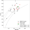 |
Fig. 1 G0 versus (GBP − GRP)0 diagram of the sample. The stars exhibiting Hα emission are reported in red. The green star symbol is the Li-rich star. The CMD is superimposed to the 12 Gyr BASTI isochrones (Pietrinferni et al. 2021) with metallicities [Fe/H] = −1.0 (solid grey line) and [Fe/H] = −2.0 (dashed grey line). |
3.2 Kinematics
We evaluated the kinematics of the target stars using the astrometric data (coordinates, proper motions, parallaxes) and radial velocities (RVs) from Gaia DR3 (Gaia Collaboration 2023), together with the galpy code2 (Bovy 2015).
We adopted the default MWPotential2014 Milky Way potential (Bovy 2015), solar distance, and circular velocity at the solar distance of r0=8 kpc, v0=220 km s−1 (Bovy et al. 2012) and the solar motion from Schönrich et al. (2010). To evaluate the errors on the calculated quantities, similarly to Bonifacio et al. (2021), we employed the pyia code (Price-Whelan 2018). We extracted, for each star, one thousand realizations of the six input parameters, using multivariate Gaussians, as well as the errors in the input parameters, and taking into account the covariance matrix between the astrometric parameters.
Parallaxes were zero-point corrected following the prescription of Lindegren et al. (2021)3. The Gaia DR3 catalog does not report RVs for stars TYC 5422-1192-1 and CD-52 2441. For these stars, we adopted the RVs measured from the UVES spectra. A negative parallax is assigned to star CD-35 14807 in Gaia DR3. For this star, we adopted the photogeometric distance from Bailer-Jones et al. (2021).
Following Bensby et al. (2014), our targets can be divided into 42 with thin disk kinematics, 22 belonging to the thick disk, and one of transition type between them. Then, 34 stars are classified as belonging to the halo. Among the halo stars, six and three are kinematically similar to the Gaia-Sousage-Enceladus (GSE, Belokurov et al. 2018; Haywood et al. 2018; Helmi et al. 2018) and the Sequoia (Seq., Barbá et al. 2019; Myeong et al. 2019; Villanova et al. 2019) structures, respectively, according to the criteria introduced by Feuillet et al. (2021). We report in Tables B.3 and B.4 (available at the CDS) some of the property evaluated for the target stars and their classification (where class: (1) thin disk; (2) thick disk; (3) thin-thick transition; (4) halo; (5) GSE candidate; and (6) Seq. candidate).
Putting the focus on the 32 metal-poor stars, none of these belong to the thin disk or they are in transition between the thin and thick disk. The whole sample can be divided into halo (23) and thick-disk (9) stars. Moreover, among the halo stars, four and two are kinematically similar to GSE and Seq., respectively.
The top panels of Fig. 2 present the target stars in the Galactocentric cartesian Z versus cylindrical radius R plane (top-left), in the Galactocentric Cartesian Y versus X plane (top-middle) and in the maximum height over the Galactic plane Zmax versus the apocentric distance, rap, plane (top-right). The bottom-left panel presents stars in the pericentric distance rperi versus rap plane. The bottom-middle and bottom-right panels are a zoom-in of the top-right and bottom-left panels, respectively. The identity lines are also plotted in these panels to indicate the forbidden region above the line in the bottom-middle panel, and the locus of stars with zero eccentricity (rperi=rap) in the bottom-right panel.
Stars classified as belonging to the thin disk (magenta), thick disk (cyan), thin-thick transition (blue), and the halo (black) are marked as filled circles. Candidate GSE and Seq. members are marked with red squares and green diamonds, respectively.
Target stars are confined to distances lower than 3.7 kpc from the Sun, they reach out to about 10 kpc in the disk from the Galactic center and are found within 2.5 kpc from the plane (top panels). The middle panels reveal that a few stars classified as halo and GSE reach large Zmax and rap. Halo and GSE stars get to smaller rperi distances than Seq., thick-disk, transition, and thin-disk stars. This is due to the progressively lower eccentricity of the orbits of these objects, which can be better appreciated looking at the distance from the identity line (zero eccentricity: rperi=rap) of the different categories of objects in the bottom-right panel. We notice that Seq. candidates have extremely retrograde orbits which are, however, less eccentric than halo and GSE stars (see bottom-left panel in Figure 3).
While three halo and two GSE stars reach Zmax > 10 kpc, the rest of the halo stars are confined to Zmax < 7 kpc (bottom-left panel); therefore, they belong to the inner halo population. Most of the thin disk stars have Zmax < 1 kpc, but a few stars extend to Zmax ≃ 2 kpc. Star classified as thick disk extend to Zmax up to 4 kpc and Seq. stars to Zmax < 3 kpc. We notice that the classification between thin-disk, thick-disk, transition, and halo stars is based on their current Ulsr,Vlsr, and Wlsr velocity components.
Figure 3, presents the target stars in several commonly used planes to characterize the stellar orbits and kinematics (Lane et al. 2022), using the same symbols as in Fig. 2. The background gray dot population is the “good parallax sub-sample” studied in Bonifacio et al. (2021), which we use here for reference only.
The top-left and top-middle panels present a version of the Toomre diagram (square root of the sum of the squares of the radial VR and vertical VZ velocity components in galactocen- tric cylindrical coordinates vs the transverse velocity component, VT) and the VT versus VR plane, first used to identify the “Sausage” structure by Belokurov et al. (2018). The top-right panel is the usual total orbital energy E versus angular momentum LZ plane. The bottom-panels present the eccentricity versus LZ (left), the square root of the radial action JR vs the azimuthal action (Jϕ=LZ, middle) and the so called action diamond (right), namely the difference between the vertical and radial actions (JZ − JR) vs Jϕ, both normalized to the total action Jtot=JR+|Jϕ|+JZ. In the bottom-middle and bottom-right panels, the red and green shaded areas indicate the criteria adopted here from Feuillet et al. (2021) to select candidate GSE and Seq. stars; namely, −500<LZ < +500 kpc km s−1 and  (kpc km s−1)1/2 for GSE and (JZ − JR)/Jtot < 0.1 and Jϕ/Jtot < −0.6, for Seq., respectively.
The different classes of objects are perhaps better separated in these planes. Thin-disk, transition, and thick-disk stars have prograde orbits (VT or LZ > 0). Moving from thin- to thick-disk stars, the eccentricity of the orbits increases, together with JR, VR, and VZ, while LZ =Jϕ, E and VT all decrease. Seq. stars have the most retrograde orbits in the sample.
Halos stars have, as expected, together with GSE stars, the most eccentric orbits. Including the GSE and Seq. candidates, 21 out of 34 halos stars have prograde orbits. These number change to 18 out of 25 on prograde orbits, excluding the 9 stars belonging to GSE (6) and Seq. (3). GSE stars have prograde and retrograde orbits in equal number (3). Considering only stars having Zmax < 7 kpc (and therefore rap < 50 kpc,  kpc km s−1, and E< 04, see Figs. 2 and 3), then we are left with 17 out of 22 (77%) stars on prograde orbits. This is consistent with these stars participating in a collapse process which gave rise to the inner halo and with the mostly prograde orbits (70%) found in very metal-poor stars ([Fe/H] < −2) at 1 < |Z | < 3 kpc by Carter et al. (2021) using data of the H3 survey.
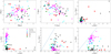 |
Fig. 2 Top-left: galactocentric Cartesian height over the galactic plane Z vs. cylindrical galactocentric radius R. Top-middle: targets’ Galactocentric Cartesian Y vs. X coordinates. Top-right: maximum height over the galactic plane Zmax vs. apocentric distance rap. Bottom-left: pericentric distance rperi vs. rap. Bottom-middle: zoom-in of the top-right panel. The region above the line is forbidden. Bottom-right: zoom-in of the bottom-left panel. The stars with zero eccentricity lie on the line rperi =rap. Targets classified as belonging to the thin- (magenta) or thick-disk (cyan), thin-thick transition (blue), and halo (black) are presented as filled circles. Candidate GSE and Seq. stars are denoted with red squares and green diamonds, respectively. |
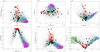 |
Fig. 3 Top-left: Toomre diagram ( Top-middle: VT vs. VR. Top-right: orbital energy E vs. angular momentum LZ. Bottom-left: orbital eccentricity vs. LZ. Bottom-middle: |


3.3 Abundances
We estimated the chemical abundances of the elements up to zinc using MyGIsFOS. Regarding n-capture elements measurements, we used the Wrapper for Turbospectrum and Fitprofile (WTF), a Python code that computes line profile fits from a synthetic spectra grid computed on the fly. From an input file defining the region(s) for line fitting and continuum pseudonormalization, the input atmosphere model, the observed spectrum to fit and the ion and abundance range for the calculation, WTF calls on turbospectrum (Alvarez & Plez 1998; Plez 2012) to compute a grid of small synthetic spectra around the region of interest, then launches Fitprofile (Thygesen et al. 2016) to compute the best-fitting synthetic. In this case, Fitprofile was run with the abundance of the element of choice as the only free parameter. Finally, WTF displays the fit result graphically.
In the present case, ATLAS9 (Kurucz 2005) models were computed for the parameters and the MyGIsFOS-derived abundance pattern for every star (elements for which we derived abundances in MyGIsFOS were put at the derived values, the others were set to the solar-scaled value for the star’s metallic- ity). WTF retains the Fitprofile capability to fit different features for the same ion either as separate, or as a single global fit. In this work, if multiple lines were present, each one was fitted separately.
In Table B.5 (available at the CDS), we provide the line list adopted (value 1) for each star. The average abundances obtained are listed in Table B.6 (available at the CDS). The error reported is the line-to-line scatter (σ). However, to get the final error, the uncertainties due to atmospheric parameters should be added in quadrature. We estimated these last uncertainties for the star BD-11 3235 by varying ∆Teff = ±100 K, ∆ log ɡ = ±0.2 dex, and ∆ξ = ±0.2 km s−1. We considered this star because its atmospheric parameters are representative of the sample and all the elements have been measured for it. The typical errors due to atmospheric parameters are reported in Table 1 for all chemical species analyzed here. Similar results have been found for the first sample of metal-poor giant stars analyzed by the MINCE collaboration (Cescutti et al. 2022; François et al. 2024, hereafter the MINCE I sample). The solar abundances adopted in this work are listed in Table 2. Finally, we want to highlight that we used [X/Fe] = [X/Fe I] or [X/Fe] = [X/Fe II] when X is a neutral or ionised species, respectively.
The sulfur abundances A(S) were measured following a different procedure. In the wavelength ranges covered by the spectral frames centered at 580 and 760 nm lie the Sulfur (S) lines of Mult. 6, 8, and 1. These lines are of high excitation, thus, they become weak at low temperatures and in the metal-poor regime. We rejected the S lines at bluer wavelengths (Mult. 6, 8) because too weak, and we considered only the strongest features at 920 nm (Mult. 1). The contamination due to telluric lines in this wavelength region makes difficult the standard workflow of MyGIsFOS. In particular, the pseudonormalization of the observed spectrum is hampered when a telluric line falls in a continuum region. Moreover, since MyGIsFOS does not take into account the presence of telluric lines, blended or shape distorted lines are not recognized by the code. Therefore, depending on the degree of telluric contamination, MyGIsFOS rejects S lines or overestimates the abundances. For these reasons, we decided to derive A(S) from equivalent width (EW).
We first compared the observed spectra of our stars with that of a B-type star to evaluate the suitability of Mult. 1 lines. S lines contaminated by telluric lines were rejected. This reduced our sample to a total of 23 stars. Using the deblending option of the IRAF5 task splot, we took into account the contribution in EW from the telluric and S lines. The conversion from EW to abundances was computed through the GALA code (Mucciarelli et al. 2013), which is a user-friendly wrapper for WIDTH9 (Kurucz 2005). The results obtained for sulfur are reported in Table B.7 (available at the CDS).
Sensitivity of abundances on atmospheric parameters.
Solar abundances used throughout this paper.
3.4 Non-local thermodynamic equilibrium effects
Among the elements analyzed in this work, some are known for being sensitive to deviation from LTE, or NLTE effects. In this work, the chemical investigation was performed under the assumption of LTE, similar to what done in the first two papers of the series: Cescutti et al. (2022) and François et al. (2024). The intervals in metallicity, effective temperature, and surface gravity spanned by the present sample is similar to that of the sample analysed in Cescutti et al. (2022) and François et al. (2024). We defer to more complete analysis of the NLTE effects to a future investigation on the complete sample. To provide an indication of the magnitude of NLTE effects we are dealing with, as reported in Cescutti et al. (2022), we took advantage of the thorough investigation by Hansen et al. (2020). In Table 9 of Cescutti et al. (2022), we provide the NLTE corrections from Hansen et al. (2020) for BD-10 3742 (Teff, log ɡ, [Fe/H], ξ: 4678 K, 1.38, −1.96, 1.9 km s−1) and BD-12 106 (4889 K, 2.03, −2.11, 1.5 km s−1). These two stars have parameters that are close to those of BD +07 4625 and BD +39 3309 in the MINCE I sample and to those of CD-52 976 (4655 K, 1.29, −1.90, 1.97 km s−1) and BD-19 3663 (4767 K, 1.82, −2.51, 1.82 km s−1) in the present sample. We therefore refer the reader to the discussion in Cescutti et al. (2022) and Table 9 to have an indication of the NLTE corrections we should be dealing with. Another relevant paper is Matas Pinto et al. (2021), who provided NLTE corrections for two stars with stellar parameters similar to the stars investigated here. From this comparison, we conclude that for all elements, except Na I and Co I, the NLTE corrections are smaller than the typical uncertainty on the abundances and they are positive; NLTE corrections for Fe become even smaller when using [X/Fe]. Therefore, the comparison of LTE abundances with chemical evolution models is meaningful. There are not many NLTE computations available for neutron capture elements, but a discussion of NLTE corrections for Sr, Eu, and Ba can be found in François et al. (2024).
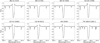 |
Fig. 4 Spectra of the Hα line of the stars exhibiting P-Cygni and/or inverse P-Cygni profile. |
4 Discussion
In the following section, we present the results obtained for the MINCE III stars.
4.1 Stars exhibiting Hα emission
We realised that some stars in the sample show P-Cygni and/or inverse P-Cygni profile, a signature of stellar activity. In Figure 1, the stars with activity (red dots) are among the brightest and reddest in the sample, as expected by Smith & Dupree (1988, as reported their Figure 1).
The stars in question are: BD-11 3235, BD-13 934, BD-15 5449, CD-28 17446, CD-33 15063, CD-39 9313, HD 19367, and TYC 8633-2281-1. The spectra of the Hα line of these stars are shown in Figure 4. BD-11 3235 is the only star with symmetric Hα emission wings. In BD-13 934, CD-28 17446, CD-33 15063, and HD 19367, the blue wing is stronger than the red one, while the remaining stars display the opposite profile.
Finally, for these active stars, one must be cautious not to use lines whose contribution also comes from the chromosphere, such as the Ca II triplet lines, the Na I-D lines or the K I line at 769.9 nm, lines that have not been used in this investigation.
4.2 Li-rich star: CD-28 10039
The star CD-28 10039 has A(Li) = 1.1, which is not expected for a star of this log ɡ. According to our kinematic results, this star belongs to the thick disk.
To check the evolutionary state of this star, we considered two BASTI isochrones (Pietrinferni et al. 2021) characterized by [Fe/H] = −1.0 and −2.0, [α/Fe] = +0.4, and age = 12 Gyr. In Figure 1, CD-28 10038 (green star symbol) lies close to the asymptotic-giants branch of the isochrone with [Fe/H]=−1.0.
We reported CD-28 10039 in the A(Li) versus log ɡ diagram (green star symbol in Figure 5). The evolution of Li with log ɡ is characterized by the Spite plateau (A(Li) ∼ 2.2 dex, Spite & Spite 1982), followed by the first dredge-up (FDU) drop until the RGB Plateau (A(Li) ∼ 1 dex, Mucciarelli et al. 2012, 2022), which is followed by another drop due to the RGB bump (RGBb) mixing episode. In this diagram, the unexpected position of CD- 28 10039 (slightly above the RGB Plateau at low log ɡ) reveals that the Li enhancement of this star is not due to standard stellar evolution (Iben 1967) or non-canonical mixing processes (Charbonnel et al. 2020; Magrini et al. 2021).
The spectra of CD-28 10039 (red) are compared with those of the star with similar parameters CD-27 16505 (black) in Fig. 6. The top panel shows the evident difference in strength of the Li line at 670.78 nm between the two stars. The reddest line of the Mg II triplet at 518.36 nm seems similar in both stars (second panel from the top), suggesting that the Li enhancement of CD-28 10032 is not due to rotation effects. The Hα and the reddest line of the Ca II triplet at 866.21 nm are reported in the last two panels. From these two features it is possible to notice slight differences between the Li-rich and the reference stars. The Hα of the Li-rich star seems shallower, with asymmetrical core and blue wing. On the other hand, the red wing of the reddest line of the Ca II triplet appears shallower in the Li-rich stars than in the reference one. These anomalous profiles could be compatible with chromospheric activity and mass loss (Meszaros et al. 2008). However, the Hα blue wing of CD-27 16505 suggests a slight emission profile, so it could be possible that we are comparing two active stars in this case.
From the chemical point of view, CD-28 10039 has A(Y) = 1.17 ±0.00 and A(Ba) = 1.34 ± 0.09. These values are not discrepant with those of the sample. For instance, we obtained A(Y) = 1.01 ± 0.10 and A(Ba) = 1.14 ± 0.00 in CD-27 16505. Comparing the abundances of the s-process elements, for the Li-rich star, the ratio [Rb/Y] = −0.06 dex suggests a low neutron density at the sites of these elements (Smith & Lambert 1984). Moreover, we find a similar r-process elements enrichment for the Li-rich star of A(Eu)=0.04 dex, and CD-27 16505 of A(Eu)=0.05 dex.
We present in Figure 7 the spectral energy distribution (SED, red and yellow points) of CD-28 10039, which we constructed using the Virtual Observatory SED Analyzer (VOSA6, Bayo et al. 2008) service. The SED was generated adopting the stellar distance and extinction, namely d=2.14 kpc and AV = 0.22 mag. We fit the SED using Kurucz ATLAS9 model atmospheres calculated with new opacity distribution functions and no overshooting (Castelli & Kurucz 2003), allowing for a narrow range of parameters, that is, around those we adopted here for the star. The best-fitting model (blue points and line), obtained with the parameters indicated in the top-label of the figure, appears to be a fair representation of the stellar SED all over the wavelength range, but for the NUV Galaxy Evolution Explorer (GALEX) photometry at 2303.37 Å. In fact, CD-28 10039 appears to present a significant NUV excess, which may be indicative of the presence of a hot companion, such as a white dwarf.
On the other hand, the radial velocity measured from the UVES spectra and that reported in Gaia DR3, are very similar to each other (RV difference of less than 0.5 km s−1 ). Furthermore, the Gaia DR3 astrometry quality parameters are not suggestive of binarity: RUWE=1.13, astromet- ric_gof_al=2.79, astrometric_excess_noise = 0.09 mas, although astrometric_excess_noise_sig = 10.1. Finally, Gaia DR3 has not reported any variability information for CD-28 10039 (phot_variable_flag=“NOT_AVAILABLE”). However, the star has been reported as variable in G, GBP, and GRP (VarF=VVV), according to the analysis of Maíz Apellániz et al. (2023).
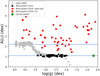 |
Fig. 5 A(Li) versus log g diagram for CD-28 10039 in comparison with literature data: Lind et al. (2009, grey), Mucciarelli et al. (2022, black), Mucciarelli et al. (2024, red). The blue lines are the Spite (A(Li) ∼ 2.2, Spite & Spite 1982) and RGB (A(Li) ∼ 1.1, Mucciarelli et al. 2012) plateaus. |
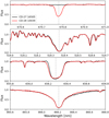 |
Fig. 6 Comparison of the spectra of the Li-rich star CD-28 10039 (red) with that of CD-27 1605 (black) in different wavelength regions. From the top to bottom: Li doublet at 670.78 nm, reddest line of the Mg II triplet at 518.36 nm, Hα at 656.28 nm, and the reddest line of the Ca II triplet at 866.21 nm. |
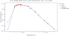 |
Fig. 7 Spectral energy distribution of CD-28 10039 obtained from the VOSA service. The model obtained with the parameters indicated in the toplabel is shown in blue. An apparent NUV excess has been detected from GALAX photometry. |
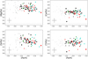 |
Fig. 8 α-elements abundances measured in the MINCE III stars. Black and cyan points are Galactic stars belonging to the halo and thick-disk, respectively. Candidate Gaia–Sausage–Enceladus (red squares) and Seq. (green diamonds) stars are also shown. The results of Cescutti et al. (2022) for the same substructures in the MINCE I sample are reported with same colors and smaller symbols. The gray points are the results of Lombardo et al. (2022). |
4.3 α-elements
Figure 8 shows our results for the α-elements Mg, Si, Ca, and Ti. The stars belonging to the Galactic halo (black dots), Galactic thick-disk (cyan dots), GSE (red squares), and Seq. (green diamonds) substructures are distinguished by colors and symbols. The good agreement with the first results of the MINCE series (Cescutti et al. 2022) is shown adopting the same colors and smaller symbols. As comparison, we report the results of Lombardo et al. (2022) obtained from the CERES survey in gray. This legend will be maintained for the rest of the section.The stars of the different substructures seem to share the same plateau trend in all panels in the metallicity range −2.5 < [Fe/H] < −1.5. Moreover, due to the low number of GSE, and Seq. stars, it is not possible to draw further conclusions about the differences between MW, GSE, and Seq. members.
All the α-elements are enhanced with respect to the [Fe/H] abundances with sample averages and standard deviations of ⟨[Mg/Fe]⟩ = 0.49 ± 0.08, ⟨[Si/Fe]⟩ = 0.39 ± 0.09, ⟨[Ca/Fe]⟩ = 0.36 ± 0.09, and ⟨[Ti/Fe]⟩ = 0.34 ± 0.09. We also estimated the [Ti II/Fe II] ratio. In particular, the mean abundances ratio is 0.42 ± 0.14, and the mean difference between [Ti II/Fe II] and [Ti I/Fe I] is 0.08 ± 0.14. The NLTE effects for Ti I lines (Mashonkina et al. 2016) may explain the fact that the ionization equilibrium of Ti has not been established, although the offset is not very significant. These results are in agreement, within the errors, with those in the literature (see e.g. Cescutti et al. 2022; Lombardo et al. 2022).
Figure 9 compares the sulfur results before (left panel) and after (right panel) NLTE corrections. In the left panel, we can guess the presence of a plateau at the value [S/Fe]LTE ∼ 0.64. This quantity is considerably higher than both the usual [α/Fe] ∼ 0.40 and [S/Fe] ∼ 0.30 values in the literature (Caffau et al. 2010; Nissen et al. 2007). After NLTE corrections, the [S/Fe] ratios present a larger scatter but the plateau value, ⟨[S/Fe]⟩ = 0.45 ± 0.19, is in better agreement with the typical [α/Fe] abundance ratio. The large scatter in [S/Fe] is introduced by the difficulties in the A(S) estimation, such as the telluric contamination and the NLTE corrections.
In Figures 8 and 9, we notice a peculiar star with low α-elements content. The MW halo star CD-38 13823 is Mg-rich ([Mg/Fe]=0.49), as expected for its metallicity ([Fe/H] = −2.46), whereas it is slightly poor in [Si/Fe]=0.27 and [S/Fe]=0.26, and with solar ratios of [Ca/Fe]=0.06 and [Ti/Fe]=0.06.
4.4 Light-odd elements
Figure 10 shows our results for the light-odd elements Na, Al, Sc, and V. The stars of the different kinematic components are identified with the same colors and symbols as in Fig. 8. In the following, we comment on which lines were used to determine the abundances in the MINCE III sample.
The Na abundances were derived from the Na I lines at 498.3 nm, 568.2 nm 568.8 nm, the Na D resonance lines at 588.9 nm (D1) and 589.5 nm (D2), and 616.1 nm. The large dispersion < [Na/Fe] >= −0.08 ± 0.15 may be due to the LTE deviations of these lines. In our sample, three halo stars, two thickdisk stars, and one Seq. candidate are Na-rich. However, the limited size of the sample does not allow us to draw any robust conclusion about the differences between MW and GSE stars.
The A1 abundances were derived from the Al I resonance lines at 394.4 nm and 396.1 nm as well as from the Al I lines at 555.6 nm, and the doublet at 669.6 nm and 669.8 nm. However, the Al I resonance lines were rejected for most of the stars to estimate the final Al abundances. Inspection of Fig. 10 shows that the [Al/Fe] ratio is quite scattered spanning a range of almost 0.8 dex. The mean value is ⟨[Al/Fe]⟩ = 0.16 dex, with a standard deviation of 0.26 dex. The dispersion is driven by four Al-enhanced stars, two of which belong to the MW halo, one to the MW thick-disk, and one to GSE. The MINCE I sample shows similar scatter and dispersion. In Fig. 10, the [Na/Fe] and [Al/Fe] ratios do not show clear trends with the metallicity.
We determined the mean abundance ratios of Sc and V ions to the corresponding Fe ions. The ratios and their corresponding standard deviations are: ⟨[Sc I/Fe I]⟩ = −0.01 ± 0.13, ⟨[Sc II/Fe II]⟩ = 0.28 ± 0.15, ⟨[V I/Fe I]⟩ = −0.01 ± 0.08, and ⟨[V II/Fe II]⟩ = 0.02 ± 0.15. Thus, while the mean difference between [Sc IIFe II] and [Sc I/Fe I ]is about 0.29 ± 0.17, the one between [V II/Fe II] and [V I/Fe I] is only of 0.03 ± 0.17. These results agree within errors with those obtained by Lombardo et al. (2022) in a sample of lower metallicity giant stars. We noticed a slight increase in the [Sc II/Fe] and [V I/Fe] ratios with metallicity.
In Fig. 10, CD-38 13823 displays a low [Sc/Fe] ratio of about −0.17 and it is slightly poor in [Na/Fe] = −0.38 and [V/Fe] = −0.26. We were not able to measure the Al abundance for this star.
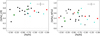 |
Fig. 9 [S/Fe] versus [Fe/H] LTE (left panel) and NLTE (right panel) diagrams of the MINCE sample, the MINCE I (Cescutti et al. 2022) sample is identified by smaller symbols. Colors and symbols are the same as in Figure 8. |
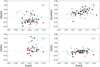 |
Fig. 10 Light-odd elements abundances measured in the MINCE stars, the MINCE I sample (Cescutti et al. 2022) is identified by smaller symbols. Colors and symbols are the same as in Figure 8. |
4.5 Iron-peak elements
Figure 11 shows our results for the iron-peak elements Cr, Mn, Co, Ni, Cu, and Zn. The first five of these elements are produced in nuclear statistical equilibrium in SNe of all types, such as iron, so their ratios to iron are expected to be close to the solar value. The situation is less clear for Zn, that may have contribution from α-rich freeze-out and from neutron captures (see Duffau et al. 2017, for a discussion on the nucleosynthesis of Zn). In the MINCE III sample Cr, Ni, Co, and Zn have mean abundance ratios close to solar: <[Cr/Fe]) = 0.00 + 0.06, <[Co/Fe]> = 0.09 + 0.06, <[Ni/Fe]> = 0.00 + 0.03, and <[Zn/Fe]> = −0.02 + 0.13. Here, Co and Ni display flat trends, while Cr and Zn exhibit increasing and decreasing trends with metallicity, respectively. Previous studies have found similar behavior for these elements (Cayrel et al. 2004; Bonifacio et al. 2009; Ishigaki et al. 2013; Cescutti et al. 2022; Lombardo et al. 2022).
The iron-peak elements showing exceptional behavior are Mn and Cu. Indeed, we observed sub-solar trends for these elements, which slightly increase with metallicity. Similar behaviors have been noted by Ishigaki et al. (2013) and Cescutti et al. (2022).
Manganese is produced by both SNe Ia and SNe II, like the other iron peak elements; however, the contribution by SNe la at solar metallicity is higher compared to iron, leading to a speculate trend to that of the α-elements. Moreover, Mn yields from SNe la are the most dependent to the explosion mechanism among the iron peak elements and its evolution can be used to evaluate the presence and contribution of different SNe la channels (Cescutti & Kobayashi 2017; Seitenzahl et al. 2013). The nucleosynthesis of Cu is also peculiar. According to Timmes et al. (1995), the explosion of massive stars at solar metallicity produces yields that are five times higher than the same explosion at low metallicity. Therefore, it is the metal dependencies of SNe II that produce the rise rather than the SNe type-Ia. The behavior of Mn may also be due to the strong NLTE effects on the lines of these elements (Bergemann & Gehren 2008). However, the use of NLTE corrections decreases the trend with metallicity, but does not cancel it, suggesting that SNe la play a role in Mn nucleosynthesis (Eitner et al. 2020). Among the stars of the MINCE III sample, CD-38 13823 is the most Mn-rich, [Mn/Fe] = −0.10, and the most Cu-poor, [Cu/Fe] = −0.78. This star does not show peculiar values for the other iron-peak elements in comparison to the other targets.
The mean abundance ratios and their standard deviations for Mn and Cu ions to the corresponding Fe ions are: <[Cr I/Fe I]> = 0.00 + 0.06, <[Cr II/Fe II]> = 0.11 + 0.12, <[Mn I/Fe I]> = −0.27 + 0.07, <[Mn II/Fe II]> = −0.23 + 0.06. Thus, the ionisation equilibrium is reached in LTE for both Cr and Mn. Our results are in perfect agreement with those found by Lombardo et al. (2022).
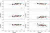 |
Fig. 11 Iron-peak elements abundances measured in the MINCE stars, the MINCE I sample (Cescutti et al. 2022) is identified by smaller symbols. Colors and symbols are the same as in Figure 8. |
4.6 Neutron capture elements
Figure 12 displays our results for the n-capture elements Rb, Sr, Y, Zr, Ba, La, Ce, Pr, Nd, Sm, and Eu. The different MW substructures are shown with the same colors and symbols as in Figure 8. The gray points are from Lombardo et al. (2022); Lombardo (2023). Our results are generally in agreement with the analysis of the MINCE I sample (smaller symbols François etal. 2024).
We observed flat trends for all the n-capture elements with the exception of Sr and Ba, whereby Sr decreases with increasing metallicity, while Ba increases. Similar behaviors have also been noted in other studies (François et al. 2007; Ishigaki et al. 2013; Lombardo et al. 2022). In particular, we found sub-solar mean abundances ratios and standard deviation for ⟨[Sr/Fe]⟩ = −0.41 ± 0.28. The mean abundances of ⟨[Y/Fe]⟩ = −0.09 ± 0.19, ⟨[La/Fe]⟩ = 0.08 ± 0.22 and ⟨[Ce/Fe]⟩ = 0.01 ± 0.21 are close to solar. Finally, we found mean abundances above solar for ⟨[Zr/Fe]⟩ = 0.38 ± 0.21, ⟨[Ba/Fe]⟩ = 0.13 ± 0.26, ⟨[Pr/Fe]⟩ = 0.11 ± 0.17, ⟨[Nd/Fe]⟩ = 0.16 ± 0.21, ⟨[Sm/Fe]⟩ = 0.31 ± 0.19, and ⟨[Eu/Fe]⟩ = 0.43 ± 0.21.
Considering both the MINCE I (François et al. 2024) and the present samples, we find an indication of a slight increase in the n-capture elements scatter with decreasing metallicity. This is more visible in the trends of Ba, La and Eu. The comparison with the results of Lombardo et al. (2022); Lombardo (2023) allows to better visualize this effect. The MW, GSE and Seq. stars seem to behave similarly for all elements (see Fig. 12). However, a larger sample for each substructure is required to draw firmer conclusions.
The s-process elements content of CD-38 13823 is low: [Y/Fe] = −0.70, [Zr/Fe] = −0.39, [Ba/Fe] = −0.72, [La/Fe] = −0.49. On the other hand, in comparison to the other stars of the sample, it is also the poorest one in [Sm/Fe] = −0.24 and [Eu/Fe] = −0.03.
The [Eu/Ba] versus [Ba/H] diagram in Fig. 13 allowed us to discriminate the origin of the n-capture elements enrichment.
In this plot, the (almost) Eu-free stars lie at [Ba/H] ≤ −3 (Cescutti et al. 2015; Cavallo et al. 2021), the enrichment in the range −2.5 < [Ba/H] < −1.5 may be attributed to rotating massive stars, while AGB stars are likely responsible for the enrichment at [Ba/H] > −1. The r-process pollution occurs at [Eu/Ba] > 1. Our sample of stars appears to define a flat trend up to [Ba/H] ∼ −1.0. The Li-rich star, CD-28 10039, lies in the area polluted by AGB stars, while the position of the peculiar star, CD-38 13823, supports its low Eu-content.
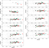 |
Fig. 12 Neutron capture elements abundances measured in the MINCE stars, the MINCE I sample (François et al. 2024) is identified by smaller symbols. Colors and symbols are the same as in Figure 8. The stars of the CERES survey analyzed by Lombardo et al. (2021); Lombardo (2023) are reported in gray. |
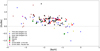 |
Fig. 13 Abundance ratio of [Eu/Ba] as a function of [Ba/H] for MINCE stars. MW halo, Seq., and GSE stars are reported as black dots, green diamond symbols, and red square symbols, respectively. The results for MINCE I stars (François et al. 2024) are represented with same color and smaller symbols. The Li-rich star CD-28 10039 (green) and CD- 38 13823 (magenta) are highlighted with star symbols. We added the samples from Ishigaki et al. (2013) for comparison. |
5 Chemical evolution model
We compare our results with a stochastic chemical evolution model (Cescutti & Chiappini 2014; Cescutti et al. 2015) that traces Rb, Sr, Y, Zr, Ba, La, and Eu as well as the α elements Mg, Ca, Si, Ti, the light-odd element Sc, and the iron peak elements Mn, Co, Ni, and Zn.
The chemical evolution model presented in Figures A.1 and A.2 is the same as described in Cescutti & Chiappini (2014). The model describes the evolution of the Galactic halo and assumes a stochastic formation of stars, it consists of 100 realizations, each of them with the same parameters of chemical evolution (infall, outflow, star formation efficiency, initial mass function, etc). In each region, the following gas infall law with a primordial chemical composition was applied:
 (1)
(1)
where to is set to 100 Myr and σo is 50 Myr. Similarly, the star formation rate is defined as
 (2)
(2)
where ρɡas (t) represents the gas mass density within the volume under consideration. Additionally, the model includes an outflow from the system:
 (3)
(3)
In each volume, at each time step, the masses of the stars are assigned with a random function, weighted according to the same initial mass function. In this way in each region, at each time step, the mass of gas turned into stars is the same, but the total number and mass distribution of the stars are different. This produces different chemical abundances, which are even stronger if there are large differences among the yields of the stellar masses (Cescutti 2008). The other stochastic events include enrichment by magneto-rotational driven supernovae (Nishimura et al. 2015), which are the events producing n- capture elements through the r-process in our model. Similar results can be obtained also assuming neutron star mergers with very short time delay (see Cescutti et al. 2015). Therefore, some volumes may be enriched early on by an r-process event, while others are only enriched later, producing a dispersion in the traced n-capture elements. In this model, besides the enrichment due to r-process events, the n-capture elements are considered produced by rotating massive stars, assuming the yields by Frischknecht et al. (2016). The use of different yields does not alter the outcome substantially (Rizzuti et al. 2021). The other source of neutron capture elements, asymptotic giant branch stars, is also included by adopting yields from Cristallo et al. (2011). All the details can be found in Cescutti & Chiappini (2014). The nucleosynthesis for the remaining elements, namely α- and iron-peak elements, is based on François et al. (2004). They slightly altered the original yields presented in Woosley & Weaver (1995) to match, with a standard chemical evolution model, the abundances in extremely metal-poor stars measured in Cayrel et al. (2004). The only variation for these yields concerned nickel. The original results produced a [Ni/Fe] ∼ 0.3 at [Fe/H] = −2, visible in François et al. (2004) as well as Cescutti et al. (2022). According to the present results, nickel should be decreased by a factor of two in a new implementation of this model.
The comparison of our chemical evolution model for elements Mg to Zn of the MINCE sample (that includes also the star in the MINCE I sample), shown in Figs. A.1 and A.2, is by and large, satisfactory. Some concern is on Zn, for which the observed dispersion in abundance ratios is larger than what predicted by the model. Another cause of concern is for Co I, if a NLTE correction of the order of +0.5 dex, as suggested by Hansen et al. (2020) is applied, the [Co/Fe] ratios are all well above the model predictions. We do not provide a comparison of the model with the data for Na I, because this element is not currently included in our model. We refrained from performing any quantitative comparison of the model with the observations and defer such an exercise to the time when a larger sample of analysed stars becomes available.
The primary goal of MINCE is to provide abundance ratios for neutron-capture elements in intermediate metal-poor stars (−2.5 < [Fe/H] < −1.5), offering crucial constraints on model development to distinguish between different nucleosynthesis scenarios. In Figure A.2, we compare model predictions with the MINCE III data for neutron-capture elements (X = Rb, Sr, Y, Zn, Ba, La, and Eu) presented in this study. Notably, the spread in model predictions in the [X/Fe] versus [Fe/H] space shrinks at higher metallicities and within the metallicity range of the MINCE data, the model’s predicted [X/Fe] dispersion is well aligned with the observations. This agreement supports the validity of the adopted nucleosynthesis prescriptions and the model assumptions. At the same time, iron peak elements and α-elements dispersion are very reduced in the abundance measurements and compatible at this metallicity with the one proposed by the model results. Moreover, this is the first time that we can confirm the model predictions for rubidium shown in Cescutti et al. (2015), at that time there were not stellar abundances measurements for this element in halo stars. We also note that europium predictions are slightly too high compared to the measured data. This is most likely connected to the simplified assumptions for the r-process yields, which scale among the elements as the observed pattern in r-process-rich stars. This offset was visible also in the original results (Cescutti & Chiappini 2014). Barium shows some stars located above the model results, but for lanthanum, which has a very similar nucleosynthesis, the comparison between abundance measurements and model results is excellent. Small offsets are visible for Zr and Y as well.
6 Summary and conclusions
The MINCE project investigates the nucleosynthetic processes that lead to the chemical elements production in the intermediate metallicity range, −2.5 < [Fe/H] < −1.5, with a particular focus on the bulk of elements heavier than iron (Z > 30). In this work, we present an analysis performed with high resolution and high signal-to-noise UVES data of 94 stars. Of these, we provide a detailed chemical inventory for 32 stars, while for the remaining stars, we only provide [Fe/H] and atmospheric parameters; for 5 stars, no abundances or atmospheric parameters are provided. Remarks on individual stars can be found in Appendix C.
All 99 stars observed were kinematically characterized and divided into thin-disk (42), thick-disk (22), thin-to-thick disk (1), and halo (34) stars, where 6 and 3 halo stars belong to GSE and Seq., respectively. Among the subsample of 32 stars with detailed chemical analysis, 23 stars belong to the Galactic halo, 9 to the thick-disk, 4 to GES, and 2 to Seq.
We derived high-precision abundances for light elements (from Na to Zn) and n-capture elements (Rb, Sr, Y, Zr, Ba, La, Ce, Pr, Nd, Sm, and Eu) for the 32 metal-poor stars. These results, along with those reported in the first two papers of the MINCE series (I–Cescutti et al. 2022, II-François et al. 2024), already represent a significant increase of n-capture elements measurements in the intermediate-metallicity range. However, the low number of GSE and Seq. candidates does not allow us to draw firm conclusions on the differences between these sub-structures and the MW halo.
Among the brightest and reddest stars, eight of them exhibit (inverse) P-Cygni profile. We also identified one low-gravity Li- rich star, CD 28-10039, with A(Li) = 1.1. This last belongs to the thick disk and its Li enhancements is not due to the standard stellar evolution or non-canonical mixing processes. According to the SED of this star, the NUV excess may suggest the presence of a hot companion.
Finally, we compared our results with stochastic chemical evolution model of the MW halo. The events considered by the model for the production and the enrichment of n-capture elements are the stochastic formation of stars in the Galactic halo, magneto-rotational driven supernovae yields, and rotating massive stars and asymptotic giant branch stars yields. The good agreement between the chemical abundances and the chemical evolution model proves that the nucleosynthesis processes adopted to describe the origin of the n-capture elements are reliable.
Data availability
The following online Tables are available in electronic form at the CDS via anonymous ftp to cdsarc.cds.unistra.fr (130.79.128.5) or via https://cdsarc.cds.unistra.fr/viz-bin/cat/J/A+A/695/A36:
Table B.1. Coordinates, Gaia magnitudes and radial velocities of the sample.
Table B.2. Reddening, atmospheric parameters and metallicity of the sample.
Table B.3. Targets’ velocity components in galactocentric cylindrical coordinates (VR,VT,VZ), apocentric and pericentric distances (rap, rperi), orbital eccentricities (ecc.) and maximum height over the galactic plane (Zmax).
Table B.4. Total orbital energy (E), angular momentum (LZ), radial and vertical actions (JR, JZ) and classification of the program stars.
Table B.5. Line list adopted.
Table B.6. Abundances and line-to-line dispersion (σ) of elements in their ionisation state in [X/H].
Table B.7. LTE and NLTE sulfur abundances obtained line by line for the MINCE III stars.
Acknowledgements
Support for the author F.L. is provided by CONICYT- 118 PFCHA/Doctorado Nacional año 2020-folio 21200677. We gratefully acknowledge support from the French National Research Agency (ANR) funded project “Pristine” (ANR-18-CE31-0017). PB acknowledges support from the ERC advanced grant No. 835087 – SPIAKID. This work has made use of data from the European Space Agency (ESA) mission Gaia (https://www.cosmos.esa.int/gaia), processed by the Gaia Data Processing and Analysis Consortium (DPAC, https://www.cosmos.esa.int/web/gaia/dpac/consortium). Funding for the DPAC has been provided by national institutions, in particular the institutions participating in the Gaia Multilateral Agreement. This work was also partially supported by the European Union (ChETEC-INFRA, project no. 101008324) This research has used the SIM-BAD database, operated at CDS, Strasbourg, France. This publication makes use of VOSA, developed under the Spanish Virtual Observatory (https://svo.cab.inta-csic.es) project funded by MCIN/AEI/10.13039/501100011033/ through grant PID2020-112949GB-I00. VOSA has been partially updated by using funding from the European Union’s Horizon 2020 Research and Innovation Programme, under Grant Agreement no. 776403 (EXOPLANETS-A). GC acknowledges the grant PRIN project No. 2022X4TM3H ‘Cosmic POT’ from Ministero dell’Università e della Ricerca (MUR). A.M. acknowledges support from the project “LEGO– Reconstructing the building blocks of the Galaxy by chemical tagging” (PI: A. Mucciarelli), granted by the Italian MUR through contract PRIN 2022LLP8TK_001.
Appendix A Additional figures
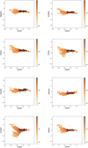 |
Fig. A.1 Comparison between the chemical abundances in MINCE I and III stars and the chemical evolution model for Mg, Ca, Si, Ti, Sc, Mn, Co, and Ni. Colors and symbols are the same as in Figure 8. |
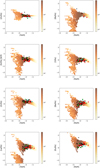 |
Fig. A.2 Comparison between the chemical abundances in MINCE I and III stars and the chemical evolution model for Zn, Rb, Sr, Y, Zr, Ba, La, Eu. Colors and symbols are the same as in Figure 8. |
Appendix B Additional tables
Coordinates, Gaia magnitudes and radial velocities of the sample.
Reddening, atmospheric parameters and metallicity of the sample.
Targets’ velocity components in galactocentric cylindrical coordinates (VR,VT,VZ), apocentric and pericentric distances (rap, rperi), orbital eccentricities (ecc.) and maximum height over the galactic plane (Zmax).
Total orbital energy (E), angular momentum (LZ), radial and vertical actions (JR, JZ) and classification (class, see bottom of the table) of the program stars.
Line list adopted.
Abundances and line-to-line dispersion (σ) of elements in their ionisation state in [X/H].
LTE and NLTE sulfur abundances obtained line by line for the MINCE stars.
Appendix C Remarks on individual stars
C.1 BD–14 52
This star was investigated in the 437+760 wavelength range. It is an active star. According to Gaia DR3 this star is an SB1 binary with a period of 306 days, a radial velocity semi-amplitude of 1.15 km/s and centre of mass velocity of 60.2 km/s close to our adopted radial velocity. The orbit has a low eccentricity of 0.16.
C.2 BD–17 4250
This metal-poor star has been analysed in the 437+760 range, it is active as indicated by Ca II-H and -K emission and P-Cygni (and inverse) profiles on Hα.
C.3 BD–15 4109
This star is metal-poor, it was investigated in the 437+760 range. It is active as implied by the Ca II-H and -K emission and P-Cygni (and inverse) profiles on Hα.
C.4 CD-23 11064
This star is cool, the Mucciarelli et al. (2021) calibration provides and effective temperature of 3748 K we ran it at fixed Teff = 3750 K to avoid extrapolation.
C.5 CD-24 613
This star is cool and was analysed only in the RVS range with the COOL grid. MyGIsFOS required a shift of +5.6 kms−1 with respect to the Gaia radial velocity.
C.6 CD-27 14182
Was analysed in the 437+760 range. There is a tiny emission in Ca II-H and -K lines. No evidence of Li I doublet.
C.7 CD-28 10387
Was analysed in the 437+760 range. Normal Hα, tiny emission in Ca II-H and -K lines. No evidence of Li I doublet.
C.8 CD-29 9391
Was analysed in the RVS range with the COOL grid. Our spectrum required a shift of −1.05 kms−1 with respect to the Gaia radial velocity.
C.9 CD-31 17277
Gaia DR3 classifies it as Long Period Variable (LPV) but does not provide a period.
C.10 CD-32 13158
The star has been analysed in the 437+760 range. Normal Hα, tiny emission in Ca II-H and -K lines. No evidence of Li I doublet. The star is of solar metallicity and has a sizeable rotational velocity. Comparison with the evolutionary tracks of Ekström et al. (2012) implies a mass of 6 M⊙ and an age of 70 Myr.
C.11 CD-34 242
This star is cool and was analysed only in the RVS range with the COOL grid. MyGIsFOS required a shift of +2.6 kms−1 with respect to the Gaia radial velocity.
C.12 CD-35 13334
This star is cool and was analysed only in the RVS range with the COOL grid. MyGIsFOS required a shift of +1.8 kms−1 with respect to the Gaia radial velocity.
C.13 CD-35 13661
According to Gaia this star is an SB1 binary with a period of 2 days and a semi-amplitude of 1.35 kms−1. The centre of mass radial velocity is +59.02 kms−1, very close to our adopted radial velocity. The eccentricity is low, 0.12. Analysed in the 437+760 range. Hα with P-Cygni and emission on Ca II-H and -K lines. No evident feature at the Li I doublet wavelength.
C.14 CD-45 8357
This star is classified as an RS CVn binary in the Gaia DR3 catalogue. Our spectrum does not show a secondary spectrum (as expected for an RS CVn). The radial velocity from our UVES spectrum is −20.5 ± 0.33 km/s, to be compared to the value provided by Gaia −32.39 ± 5.24. Although the two values are compatible at 2.2σ, we consider this as a clear indication that the star’s radial velocity is varying, as is the very large error in the Gaia radial velocity, incompatible with a star of this brightness. The Ca II H& K line show a very strong emission, further supporting the RS CVn classification of this star. A chemical analysis of such a star is beyond the scope of our paper, however from comparison with synthetic spectra we estimate the metallicity to be roughly solar and the v sin i ∼ 20 kms−1
C.15 CD-48 12928
Gaia DR3 classifies this star as LPV with a period of 289.27 days and an amplitude of 0.16 mag The effective temperature from the Mucciarelli et al. (2021) is 3642 K we run MyGIsFOS in the RVS range with the COOL grid and Teff= 3750 K to avoid extrapolation. Our UVES spectrum requires a shift of −1.1 kms−1 with respect to the Gaia radial velocity.
C.16 CD-50 823
Analysed in the 437+760 range. Hα shows emissions, Ca II-H and -K lines have emission cores. No Li I doublet.
C.17 CD-50 877
Gaia DR3 classifies this star as LPV, but does not provide a period. The effective temperature from the Mucciarelli et al. (2021) is 3733 K we run MyGIsFOS in the RVS range with the COOL grid and Teff= 3750 K to avoid extrapolation. Our UVES spectrum requires a shift of −2.0 kms−1 with respect to the Gaia radial velocity.
C.18 CD-52 2441
This star is an SB2 binary, the radial velocities of the two components are provided in Table C.1.
C.19 CD-52 4849
According to the Gaia DR3 catalogue this is an SB1 binary with a period of 3.5 days and a semi-amplitude of 1.4 kms−1. The centre of mass radial velocity is 150.65 kms−1, very close to our adopted radial velocity. The eccenticity of the orbit is 0.26. Analysed in the 437+760 range. Hα shows emissions, Ca II-H and -K lines have emission cores. No Li I doublet.
C.20 CD-58 294
Gaia DR3 classifies it as LPV with a period of 176.72 d and an amplitude of 0.03 mag. The effective temperature from the Mucciarelli et al. (2021) is 3707 K we run MyGIsFOS in the RVS range with the COOL grid and Teff = 3750 K to avoid extrapolation. Our UVES spectrum requires a shift of +0.7 kms−1 with respect to the Gaia radial velocity.
C.21 CD-59 6913
Gaia DR3 classifies this star as LPV with a period of 344.88 days and an amplitude of 0.05 mag. Analysed in the 437+760 range. Hα shows emissions, Ca II-H and -K lines have emission cores. No Li I doublet.
C.22 CPD–62 1126
Analysed in the 437+760 range, but only for wavelengths larger than 450 nm. A weak line is visible in the Li I doublet range.
C.23 HD 41020
Gaia DR3 classifies this star as LPV with a period of 238,79 days and an amplitude of 0.07 mag. No Li I visible, strong emission in Ca II-H and -K, Hα also with emissions.
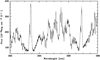 |
Fig. C.1 Ca II H& K lines of TYC 5340–1656–1. |
C.24 TYC 5340–1656–1
This star is classified as an RS CVn binary (stars with a giant primary of type F–K and a dwarf secondary of type G–M), in the Gaia DR3 catalogue. Our UVES spectrum shows two almost equally strong line systems, the cross correlation peaks provide the radial velocities provided in Table C.1. This fact clearly rules out the interpretation of this system as a classical RS CVn system since the two companions are of comparable luminosity. They are certainly giants, given the fact that the Balmer lines show no detectable wings. However it is interesting that both stars are chromospherically active (a typical signature of RS CVn systems) and this is obvious in Fig. C.1 where the core emissions of the Ca II H and K lines of both companions are clearly visible. A chemical analysis of such a star is beyond the scope of our paper, and in any case knowledge of the luminosity ratio of the two stars is required. By a quick comparison of the observed spectrum with synthetic spectra we expect the metallicity to be roughly solar and the v sin i of both stars between 20 and 30 km/s.
C.25 TYC 5422–1192–1
The star is a G giant member of the Open Cluster NGC 2423. The age of the cluster is estimated to be 310 Myr by (Bossini et al. 2019) and Dias et al. (2021) provide a metallicity of +0.12. Our UVES spectrum shows that the star is a fast rotator, probably above 100 km/s.
C.26 TYC 5763–1084–1
Analysed in the RVS range with the COOL grid, our UVES spectrum requires a shift of −1.2 kms−1 with respect to the Gaia radial velocity.
C.27 TYC 6108–150–1
According to the Gaia DR3 catalogue this star is an SB1 binary, with a period of 390.6 days and a semi-amplitude of 13.9 kms−1. The radial velocity of the centre of mass is 103.81 kms−1, almost 6 kms−1 from our adopted radial velocity. The eccentricity is very low 0.06.
C.28 TYC 6195–815–1
Gaia DR3 classifies this star as LPV with a period of 365.63 days and an amplitude of 0.09 mag. Analysed in the RVS range with the COOL grid, our UVES spectrum requires a shift of +2.2 kms−1 with respect to the Gaia radial velocity.
C.29 TYC 8400–1610–1
The effective temperature from the Mucciarelli et al. (2021) is 3748 K we run MyGIsFOS in the RVS range with the COOL grid and Teff= 3750 K to avoid extrapolation. Our UVES spectrum requires a shift of –2.3 kms−1 with respect to the Gaia radial velocity.
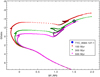 |
Fig. C.2 Position in the Gaia CMD of TYC 8584–127–1 compared to three BASTI isochrones with metallicity −0.40. |
Radial velocities for the components of SB2 stars.
C.30 TYC 8394–14–1
Gaia DR3 classifies this star as an LPV with a period of 603.23 days and an amplitude of 0.05 mag.
C.31 TYC 8584–127–1
This stars has a measurable rotational velocity, that suggests that it is a young evolved massive star, similar to those studied by Lombardo et al. (2021). From a fot to an isolated Fe I line we derive a projected rotational velocity of 11.5 kms−1. If we compare the position of the star in the CMD with BASTI isochrones (Pietrinferni et al. 2021) of metallicity −0.40 the implied age is 300 Myr and the mass 3.2 M⊙. The radial velocity measured from our blue UVES spectrum is 21.67 kms−1, in excellent agreement with the Gaia radial velocity (21.97 ± 0.23). Our radial velocity has not been zeroed on telluric lines so that the associated error is dominated by the centering of the star on the slit and this is of the order of 0.5 km−1.
We ran MyGIsFOS in the RVS range and found [Fe/H]=−0.58 ± 0.09 from 16 Fe I lines. It is remarkable to find that such a young star is shown to be moderately metal-poor. Its Galactic orbit is circular on the Galactic plane at roughly the solar radius.
References
- Alvarez, R., & Plez, B. 1998, A&A, 330, 1109 [NASA ADS] [Google Scholar]
- Arcones, A., & Thielemann, F.-K. 2023, A&AR, 31, 1 [NASA ADS] [CrossRef] [Google Scholar]
- Argast, D., Samland, M., Thielemann, F.-K., & Qian, Y.-Z. 2004, A&A, 416, 997 [NASA ADS] [CrossRef] [EDP Sciences] [Google Scholar]
- Bailer-Jones, C. A. L., Rybizki, J., Fouesneau, M., Demleitner, M., & Andrae, R. 2021, AJ, 161, 147 [Google Scholar]
- Barbá, R. H., Minniti, D., Geisler, D., et al. 2019, ApJ, 870, L24 [CrossRef] [Google Scholar]
- Barbuy, B., Cayrel, R., Spite, M., et al. 1997, A&A, 317, L63 [NASA ADS] [Google Scholar]
- Bayo, A., Rodrigo, C., Barrado Y Navascués, D., et al. 2008, A&A, 492, 277 [NASA ADS] [CrossRef] [EDP Sciences] [Google Scholar]
- Beers, T. C., & Christlieb, N. 2005, ARA&A, 43, 531 [NASA ADS] [CrossRef] [Google Scholar]
- Belokurov, V., Erkal, D., Evans, N. W., Koposov, S. E., & Deason, A. J. 2018, MNRAS, 478, 611 [Google Scholar]
- Bensby, T., Feltzing, S., & Oey, M. S. 2014, A&A, 562, A71 [NASA ADS] [CrossRef] [EDP Sciences] [Google Scholar]
- Bergemann, M., & Gehren, T. 2008, A&A, 492, 823 [NASA ADS] [CrossRef] [EDP Sciences] [Google Scholar]
- Bonifacio, P., Molaro, P., Beers, T. C., & Vladilo, G. 1998, A&A, 332, 672 [NASA ADS] [Google Scholar]
- Bonifacio, P., Spite, M., Cayrel, R., et al. 2009, A&A, 501, 519 [NASA ADS] [CrossRef] [EDP Sciences] [Google Scholar]
- Bonifacio, P., Monaco, L., Salvadori, S., et al. 2021, A&A, 651, A79 [NASA ADS] [CrossRef] [EDP Sciences] [Google Scholar]
- Bossini, D., Vallenari, A., Bragaglia, A., et al. 2019, A&A, 623, A108 [NASA ADS] [CrossRef] [EDP Sciences] [Google Scholar]
- Bovy, J. 2015, ApJS, 216, 29 [NASA ADS] [CrossRef] [Google Scholar]
- Bovy, J., Allende Prieto, C., Beers, T. C., et al. 2012, ApJ, 759, 131 [NASA ADS] [CrossRef] [Google Scholar]
- Burbidge, E. M., Burbidge, G. R., Fowler, W. A., & Hoyle, F. 1957, Rev. Mod. Phys., 29, 547 [NASA ADS] [CrossRef] [Google Scholar]
- Busso, M., Gallino, R., & Wasserburg, G. J. 1999, ARA&A, 37, 239 [Google Scholar]
- Caffau, E., Sbordone, L., Ludwig, H. G., Bonifacio, P., & Spite, M. 2010, Astron. Nachr., 331, 725 [NASA ADS] [CrossRef] [Google Scholar]
- Caffau, E., Bonifacio, P., François, P., et al. 2011, Nature, 477, 67 [NASA ADS] [CrossRef] [Google Scholar]
- Caffau, E., Bonifacio, P., Korotin, S. A., et al. 2021, A&A, 651, A20 [NASA ADS] [CrossRef] [EDP Sciences] [Google Scholar]
- Caffau, E., Katz, D., Gómez, A., et al. 2024, A&A, 683, A72 [NASA ADS] [CrossRef] [EDP Sciences] [Google Scholar]
- Carter, C., Conroy, C., Zaritsky, D., et al. 2021, ApJ, 908, 208 [NASA ADS] [CrossRef] [Google Scholar]
- Castelli, F., & Kurucz, R. L. 2003, in IAU Symposium, 210, Modelling of Stellar Atmospheres, eds. N. Piskunov, W. W. Weiss, & D. F. Gray, A20 [NASA ADS] [Google Scholar]
- Cavallo, L., Cescutti, G., & Matteucci, F. 2021, MNRAS, 503, 1 [CrossRef] [Google Scholar]
- Cayrel, R., Depagne, E., Spite, M., et al. 2004, A&A, 416, 1117 [NASA ADS] [CrossRef] [EDP Sciences] [Google Scholar]
- Cescutti, G. 2008, A&A, 481, 691 [NASA ADS] [CrossRef] [EDP Sciences] [Google Scholar]
- Cescutti, G., & Chiappini, C. 2014, A&A, 565, A51 [NASA ADS] [CrossRef] [EDP Sciences] [Google Scholar]
- Cescutti, G., & Kobayashi, C. 2017, A&A, 607, A23 [NASA ADS] [CrossRef] [EDP Sciences] [Google Scholar]
- Cescutti, G., Romano, D., Matteucci, F., Chiappini, C., & Hirschi, R. 2015, A&A, 577, A139 [NASA ADS] [CrossRef] [EDP Sciences] [Google Scholar]
- Cescutti, G., Bonifacio, P., Caffau, E., et al. 2022, A&A, 668, A168 [NASA ADS] [CrossRef] [EDP Sciences] [Google Scholar]
- Charbonnel, C., Lagarde, N., Jasniewicz, G., et al. 2020, A&A, 633, A34 [NASA ADS] [CrossRef] [EDP Sciences] [Google Scholar]
- Cohen, J. G., Christlieb, N., Qian, Y. Z., & Wasserburg, G. J. 2003, ApJ, 588, 1082 [Google Scholar]
- Contursi, G., de Laverny, P., Recio-Blanco, A., & Palicio, P. A. 2021, A&A, 654, A130 [NASA ADS] [CrossRef] [EDP Sciences] [Google Scholar]
- Côté, B., Fryer, C. L., Belczynski, K., et al. 2018, ApJ, 855, 99 [Google Scholar]
- Côté, B., Eichler, M., Arcones, A., et al. 2019, ApJ, 875, 106 [Google Scholar]
- Cowan, J. J., Sneden, C., Lawler, J. E., et al. 2021, Rev. Mod. Phys., 93, 015002 [Google Scholar]
- Cristallo, S., Piersanti, L., Straniero, O., et al. 2011, ApJS, 197, 17 [NASA ADS] [CrossRef] [Google Scholar]
- Dekker, H., D’Odorico, S., Kaufer, A., Delabre, B., & Kotzlowski, H. 2000, SPIE Conf. Ser., 4008, 534 [Google Scholar]
- Denissenkov, P. A., Herwig, F., Battino, U., et al. 2017, ApJ, 834, L10 [Google Scholar]
- Dias, W. S., Monteiro, H., Moitinho, A., et al. 2021, MNRAS, 504, 356 [NASA ADS] [CrossRef] [Google Scholar]
- Duffau, S., Caffau, E., Sbordone, L., et al. 2017, A&A, 604, A128 [NASA ADS] [CrossRef] [EDP Sciences] [Google Scholar]
- Eitner, P., Bergemann, M., Hansen, C. J., et al. 2020, A&A, 635, A38 [NASA ADS] [CrossRef] [EDP Sciences] [Google Scholar]
- Ekström, S., Georgy, C., Eggenberger, P., et al. 2012, A&A, 537, A146 [Google Scholar]
- Feuillet, D. K., Sahlholdt, C. L., Feltzing, S., & Casagrande, L. 2021, MNRAS, 508, 1489 [NASA ADS] [CrossRef] [Google Scholar]
- François, P., Depagne, E., Hill, V., et al. 2003, A&A, 403, 1105 [NASA ADS] [CrossRef] [EDP Sciences] [Google Scholar]
- François, P., Matteucci, F., Cayrel, R., et al. 2004, A&A, 421, 613 [NASA ADS] [CrossRef] [EDP Sciences] [Google Scholar]
- François, P., Depagne, E., Hill, V., et al. 2007, A&A, 476, 935 [Google Scholar]
- François, P., Cescutti, G., Bonifacio, P., et al. 2024, A&A, 686, A295 [NASA ADS] [CrossRef] [EDP Sciences] [Google Scholar]
- Frischknecht, U., Hirschi, R., Pignatari, M., et al. 2016, MNRAS, 456, 1803 [Google Scholar]
- Gaia Collaboration (Brown, A. G. A., et al.) 2021, A&A, 649, A1 [NASA ADS] [CrossRef] [EDP Sciences] [Google Scholar]
- Gaia Collaboration (Vallenari, A., et al.) 2023, A&A, 674, A1 [NASA ADS] [CrossRef] [EDP Sciences] [Google Scholar]
- Gallino, R., Arlandini, C., Busso, M., et al. 1998, ApJ, 497, 388 [Google Scholar]
- Green, G. M., Schlafly, E., Zucker, C., Speagle, J. S., & Finkbeiner, D. 2019, ApJ, 887, 93 [NASA ADS] [CrossRef] [Google Scholar]
- Hampel, M., Karakas, A. I., Stancliffe, R. J., Meyer, B. S., & Lugaro, M. 2019, ApJ, 887, 11 [Google Scholar]
- Hampel, M., Stancliffe, R. J., Lugaro, M., & Meyer, B. S. 2016, ApJ, 831, 171 [Google Scholar]
- Hansen, C. J., Primas, F., Hartman, H., et al. 2012, A&A, 545, A31 [NASA ADS] [CrossRef] [EDP Sciences] [Google Scholar]
- Hansen, C. J., Montes, F., & Arcones, A. 2014, ApJ, 797, 123 [NASA ADS] [CrossRef] [Google Scholar]
- Hansen, C. J., Koch, A., Mashonkina, L., et al. 2020, A&A, 643, A49 [NASA ADS] [CrossRef] [EDP Sciences] [Google Scholar]
- Haywood, M., Di Matteo, P., Lehnert, M. D., et al. 2018, ApJ, 863, 113 [Google Scholar]
- Helmi, A., Babusiaux, C., Koppelman, H. H., et al. 2018, Nature, 563, 85 [Google Scholar]
- Hill, V., Barbuy, B., Spite, M., et al. 2000, A&A, 353, 557 [NASA ADS] [Google Scholar]
- Iben, Icko, J. 1967, ApJ, 147, 624 [NASA ADS] [CrossRef] [Google Scholar]
- Ishigaki, M. N., Aoki, W., & Chiba, M. 2013, ApJ, 771, 67 [NASA ADS] [CrossRef] [Google Scholar]
- Karakas, A. I., & Lattanzio, J. C. 2014, PASA, 31, e030 [NASA ADS] [CrossRef] [Google Scholar]
- Kurucz, R. L. 2005, Mem. Soc. Astron. Ital. Suppl., 8, 14 [Google Scholar]
- Lane, J. M. M., Bovy, J., & Mackereth, J. T. 2022, MNRAS, 510, 5119 [NASA ADS] [CrossRef] [Google Scholar]
- Lind, K., Primas, F., Charbonnel, C., Grundahl, F., & Asplund, M. 2009, A&A, 503, 545 [NASA ADS] [CrossRef] [EDP Sciences] [Google Scholar]
- Lindegren, L., Bastian, U., Biermann, M., et al. 2021, A&A, 649, A4 [EDP Sciences] [Google Scholar]
- Lodders, K., Palme, H., & Gail, H. P. 2009, Landolt Börnstein, 4B, 712 [Google Scholar]
- Lombardo, L. 2023, in Memorie della Societa Astronomica Italiana, 94, 99 [NASA ADS] [Google Scholar]
- Lombardo, L., François, P., Bonifacio, P., et al. 2021, A&A, 656, A155 [NASA ADS] [CrossRef] [EDP Sciences] [Google Scholar]
- Lombardo, L., Bonifacio, P., François, P., et al. 2022, A&A, 665, A10 [NASA ADS] [CrossRef] [EDP Sciences] [Google Scholar]
- Magrini, L., Lagarde, N., Charbonnel, C., et al. 2021, A&A, 651, A84 [NASA ADS] [CrossRef] [EDP Sciences] [Google Scholar]
- Maíz Apellániz, J., Holgado, G., Pantaleoni González, M., & Caballero, J. A. 2023, A&A, 677, A137 [NASA ADS] [CrossRef] [EDP Sciences] [Google Scholar]
- Mashonkina, L. I., Belyaev, A. K., & Shi, J. R. 2016, Astron. Lett., 42, 366 [NASA ADS] [CrossRef] [Google Scholar]
- Mashonkina, L., Jablonka, P., Sitnova, T., Pakhomov, Y., & North, P. 2017, A&A, 608, A89 [NASA ADS] [CrossRef] [EDP Sciences] [Google Scholar]
- Matas Pinto, A. M., Spite, M., Caffau, E., et al. 2021, A&A, 654, A170 [NASA ADS] [CrossRef] [EDP Sciences] [Google Scholar]
- Meszaros, S., Dupree, A. K., & Szentgyorgyi, A. 2008, AJ, 135, 1117 [NASA ADS] [CrossRef] [Google Scholar]
- Mucciarelli, A., Salaris, M., & Bonifacio, P. 2012, MNRAS, 419, 2195 [NASA ADS] [CrossRef] [Google Scholar]
- Mucciarelli, A., Pancino, E., Lovisi, L., Ferraro, F. R., & Lapenna, E. 2013, GALA: Stellar atmospheric parameters and chemical abundances [Google Scholar]
- Mucciarelli, A., Bellazzini, M., & Massari, D. 2021, A&A, 653, A90 [NASA ADS] [CrossRef] [EDP Sciences] [Google Scholar]
- Mucciarelli, A., Monaco, L., Bonifacio, P., et al. 2022, A&A, 661, A153 [NASA ADS] [CrossRef] [EDP Sciences] [Google Scholar]
- Mucciarelli, A., Bonifacio, P., Monaco, L., Salaris, M., & Matteuzzi, M. 2024, A&A, 689, A89 [NASA ADS] [CrossRef] [EDP Sciences] [Google Scholar]
- Myeong, G. C., Vasiliev, E., Iorio, G., Evans, N. W., & Belokurov, V. 2019, MNRAS, 488, 1235 [Google Scholar]
- Nishimura, N., Takiwaki, T., & Thielemann, F.-K. 2015, ApJ, 810, 109 [Google Scholar]
- Nissen, P. E., Akerman, C., Asplund, M., et al. 2007, A&A, 469, 319 [NASA ADS] [CrossRef] [EDP Sciences] [Google Scholar]
- Norris, J. E., Ryan, S. G., & Beers, T. C. 1997, ApJ, 489, L169 [NASA ADS] [CrossRef] [Google Scholar]
- Pietrinferni, A., Hidalgo, S., Cassisi, S., et al. 2021, ApJ, 908, 102 [NASA ADS] [CrossRef] [Google Scholar]
- Planck Collaboration X. 2016, A&A, 594, A10 [NASA ADS] [CrossRef] [EDP Sciences] [Google Scholar]
- Plez, B. 2012, Turbospectrum: Code for spectral synthesis, Astrophysics Source Code Library [record ascl:1205.004] [Google Scholar]
- Price-Whelan, A. 2018, Adrn/Pyia: V0.2 [Google Scholar]
- Remy, Q., Grenier, I. A., Marshall, D. J., & Casandjian, J. M. 2018, A&A, 616, A71 [NASA ADS] [CrossRef] [EDP Sciences] [Google Scholar]
- Rizzuti, F., Cescutti, G., Matteucci, F., et al. 2021, MNRAS, 502, 2495 [NASA ADS] [CrossRef] [Google Scholar]
- Roederer, I. U., Cowan, J. J., Preston, G. W., et al. 2014, MNRAS, 445, 2970 [NASA ADS] [CrossRef] [Google Scholar]
- Sbordone, L., Caffau, E., Bonifacio, P., & Duffau, S. 2014, A&A, 564, A109 [NASA ADS] [CrossRef] [EDP Sciences] [Google Scholar]
- Schönrich, R., Binney, J., & Dehnen, W. 2010, MNRAS, 403, 1829 [NASA ADS] [CrossRef] [Google Scholar]
- Seitenzahl, I. R., Cescutti, G., Röpke, F. K., Ruiter, A. J., & Pakmor, R. 2013, A&A, 559, L5 [NASA ADS] [CrossRef] [EDP Sciences] [Google Scholar]
- Smith, G. H., & Dupree, A. K. 1988, AJ, 95, 1547 [NASA ADS] [CrossRef] [Google Scholar]
- Smith, V. V., & Lambert, D. L. 1984, PASP, 96, 226 [Google Scholar]
- Sneden, C., Preston, G. W., McWilliam, A., & Searle, L. 1994, ApJ, 431, L27 [NASA ADS] [CrossRef] [Google Scholar]
- Spite, F., & Spite, M. 1982, A&A, 115, 357 [NASA ADS] [Google Scholar]
- Thygesen, A. O., Sbordone, L., Ludwig, H. G., et al. 2016, A&A, 588, A66 [NASA ADS] [CrossRef] [EDP Sciences] [Google Scholar]
- Timmes, F. X., Woosley, S. E., & Weaver, T. A. 1995, ApJS, 98, 617 [NASA ADS] [CrossRef] [Google Scholar]
- Vergely, J. L., Lallement, R., & Cox, N. L. J. 2022, A&A, 664, A174 [NASA ADS] [CrossRef] [EDP Sciences] [Google Scholar]
- Villanova, S., Monaco, L., Geisler, D., et al. 2019, ApJ, 882, 174 [NASA ADS] [CrossRef] [Google Scholar]
- Watson, D., Hansen, C. J., Selsing, J., et al. 2019, Nature, 574, 497 [NASA ADS] [CrossRef] [Google Scholar]
- Woosley, S. E., & Weaver, T. A. 1995, ApJS, 101, 181 [Google Scholar]
- Yong, D., Roederer, I. U., Grundahl, F., et al. 2014, MNRAS, 441, 3396 [NASA ADS] [CrossRef] [Google Scholar]
Note: three stars display E> 0 in Fig.3, upper right panel. These stars are, however, on bound orbits. In fact, their space velocities are lower than the escape velocities at their distances. It is a known and documented feature that “galpy potentials do not necessarily approach zero at infinity”. This is indeed the case of MWPotential2014.
All Tables
Targets’ velocity components in galactocentric cylindrical coordinates (VR,VT,VZ), apocentric and pericentric distances (rap, rperi), orbital eccentricities (ecc.) and maximum height over the galactic plane (Zmax).
Total orbital energy (E), angular momentum (LZ), radial and vertical actions (JR, JZ) and classification (class, see bottom of the table) of the program stars.
Abundances and line-to-line dispersion (σ) of elements in their ionisation state in [X/H].
All Figures
|
Fig. 1 G0 versus (GBP − GRP)0 diagram of the sample. The stars exhibiting Hα emission are reported in red. The green star symbol is the Li-rich star. The CMD is superimposed to the 12 Gyr BASTI isochrones (Pietrinferni et al. 2021) with metallicities [Fe/H] = −1.0 (solid grey line) and [Fe/H] = −2.0 (dashed grey line). |
| In the text | |
|
Fig. 2 Top-left: galactocentric Cartesian height over the galactic plane Z vs. cylindrical galactocentric radius R. Top-middle: targets’ Galactocentric Cartesian Y vs. X coordinates. Top-right: maximum height over the galactic plane Zmax vs. apocentric distance rap. Bottom-left: pericentric distance rperi vs. rap. Bottom-middle: zoom-in of the top-right panel. The region above the line is forbidden. Bottom-right: zoom-in of the bottom-left panel. The stars with zero eccentricity lie on the line rperi =rap. Targets classified as belonging to the thin- (magenta) or thick-disk (cyan), thin-thick transition (blue), and halo (black) are presented as filled circles. Candidate GSE and Seq. stars are denoted with red squares and green diamonds, respectively. |
| In the text | |
|
Fig. 3 Top-left: Toomre diagram ( Top-middle: VT vs. VR. Top-right: orbital energy E vs. angular momentum LZ. Bottom-left: orbital eccentricity vs. LZ. Bottom-middle: |
| In the text | |
|
Fig. 4 Spectra of the Hα line of the stars exhibiting P-Cygni and/or inverse P-Cygni profile. |
| In the text | |
|
Fig. 5 A(Li) versus log g diagram for CD-28 10039 in comparison with literature data: Lind et al. (2009, grey), Mucciarelli et al. (2022, black), Mucciarelli et al. (2024, red). The blue lines are the Spite (A(Li) ∼ 2.2, Spite & Spite 1982) and RGB (A(Li) ∼ 1.1, Mucciarelli et al. 2012) plateaus. |
| In the text | |
|
Fig. 6 Comparison of the spectra of the Li-rich star CD-28 10039 (red) with that of CD-27 1605 (black) in different wavelength regions. From the top to bottom: Li doublet at 670.78 nm, reddest line of the Mg II triplet at 518.36 nm, Hα at 656.28 nm, and the reddest line of the Ca II triplet at 866.21 nm. |
| In the text | |
|
Fig. 7 Spectral energy distribution of CD-28 10039 obtained from the VOSA service. The model obtained with the parameters indicated in the toplabel is shown in blue. An apparent NUV excess has been detected from GALAX photometry. |
| In the text | |
|
Fig. 8 α-elements abundances measured in the MINCE III stars. Black and cyan points are Galactic stars belonging to the halo and thick-disk, respectively. Candidate Gaia–Sausage–Enceladus (red squares) and Seq. (green diamonds) stars are also shown. The results of Cescutti et al. (2022) for the same substructures in the MINCE I sample are reported with same colors and smaller symbols. The gray points are the results of Lombardo et al. (2022). |
| In the text | |
|
Fig. 9 [S/Fe] versus [Fe/H] LTE (left panel) and NLTE (right panel) diagrams of the MINCE sample, the MINCE I (Cescutti et al. 2022) sample is identified by smaller symbols. Colors and symbols are the same as in Figure 8. |
| In the text | |
|
Fig. 10 Light-odd elements abundances measured in the MINCE stars, the MINCE I sample (Cescutti et al. 2022) is identified by smaller symbols. Colors and symbols are the same as in Figure 8. |
| In the text | |
|
Fig. 11 Iron-peak elements abundances measured in the MINCE stars, the MINCE I sample (Cescutti et al. 2022) is identified by smaller symbols. Colors and symbols are the same as in Figure 8. |
| In the text | |
|
Fig. 12 Neutron capture elements abundances measured in the MINCE stars, the MINCE I sample (François et al. 2024) is identified by smaller symbols. Colors and symbols are the same as in Figure 8. The stars of the CERES survey analyzed by Lombardo et al. (2021); Lombardo (2023) are reported in gray. |
| In the text | |
|
Fig. 13 Abundance ratio of [Eu/Ba] as a function of [Ba/H] for MINCE stars. MW halo, Seq., and GSE stars are reported as black dots, green diamond symbols, and red square symbols, respectively. The results for MINCE I stars (François et al. 2024) are represented with same color and smaller symbols. The Li-rich star CD-28 10039 (green) and CD- 38 13823 (magenta) are highlighted with star symbols. We added the samples from Ishigaki et al. (2013) for comparison. |
| In the text | |
|
Fig. A.1 Comparison between the chemical abundances in MINCE I and III stars and the chemical evolution model for Mg, Ca, Si, Ti, Sc, Mn, Co, and Ni. Colors and symbols are the same as in Figure 8. |
| In the text | |
|
Fig. A.2 Comparison between the chemical abundances in MINCE I and III stars and the chemical evolution model for Zn, Rb, Sr, Y, Zr, Ba, La, Eu. Colors and symbols are the same as in Figure 8. |
| In the text | |
|
Fig. C.1 Ca II H& K lines of TYC 5340–1656–1. |
| In the text | |
|
Fig. C.2 Position in the Gaia CMD of TYC 8584–127–1 compared to three BASTI isochrones with metallicity −0.40. |
| In the text | |
Current usage metrics show cumulative count of Article Views (full-text article views including HTML views, PDF and ePub downloads, according to the available data) and Abstracts Views on Vision4Press platform.
Data correspond to usage on the plateform after 2015. The current usage metrics is available 48-96 hours after online publication and is updated daily on week days.
Initial download of the metrics may take a while.