| Issue |
A&A
Volume 695, March 2025
|
|
|---|---|---|
| Article Number | A166 | |
| Number of page(s) | 25 | |
| Section | Cosmology (including clusters of galaxies) | |
| DOI | https://doi.org/10.1051/0004-6361/202451779 | |
| Published online | 18 March 2025 | |
Discriminating between cosmological models using data-driven methods
1
Dipartimento di Fisica “E. Pancini”, Università degli Studi di Napoli “Federico II”, Complesso Univ. Monte S. Angelo, Via Cinthia 9, I-80126 Napoli, Italy
2
Scuola Superiore Meridionale, Largo S. Marcellino 10, I-80138 Napoli, Italy
3
Istituto Nazionale di Fisica Nucleare (INFN), Sez. di Napoli, Complesso Univ. Monte S. Angelo, Via Cinthia 9, I-80126 Napoli, Italy
4
INAF – Astronomical Observatory of Capodimonte, Via Moiariello 16, I-80131 Napoli, Italy
⋆ Corresponding author; This email address is being protected from spambots. You need JavaScript enabled to view it.
Received:
3
August
2024
Accepted:
15
February
2025
Abstract
Context. This study examines the Pantheon+SH0ES dataset using the standard Lambda cold dark matter (ΛCDM) model as a prior and applies machine learning to assess deviations. Rather than assuming discrepancies, we tested the models’ goodness of fit and explored whether the data allow alternative cosmological features.
Aims. The central goal is to evaluate the robustness of the ΛCDM model compared with other dark energy models, and to investigate whether there are deviations that might provide new cosmological insights. This study takes a data-driven approach, using traditional statistical methods and machine learning techniques.
Methods. Initially, we evaluated six dark energy models using traditional statistical methods such as Monte Carlo Markov chain (MCMC) and static or dynamic nested sampling to infer cosmological parameters. We then adopted a machine learning approach, developing a regression model to compute the distance modulus for each supernova and expanding the feature set to 74 statistical features. We used an ensemble of four models: multi-layer perceptron, k-nearest neighbours, random forest regressor, and gradient boosting. Cosmological parameters were estimated in four scenarios using MCMC and nested sampling, while feature selection techniques (random forest, Boruta, and the Shapley additive explanation) were applied in three.
Results. Traditional statistical analysis confirms that the ΛCDM model is robust, yielding expected parameter values. Other models show deviations, with the generalised and modified Chaplygin gas models performing poorly. In the machine learning analysis, feature selection techniques, particularly Boruta, significantly improve model performance. In particular, models initially considered weak (generalised or modified Chaplygin gas) show significant improvement after feature selection.
Conclusions. This study demonstrates the effectiveness of a data-driven approach to cosmological model evaluation. The ΛCDM model remains robust, while machine learning techniques, in particular feature selection, reveal potential improvements to alternative models that could be relevant for new observational campaigns, such as the recent Dark Energy Spectroscopic Instrument survey.
Key words: equation of state / methods: data analysis / supernovae: general / cosmological parameters / dark energy
© The Authors 2025
 Open Access article, published by EDP Sciences, under the terms of the Creative Commons Attribution License (https://creativecommons.org/licenses/by/4.0), which permits unrestricted use, distribution, and reproduction in any medium, provided the original work is properly cited.
This article is published in open access under the Subscribe to Open model. This email address is being protected from spambots. You need JavaScript enabled to view it. to support open access publication.
1. Introduction
At the turn of the 21st century, a significant breakthrough in our comprehension of the cosmos occurred thanks to two separate teams of cosmologists. The Supernova Cosmology Project (Perlmutter et al. 1999) and the High-Z Supernovae Search Team (Schmidt et al. 1998) inaugurated a new era of cosmic understanding. By studying far-off type Ia supernovae (SNeIa), they uncovered a Universe that was expanding at an accelerated pace. The groundbreaking discovery necessitated a re-evaluation of longstanding cosmic assumptions and triggered the development of new models. Most of them are related to the concept of dark energy (Peebles & Ratra 2003), a cosmic enigma hypothesised to account for the observed accelerated expansion (see Bamba et al. 2012 for a review). Einstein’s general relativity, when applied to cosmology sourced by baryonic matter and radiation, cannot explain such an accelerated dynamics. As a result, new hypotheses regarding dark energy (Basilakos & Plionis 2009) or extensions of general relativity (Capozziello & De Laurentis 2011) have become imperative. The Lambda cold dark matter (ΛCDM) model, which revisits Einstein’s original concept of a cosmological constant, has emerged as a strong contender for explaining accelerated dynamics (Ostriker & Vishniac 1986). This model has revived the repulsive gravitational impact of the cosmological constant as a credible means of explaining cosmic acceleration. In terms of particle physics, the cosmological constant, Λ, is representative of vacuum energy (Weinberg 1989). Thus, the quest for a mechanism yielding a small, observationally consistent value for the cosmological constant remains paramount. Distinguishing between the myriad dark energy models necessitates the establishment of observational constraints, often derived from phenomena such as SNeIa, cosmic microwave background (CMB) radiation, and large-scale structure observations. A key objective when dealing with dark energy is identifying any potential deviations in the value of the parameter
 (1)
(1)
where pde is the pressure of dark energy and ρde is its energy density, from its standard value of
 (2)
(2)
and to determine whether it aligns with the cosmological constant or diverges at some cosmic scale. Following the recent Dark Energy Spectroscopic Instrument (DESI) results, a number of studies have explored the evolving nature of dark energy. In particular, research has suggested that dark energy may not be a constant force, as originally thought, and may be evolving over time (Tada & Terada 2024; Orchard & Cárdenas 2024).
The present study is devoted to this issue. Our aim is to show that concurring dark energy cosmological models can be automatically discriminated by applying machine learning techniques to suitable samples of data. The paper consists of two interconnected yet distinct parts. The initial section focuses on Bayesian inference using sampling techniques, specifically Monte Carlo Markov chains (MCMC; Geyer 1992) and nested sampling (NS; Skilling 2004), applied to the original dataset.
MCMC is a versatile method that can be used to sample from any probability distribution. Its primary use is for sampling from hard-to-handle posterior distributions in Bayesian inference. In Bayesian estimation, computing the marginalised probability can be computationally expensive, especially for continuous distributions. The key advantage of MCMC is its ability to bypass the calculation of the normalisation constant. The general idea of the algorithm involves initiating a Markov chain with a random probability distribution over states. It gradually converges towards the desired probability distribution. The algorithm relies on a condition (the detailed balance sheet) to ensure that the stationary distribution of the Markov chain approximates the posterior probability distribution.
If this condition is satisfied, it guarantees that the stationary state of the Markov chain approximates the posterior distribution. Although MCMC is a complex method, it offers great flexibility, allowing efficient sampling in high-dimensional spaces and solving problems with large state spaces. However, it has a limitation: MCMC is poor at approximating probability distributions with multiple modes.
Nested sampling is a computational algorithm used to estimate evidence (a measure of how well a model fits the data) and infer posterior distributions in Bayesian analysis. Introduced by Skilling (2004), it is characterised by its ability to deal efficiently with high-dimensional parameter spaces, such as those found in cosmological studies. Rather than uniformly exploring the parameter space like MCMC, NS strategically selects points, called ‘live points’, which are progressively refined to focus on regions of higher likelihood, making it particularly effective for testing complex cosmological models such as the generalised and modified Chaplygin gas models.
Nested sampling is particularly useful in cosmological analyses where multi-mode likelihoods, such as those arising in dark energy model tests, pose a challenge to traditional MCMC. By focusing on regions of high likelihood, NS efficiently narrows the plausible parameter space, making it ideal for our study, where we are investigating competing dark energy models that could yield complex, multi-mode posterior distributions. This method allows us to compare the likelihood of each model while providing robust parameter estimates, particularly for Ωm and w, which directly influence our conclusions about the evolution of dark energy. Furthermore, it has a built-in self-tuning capability, allowing immediate application to new problems.
In our work we used two versions of NS: one with a fixed number of live points, called static nested sampling (SNS), and one with a varying number of live points during runtime, called dynamic nested sampling (DNS). Our analysis considered six dark energy parameterisations, each with different properties and free parameters. Rather than assuming a deviation from ΛCDM, we used a machine learning approach to compare these models and determine which best describes the data. The models considered are:
-
ΛCDM: The standard model.
-
Linear redshift (Huterer & Turner 2001; Weller & Albrecht 2002): This model proposes a linear relation between redshift and w. It is the simplest possible parameterisation.
-
Chevallier-Polarski-Linder (CPL; Chevallier & Polarski 2001; Linder 2008): A simple, but flexible and robust, parameterisation that tries to cover the overall time evolution of w.
-
Squared redshift (Barboza & Alcaniz 2008): This model proposes a squared relation between redshift and w and covers the Universe redshift regions where the CPL parameterisation fails.
-
Generalised Chaplygin gas (GCG; Bento et al. 2002): The GCG model is the first scenario we investigated in which dark matter and dark energy are unified.
-
Modified Chaplygin gas (MCG; Benaoum 2012): The MCG model is a modified version of the GCG model and has the largest number of free parameters among the models we studied, three.
This scheme allowed us to assess how well each model fits the observational data, providing insights into possible variations in the behaviour of dark energy without assuming the need for a new paradigm.
In the second section of this study, inspired by the work of D’Isanto et al. (2016) and the Feature Analysis for Time Series (FATS) public Python library (Nun et al. 2015), we computed additional statistics for each supernova (SN) and used three feature selection techniques to identify significant parameters from a final set of 70 features. As we will see, it is possible to analyse four different cases: a ‘base’ case where no feature selection is used; a case where the first 18 features selected by random forest are taken (Liaw & Wiener 2002); a case where the feature selection method used is the Boruta method (Kursa & Rudnicki 2011); and a last case where the first 18 features selected by Shapley Additive exPlanations (SHAP) are taken into account (Lundberg & Lee 2017). We then used an ensemble learning strategy to create a predictive model for the distance modulus based on the selected features. The models we used in the ensemble learning are the following:
-
Multi-layer perceptron (MLP; Rumelhart et al. 1986): A modern feed-forward artificial neural network consisting of fully connected neurons with a non-linear kind of activation function.
-
k-nearest neighbours (k-NN; Cover & Hart 1967): A non-parametric supervised learning method used for both classification and regression.
-
Random forest regressor (RFRegressor; Breiman 2001): An ensemble learning method for classification, regression, and other tasks that operates by constructing a multitude of decision trees at training time. For regression tasks, the mean or average prediction of the individual trees is returned.
-
Gradient boosting (Schapire 1990): A machine learning technique used in regression and classification tasks, among others. It gives a prediction model in the form of an ensemble of weak prediction models, that is, models that make very few assumptions about the data, which are typically simple decision trees (Quinlan 1986). When a decision tree is the weak learner, the resulting algorithm is a called gradient-boosted tree (Friedman 2001).
Subsequently, the new dataset, composed of original redshifts and predicted distance moduli, is subjected to the same sampling techniques used in the derivation of cosmological parameters.
The paper is structured as follows: Section 2 outlines the six dark energy models analysed. In Sect. 3 the dataset is presented. We describe the Pantheon+SH0ES compilation of Type Ia Supernovae and the new features that have been added. Section 4 focuses on the feature selection techniques used and the models implemented in our ensemble learning. In Sect. 5 the different sampling techniques are described in detail, with an explanation of the specifics of MCMC and NS for the inference of cosmological parameters. We conclude with a brief introduction to the information criteria used to evaluate the performance of the techniques. Section 6 presents the results of the study, showing the insights gained by implementing traditional Bayesian inference techniques as well as machine learning and sampling methods. Finally, in Sect. 7 we summarise our conclusions and present some perspectives.
2. Dark energy models
There are several proposed alternatives to the ΛCDM model, ranging from adding phenomenological dark energy terms to modifying the Hilbert-Einstein action or considering other geometrical invariants (Cai et al. 2016). To refine the model with dark energy evolving over time, a barotropic factor ω(z) = P/ρ dependent on z can be considered. This is the equation of state (EoS) of the given cosmological model. However, this approach has a crucial aspect: it is not possible to define ω(z) a priori; it must be reconstructed starting from observations. As stated in Dunsby & Luongo (2016), it is advantageous to express the barotropic factor in terms of cosmic time or, more appropriately, as a function of the scale factor or redshift. This choice is based on the idea that dark energy could evolve through a generic function over the history of the Universe. In this sense, the cosmographic analysis can greatly help in reconstructing the cosmic flow by the choice of suitable polynomials in the redshift z (see e.g. Demianski et al. 2012; Capozziello et al. 2018, 2020, 2021; Benetti & Capozziello 2019). A straightforward approach involves expanding ω as a Taylor series in redshift, z:
 (3)
(3)
However, opting for this expansion could pose challenges, as it may lead to a divergence in the EoS at higher redshifts. While certain models, such as the linear redshift and Chaplygin gas, have been challenged by past studies (Fabris et al. 2011), we deliberately included a diverse set of parameterisations. Our goal is to use machine learning techniques to evaluate their relative performance across the dataset, rather than presupposing their validity or exclusion. This approach allows for an unbiased assessment of different dark energy descriptions, including both commonly accepted and alternative models.
The following paragraphs present the six models studied in this paper.
2.1. ΛCDM
The ΛCDM model is the standard cosmological model, characterised by w = −1, with the Hubble function given by
 (4)
(4)
While ΛCDM provides an excellent fit to a wide range of observational data, it does not address certain fundamental issues, such as the cosmic coincidence problem or the fine-tuning of Λ.
2.2. Linear redshift parameterisation
The linear redshift model is one of the simplest extensions of the ΛCDM, introducing a redshift-dependent EoS for dark energy:
 (5)
(5)
where w0 and wa (sometimes written as wz) are constants, with w0 representing the present value of w(z). The model reduces to ΛCDM for w0 = −1 and wa = 0. The corresponding Hubble function is
 (6)
(6)
where Ωm is the matter density parameter and Ωx is the dark energy density. However, this parameterisation diverges at high redshifts, requiring strong constraints on wa in studies using high redshift data, such as CMB observations (Wang & Dai 2006).
2.3. Chevallier-Polarski-Linder (CPL) parameterisation
The CPL parameterisation introduces a smoothly varying EoS with two parameters characterising the present value (w0) and its evolution with time:
 (7)
(7)
The corresponding Hubble function is given by Escamilla-Rivera & Capozziello (2019)
 (8)
(8)
The CPL model is widely used because of its flexibility and robust behaviour in describing the evolution of dark energy.
2.4. Squared redshift parameterisation
The squared redshift parameterisation model provides an improvement over the CPL in regions where the latter cannot be reliably extended to describe the entire cosmic history. Its functional form is
 (9)
(9)
which remains well behaved as z → −1. The corresponding Hubble function is
 (10)
(10)
Overall, the squared redshift parameterisation has the advantage of remaining finite throughout the history of the Universe.
2.5. Unified dark energy fluid scenarios
As an extension of conventional cosmological scenarios, within the framework of a homogeneous and isotropic Universe, we assumed that the gravitational sector follows the standard formulation of general relativity, with minimal coupling to the matter sector. Furthermore, we assumed that the total energy content of the Universe consists of photons (γ), baryons (b), neutrinos (ν), and a unified dark fluid (UDF; XU; Cardone et al. 2004; Paul & Thakur 2013). This UDF is capable of exhibiting properties characteristic of dark energy, dark matter or an alternative cosmic fluid as the Universe expands. Consequently, the total energy density is denoted as ρi, where i = γ, b, ν, XU. Each fluid component obeys a continuity equation of the form
 (11)
(11)
Standard solutions give ρb ∝ a−3 and ργ, ν ∝ a−4. For the UDF we assume a constant adiabatic sound velocity cs and express the pressure as  , where cs and
  are positive constants (Escamilla-Rivera et al. 2020). This formulation allows the fluid to exhibit both barotropic and Λ-like behaviour, effectively unifying dark matter and dark energy, a phenomenon known as dark degeneracy. By integrating the continuity equation for the UDF, we obtain
 (12)
(12)
 (13)
(13)
where  and ρXU = ρ0 − ρΛ, where ρ0 is the present dark energy density. The dynamical EoS is given by
 (14)
(14)
To fully describe the behaviour of XU, we need to specify a particular functional form for pXU in terms of ρXU.
2.5.1. Generalised Chaplygin gas model
The GCG model characterises XU via the EoS
 (15)
(15)
where A and 0 ≤ α ≤ 1 are free parameters. The case α = 1 corresponds to the original Chaplygin gas model. Solving the continuity equation gives the evolution of the energy density:
![Mathematical equation: $$ \begin{aligned} \rho _{\mathrm{gcg}}(a) = \rho _{\mathrm{gcg},0} \left[b + (1 - b)a^{-3(1+\alpha )}\right]^{\frac{1}{1+\alpha }}, \end{aligned} $$](/articles/aa/full_html/2025/03/aa51779-24/aa51779-24-eq19.gif) (16)
(16)
where ρgcg, 0 is the current energy density and  . The corresponding dynamical EoS is
 (17)
(17)
This model describes an effective transition between dark matter and dark energy behaviour, with an intermediate regime when α = 1.
2.5.2. Modified Chaplygin gas model
The MCG model extends the GCG by introducing a linear term in the pressure-density relation:
 (18)
(18)
where A, b and α are real constants with 0 ≤ α ≤ 1. Setting A = 0 yields a perfect fluid with w = b, while b = 0 restores the GCG model. The standard Chaplygin gas model corresponds to α = 0. The evolution of the energy density follows
![Mathematical equation: $$ \begin{aligned} \rho _{\mathrm{mcg}}(a) = \rho _{\mathrm{mcg},0} \left[b_s + (1 - b_s)a^{-3(1+b)(1+\alpha )}\right]^{\frac{1}{1+\alpha }}, \end{aligned} $$](/articles/aa/full_html/2025/03/aa51779-24/aa51779-24-eq23.gif) (19)
(19)
where ρmcg, 0 is the current MCG energy density, and  . The corresponding EoS becomes
 (20)
(20)
As an extension of the GCG model, the MCG retains similar behaviour across different cosmological epochs. The Chaplygin gas framework provides a versatile approach to studying the interplay between dark matter and dark energy throughout cosmic history (Yang et al. 2019). The interactions between these components can further elucidate the expansion dynamics of the Universe (Piedipalumbo et al. 2023).
3. Dataset
As mentioned, the used dataset is the Pantheon+SH0ES of 1701 SNeIa coming from a compilation of 18 different surveys covering a redshift range up to 2.26. Among the 1701 objects in the dataset, 151 are duplicates, observed in multiple surveys, and 12 are pairs or triplets of SN sibling (i.e. SNe found in the same host galaxy).
The number of features provided by the Pantheon+SH0ES dataset is 45, excluding the ID of the SN, the ID of the survey used for that observation, and a binary variable to distinguish the SNe used in SH0ES from those not included. However, to increase the reliability of our model predictions and better capture the intrinsic variability of SNeIa, we expanded the feature set from the original 45 features provided by the Pantheon+SH0ES dataset to 71 (still excluding the previously cited features) by incorporating additional statistical descriptors from D’Isanto et al. (2016) and the FATS Python library. These additional features help account for observational uncertainties and intrinsic scatter in the SN measurements, improving our ability to discriminate between cosmological models, especially in scenarios where small variations in the distance modulus could be critical. More information on this statistical parameter space is provided in the appendix.
3.1. The Pantheon+SH0ES compilation
The Pantheon+SH0ES dataset consists of 1701 SNeIa from 18 different surveys, spanning a redshift range from 0.001 to 2.26. This wide range provides valuable insights into the evolution of dark energy over cosmic time. The detailed distance moduli of each SN in the dataset serve as critical measurements for constraining key cosmological parameters, such as the Hubble constant (H0), the matter density (Ωm), and the dark energy EoS parameter (w). This comprehensive dataset is particularly useful for testing different dark energy models and assessing their consistency with the standard ΛCDM model.
The theoretical distance modulus (μ) is related to the luminosity distance (dL) by the equation
 (21)
(21)
where dL is expressed in megaparsecs (Mpc). To account for systematic uncertainties, standard analyses include a nuisance parameter M, which represents the unknown offset corresponding to the absolute magnitude of the SNe and is degenerate with the value of H0.
Assuming a flat cosmological model, the luminosity distance is related to the comoving distance (D) as
 (22)
(22)
where c is the speed of light. The normalised Hubble function (H(z)/H0) is then computed by taking the inverse derivative of D(z) with respect to redshift:
 (23)
(23)
Here H0 is assumed to be a prior value for normalising D(z).
4. Methods
In our study we used three different feature selection techniques to identify significant parameters from a final set of 70 features. We analysed four different cases: a baseline scenario with no feature selection, a scenario using the first 18 features selected by random forest, a scenario using Boruta feature selection, and a scenario using the first 18 features selected by SHAP. We chose these methods because they provide interpretability in the feature selection process and are well suited to handling the non-linear relationships expected in SN data. Random forest and Boruta identify feature importance based on decision tree splits, while SHAP values provide a game-theoretic measure of each feature’s contribution to the model’s predictions. Other methods, such as principal component analysis, were not used because they transform features into linear combinations of the original variables, making it difficult to retain direct physical interpretability. Similarly, recursive feature elimination was not used because it selects features based on the performance of a particular model, which can introduce bias and limit generalisability across different learning algorithms.
We then used an ensemble learning approach to develop a predictive model for the distance modulus based on the selected features. The ensemble consists of four models: MLP, k-NN, RFRegressor, and gradient boosting. Each of these models brings unique capabilities to the ensemble, from the flexible architecture of MLP to the non-parametric nature of k-NN, the ensemble learning of random forest, and the gradient-boosted trees approach of gradient boosting.
We decided to use these models because they strike a balance between flexibility, interpretability and performance in a complex, non-linear problem. Gaussian processes were not used because they do not scale well with large datasets (such as Pantheon+SH0ES) due to their cubic complexity in training. Linear regression was considered, but is not well suited to capturing non-linear dependences in the data, making it a poor choice for modelling SN distance modules. The chosen ensemble approach exploits the strengths of several algorithms to improve robustness and generalisation.
4.1. Feature selection techniques
Feature selection is a crucial step in the process of building machine learning models, playing a pivotal role in enhancing model performance, interpretability, and efficiency. In many real-world scenarios, datasets often contain a multitude of features, and not all of them contribute equally to the predictive task at hand. Some features may even introduce noise or lead to computational inefficiencies.
4.1.1. Random forest
In the building of the single decision trees, the feature selected at each node is the one that minimises the chosen loss function (like the mean squared error in our case). Feature importance in a random forest is calculated based on how much each feature contributes to the reduction in loss function across all the trees in the ensemble. The more frequently a feature is used to split the data and the higher the loss function reduction it achieves, the more important it is considered. In random forests, ‘impurity’ refers to the degree of disorder or uncertainty in a decision tree. A ‘loss function’ quantifies this disorder and measures how well the model is performing. If a feature (such as the redshift or luminosity distance) reduces the impurity at multiple decision points within the tree ensemble, it is considered important (Liaw & Wiener 2002). This averaged reduction across all trees is used to assess the overall contribution of each feature in predicting cosmological parameters.
4.1.2. Boruta
The second method used is an all-relevant feature selection method, or Boruta. The Boruta algorithm takes its name from a demon in Slavic mythology who lived in pine forests and preyed on victims by walking like a shadow among the trees. And, in fact, main concept behind this method is the introduction of ‘shadow features’ and the use of random forest as predicting model (Kursa & Rudnicki 2011). A shadow feature for each real one is introduced by randomly shuffling its values among the N samples of the given dataset. It uses a random forest classifier, and so is a feature selection wrapping method, on this extended dataset (real and shadow features) and applies a feature importance measure such as the mean decrease accuracy and evaluates the importance of each feature. At every iteration, the Boruta algorithm checks whether a real feature has a higher importance than the best of its shadow features and constantly removes features that are deemed highly unimportant. Finally, the Boruta algorithm stops either when all features gets confirmed or rejected or it reaches a specified limit of iterations.
In conclusion, the steps of this algorithm can be summarised like this:
-
Take the original features and make a shuffled copy. The new extended dataset is now composed of the original features and their shuffled copy, the shadow features.
-
Run a random forest classifier on this new dataset and calculate the feature importance of every feature.
-
Store the highest feature importance of the shadow features and use it as a threshold value.
-
Keep the original features that have an importance higher than the highest shadow feature importance. We say that these features make a hit.
-
Repeat the previous steps for some iterations and keep track of the hits of the original features.
-
Label as ‘confirmed’ or ‘important’ the features that have a significantly high number of hits; as ‘rejected’ the ones that instead have a significantly low number of hits; and as ‘tentative’ the ones that fall in between.
The algorithm stops when all features have an established decision, or when a pre-set maximal number of iterations is reached.
4.1.3. SHAP
The final feature selection method used in our study was SHAP (Lundberg & Lee 2017). SHAP adopts a game-theoretic approach to explain the output of machine learning models, connecting optimal credit allocation with local explanations using classic Shapley values from game theory and their related extensions. SHAP serves as a set of software tools designed to enhance the explainability, interpretability, and transparency of predictive models for data scientists and end-users (Lundberg et al. 2020). SHAP is used to explain an existing model. In the context of a binary classification case built with a sklearn model, the process involves training, tuning, and testing the model. Subsequently, SHAP is employed to create an additional model that explains the classification model (see Figs. 1, 3 and 4).
The key components of a SHAP explanation include:
-
the explainer: the type of explainability algorithm chosen based on the model used.
-
the base value: the value that would be predicted if no features were known for the current output, typically the mean prediction for the training dataset or the background set (also called the reference value).
-
the Shapley values: the average contribution of each feature to each prediction for each sample based on all possible features. It is a (n, m) matrix (where n is the samples and m the features) that represents the contribution of each feature to each sample.
Explainers are the models used to calculate Shapley values. The diagram above (Fig. 2) shows different types of explainers. The choice of explainers depends mainly on the selected learning model. The kernel explainer creates a model that substitutes the closest to our model. It also can be used to explain neural networks. For deep learning models, there are the deep and gradient explainers. In our work we used a tree explainer. Shapley values calculate feature importance by evaluating what a model predicts with and without each feature. Since the order in which a model processes features can influence predictions, this comparison is performed in all possible ways to ensure fair assessments. This approach draws inspiration from game theory, and the resulting Shapley values facilitate the quantification of the impact of interactions between two features on predictions for each sample. As the Shapley values matrix has two dimensions (samples and features), interactions are represented as a tensor with three dimensions (samples, features, and features).
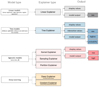 |
Fig. 2. Types of explainers (Czerwinska 2020). Panel a: Sum of a row of matrices (features by features) equals the SHAP value of this feature and this sample. Panel b: Diagonal entries equal the main effect of this feature on the prediction. Panel c: Symmetrical entries out of the diagonal equal the interaction effect between all the pairs of features for a given sample. |
 |
Fig. 3. SHAP matrix (Czerwinska 2020). |
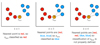 |
Fig. 4. k-NN classification. A simple solution for the last case is to randomly select one of the two classes or use an odd k (Nami 2021). |
4.2. Ensemble learning
From the plethora of different machine learning techniques available, the one used in this work is the ensemble learning. In this approach, two or more models are fitted on the same data and the predictions from each model are combined. The goal of ensemble learning is to achieve better performance with the ensemble of models than with each individual model by mitigating the weaknesses of each individual model. The models that compose the ensemble learning used in the work will be discussed in the following paragraphs.
4.2.1. Multi-layer perceptron
The MLP is the first of the four models used in the ensemble learning used in the work. The MLP is one of the most common used feed-forward neural network model (Van Der Malsburg 1986; Rumelhart et al. 1986; Brescia et al. 2015, 2019) and comes from the profound limitations of the first Rosenblatt perceptron in the treatment of non linearly separable, noisy and non numerical data. The term ‘feed-forward’ refers to the fact that in this neural network model, the impulse is always propagated in the same direction, for example from the input layer to the output layer, passing through one or more hidden layers, by combining the sum of weights associated with all neurons except the input ones. The output of each neuron is obtained by an activation function applied to the weighted sum of the inputs. The shape of the activation function can vary considerably from model to model, from the simplest linear function to the hyperbolic tangent, which is the one used in this work. In the training phase of the network, the weights are modified according to the learning rule used, until a predetermined distance between the network output and the desired output is reached (usually this distance is decided a priori by the user and is commonly known as the error threshold).
The easiest way to employ gradient information is to choose the weight update to make small steps in the direction of the negative gradient such that
 (24)
(24)
where the parameter η > 0 is referred to as the learning rate. In each iteration, the vector is adjusted in the direction of the steepest decrease of the error function, and this strategy is called gradient descent. We still need to define an efficient technique to find the gradient of the error function, E(w). A widely used method is the error back-propagation in which information is sent alternately forwards and backwards through the network. However, this method lacks precision and optimisation for complex real-life applications. Therefore, modifications are necessary.
Adaptive moment estimation (ADAM; Kingma & Ba 2014) takes a step forwards in the pursuit of the minimum of the objective function by solving the problem of learning rate selection and avoiding saddle points. ADAM computes adaptive learning rates for each parameter and maintains an exponentially decaying average of past gradients. This average is weighted with respect to the first two statistical moments of the gradient distribution. Adam behaves like a heavy ball with friction, where  and
and  are the estimate of the first and second moment of the gradients, and are computed as
 (25)
(25)
 (26)
(26)
where β1 and β2 are the characteristic memory times of the first and second moment of the gradients and control the decay of the moving averages. The final formula is then
 (27)
(27)
In summary, ADAM’s advantage lies in its use of the second moment of the gradient distribution. The hyperparameters used to build our MLP were two hidden layers with 100 neurons each, the tanh as the activation function, 1000 epochs, the initial learning rate set to 0.01, and ADAM as the optimisation technique.
4.2.2. k-nearest neighbours
The second model used in our work was the k-NN and it is a non-parametric supervised learning method used for both classification and regression. For regression problems, like our work, the k-NN works like this:
-
Choose a value for k: this determines the number of nearest neighbours used to make the prediction.
-
Calculate the distance: We calculated the distance between each data point in the training set and the target data point for which a prediction is made.
-
Find the k-NN: After calculating the distances, we identified the k-NN by selecting the k data points nearest to the new data point.
-
Calculate the prediction: After finding the k neighbours, we calculated the value of the dependent variable for the new data point. For this, we took the average of the target values of the k-NN. In most cases, the values of the points were weighted by the inverse of their distance.
For classification problems, a class label is assigned on the basis of a majority vote (i.e. the label that is most frequently represented around a given data point is used).
Three different algorithms are available to perform k-NN:
-
Brute force: We simply calculated the distance from the point of interest to all the points in the training set and took the class with most points.
-
k-dimensional tree (kd tree; Bentley 1975): A kd tree is a hierarchical binary tree. When this algorithm is used for k-NN classification, it rearranges the whole dataset in a binary tree structure, so that when test data are provided, it would give out the result by traversing through the tree, which takes less time than a brute search.
-
Ball tree (Bhatia 2010): is a hierarchical data structure similar to kd trees and is particularly efficient for higher dimensions.
The hyperparameters selected for constructing our k-NN model are determined using GridSearchCV (Grid Search Cross Validation) from the sklearn Python library (Pedregosa et al. 2011). This method identifies the optimal combination of hyperparameters from a predefined parameter grid based on a specified scoring function, with the negative mean squared error employed in our work. Additionally, GridSearchCV utilises cross-validation to refine the model parameters, and in our case, a cv value of 10 was applied. The ultimate hyperparameters are as follows:
-
the number of neighbours, the k value, is 4 when no feature selection is employed, 5 for feature selection with the random forest and Boruta, 6 when the feature selection is done with SHAP;
-
the weight is the inverse of the distance used;
-
the power parameter p for the Minkowski metric is 1, so we used the Manhattan distance;
-
the algorithm hyperparameter used to compute the nearest neighbours was left as ‘auto’, so that the model will automatically use the most appropriate algorithm based on the values passed to the fit method.
4.2.3. Random forest
The third model utilised in our study is RFRegressor. This model works by creating an ensemble of decision trees during the training phase, each based on different subsets of input data samples. Within the construction of each tree, various combinations of features inherent in data patterns are incorporated into the decision-making process. By employing a sufficient number of trees (dependent on the problem space complexity and input data volume), the produced forest is likely to represent all given features (Hastie et al. 2009). Regression models, in general sense, are able to take variable inputs and predict an output from a continuous range. In the context of regression models, which predict an output within a continuous range, decision tree regressions typically lack the ability to produce continuous output. Instead, they are trained on examples with output lying in a continuous range.
The hyperparameters used to build our RFRegressor model were the following:
-
The number of trees is 10 000.
-
The criterion to measure the quality of a split is the mean squared error.
-
The maximum depth of the trees is set to None, so the nodes are expanded until all leaves are pure or until all leaves contain fewer than min_samples_split samples.
-
The minimum number of samples required to split an internal node, the hyperparameter of the previous point min_samples_split, is set to 2.
-
The number of feature to consider when looking for the best split hyperparameter is set to auto, so that the max features to consider is equal to the number of features available.
4.2.4. Gradient boosting
The fourth and last model used in our work is the gradient boosting regressor (GBRegressor). In the previous paragraph we discuss the bagging technique; here we discuss the boosting technique, which is somewhat complementary. Boosting is a sequential type of ensemble learning that uses the result of the previous model as input for the next one. Instead of training the models separately, the upgrade trains the models in sequence, with each new model being trained to correct the errors of the previous ones. At each iteration the correctly predicted results are given a lower weight and those erroneously predicted a greater weight. It then uses a weighted average to produce a final result. Boosting is an iterative meta-algorithm that provides guidelines on how to connect a set of weak learners to create a strong learner. The key to the success of this paradigm lies in the iterative construction of strong learners, where each step involves introducing a weak learner tasked with ‘adjusting the shot’ based on the results obtained by its predecessors. Gradient boosting employs standard gradient descent to minimise the loss function used in the process. Typically, the weak learners are decision trees, and in this case, the algorithm is termed gradient-boosted trees.
The typical steps of a gradient boosting algorithm are the following:
-
The average of the target values is calculated for the initial predictions and the corresponding initial residual errors.
-
A model (shallow decision tree) is trained with independent variables and residual errors as data to obtain predictions.
-
The additive predictions and residual errors are calculated with a certain learning rate from the previous output predictions obtained from the model.
-
Steps 2 and 3 are repeated a number M of times until the required number of models are built.
-
The final boost prediction is the additive sum of all previous made by the models.
The hyperparameters used to build our GBRegressor were the following:
-
The loss function used is the squared error.
-
The learning rate, which defines the contribution of each tree, is set to 0.01.
-
The number of boosting stages is set to 10 000.
-
The function used to measure the quality of a split is the friedman_mse, or the mean squared error with the improvement by Friedman.
-
The minimum number of samples required to split an internal node is set to 2.
-
The maximum depth of the trees is set to None, so the nodes are expanded until all leaves are pure or until all leaves contain fewer than min_samples_split samples.
-
The number of feature to consider when looking for the best split hyperparameter is set to None, so that the max features to consider is equal to the number of features available.
5. Sampling techniques
This section introduces the techniques used in our work to perform cosmological parameters inference using the Pantheon+SH0ES SNIa dataset. The methods used in our project are MCMC and NS. MCMC is a probabilistic method that explores the parameter space by generating a sequence of samples, where each sample is a set of parameter values. The core of the method is related to the Markov property, which means that the next state in the sequence depends only on the current state (Norris 1998). In the context of cosmological parameter inference, MCMC is often used to sample the posterior distribution of parameters given observational data. It explores the parameter space by creating a chain of samples, with the density of samples reflecting the posterior distribution. Through analysis of this chain, one can estimate the most probable values and uncertainties for cosmological parameters. In our work we used two versions of NS: the standard version and the dynamic version, which is a slight variation of the former. Nested sampling is a technique used for Bayesian evidence calculation and parameter estimation and involves enclosing a shrinking region of high likelihood within the prior space and iteratively sampling points from this region. Nested sampling was developed to estimate the marginal likelihood, but it can also be used to generate posterior samples, and it can potentially work on harder problems where standard MCMC methods may get stuck. Dynamic nested sampling is an extension of NS that adapts the sampling strategy during the process. It starts with a high likelihood region and dynamically adjusts the sampling to focus on regions of interest. This method is advantageous for exploring complex and multi-mode parameter spaces, which can occur in cosmological models. At the end of each technique, we evaluated its performance by calculating the Bayesian information criterion (BIC; Schwarz 1978) and the Akaike information criterion (AIC; Akaike 1974).
5.1. Monte Carlo Markov chain
Bayesian inference treats probability as a measure of belief, with parameters treated as random variables influenced by data and prior knowledge. The goal is to combine prior information with observational data to refine our estimates and obtain a posterior distribution that summarises everything we know about the parameters (Bolstad 2009).
The posterior distribution is given by
 (28)
(28)
where P(D|Θ) is the likelihood, and π(Θ) is the prior. Since this distribution is often difficult to calculate analytically, MCMC provides a way to approximate it by generating a chain of parameter sets that converge to the posterior distribution over time. This allows us to estimate key cosmological parameters, even in high-dimensional spaces where standard methods struggle.
5.1.1. Markov chains
MCMC is based on the concept of a Markov chain, where each state depends only on the previous one (the so-called Markov property):
 (29)
(29)
The process is designed to ensure that the chain converges to the target posterior distribution after a number of steps. A key requirement is the detailed balance condition:
 (30)
(30)
This ensures that the chain remains in the desired distribution, allowing accurate parameter estimates.
5.1.2. The Metropolis-Hastings algorithm
The simplest and most commonly used MCMC algorithm is the Metropolis-Hastings method (Metropolis et al. 1953; MacKay 2003; Gregory 2005; Hogg et al. 2010). The iterative procedure is the following:
-
Given a position X(t), sample a proposal position Y from the transition distribution Q(Y; X(t)).
-
Accept this proposal with probability
 (31)
(31)
where D is a set of observations. If accepted, the new position will be X(t + 1) = Y; otherwise, it remains at X(t + 1) = X(t). This algorithm converges to a stationary distribution over time, but there are alternative methods that can achieve faster convergence depending on the problem.
5.1.3. The stretch move
The stretch move algorithm, proposed by Goodman & Weare (2010), is an affine-invariant method that outperforms the standard Metropolis-Hastings algorithm by producing independent samples with shorter autocorrelation times. It works by generating an ensemble of K walkers, where the proposal for a walker is based on the current positions of the others.
The new position for walker Xk is proposed using
![Mathematical equation: $$ \begin{aligned} X_k(t) \rightarrow Y = X_j + Z[X_k(t) - X_j], \end{aligned} $$](/articles/aa/full_html/2025/03/aa51779-24/aa51779-24-eq39.gif) (32)
(32)
where Z is a random variable. This method ensures a detailed balance and faster convergence, making it suitable for high-dimensional parameter spaces.
5.1.4. Our implementation of Monte Carlo Markov chain
In our work we applied MCMC to both the original dataset, which includes measured redshifts and distance modulus, and the predicted dataset, which includes measured redshift and predicted distance modulus obtained from our ensemble learning model. The hyperparameters used in our analysis are as follows:
-
The number of walkers is set to 100.
-
The move is the previously discussed StretchMove.
-
The number of steps varies: 1000 steps for the original dataset, and 2500 for the predicted dataset to account for the additional uncertainty of the machine learning models.
-
The number of initial steps of each chain discarded as burn-in is set to 100.
-
The initial positions of the walkers are randomly generated around the initial values for the cosmological parameters investigated with specified standard deviations (see Table 1).
Table 1.Initial conditions for MCMC.
5.2. Nested sampling
Modern astronomy often involves inferring physical models from large datasets. This has shifted the standard statistical framework from frequentist approaches such as maximum likelihood estimation (Fisher 1922) to Bayesian methods, which estimate the distribution of parameters consistent with the data and prior knowledge. While MCMC is widely used for Bayesian inference (Brooks et al. 2011; Sharma 2017), it can struggle with complex, multi-mode distributions and does not directly estimate the model evidence needed for model comparison (Plummer 2003; Foreman-Mackey et al. 2013; Carpenter et al. 2017).
Nested sampling (Skilling 2006) provides a solution by focusing on both posterior sampling and evidence estimation. It samples from nested regions of increasing likelihood, allowing more effective exploration of complex parameter spaces. The final set of samples, combined with their importance weights, helps generate posterior estimates while also providing a way to compute evidence for model comparison.
Unlike MCMC, which directly estimates the posterior P(Θ), NS decomposes the problem by:
-
splitting the posterior into simpler distributions;
-
sampling sequentially from each distribution;
-
and combining the results to estimate the overall posterior and evidence.
The goal is to compute the evidence, 𝒵, given by
 (33)
(33)
where ℒ(X) defines iso-likelihood contours outlining the prior volume X. This procedure allows NS to handle complex, high-dimensional problems that may be difficult for MCMC. Figure 5 illustrates the difference between MCMC methods and NS, where MCMC generates samples directly from the posterior, whereas NS breaks the posterior into nested slices, samples from each, and then combines them to reconstruct the original distribution with appropriate weights.
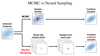 |
Fig. 5. While MCMC methods attempt to generate samples directly from the posterior, NS instead breaks up the posterior into many nested ‘slices’, generates samples from each of them, and then recombines the samples to reconstruct the original distribution using the appropriate weights (Speagle 2020). |
5.2.1. Stopping criterion
Nested sampling typically stops when the estimated remaining evidence is below a certain threshold (Keeton 2011; Higson et al. 2018). The stopping condition is
 (34)
(34)
where ϵ is a user-defined tolerance that indicates how much evidence remains to be integrated. In the Python library dynesty (Speagle 2020; Higson et al. 2019), this tolerance is typically set to 1%.
5.2.2. Evidence and posterior
Once the sampling is complete, the evidence, 𝒵, is estimated by numerical integration, typically using the trapezoidal rule:
![Mathematical equation: $$ \begin{aligned} \hat{\mathcal{Z} } = \sum _{i=1}^{N+K} \frac{1}{2} [\mathcal{L} (\Theta _{i-1}) + \mathcal{L} (\Theta _i)] \times (\hat{X}_{i-1} - \hat{X}_i). \end{aligned} $$](/articles/aa/full_html/2025/03/aa51779-24/aa51779-24-eq42.gif) (35)
(35)
The posterior P(Θ) is then calculated by weighting the samples based on their probabilities and the volume they represent.
5.2.3. Benefits and drawbacks of nested sampling
Nested sampling has several advantages over traditional MCMC methods:
-
It can estimate both the evidence, 𝒵, and the posterior, P(Θ), whereas MCMC generally focuses only on the posterior (Lartillot & Philippe 2006; Heavens et al. 2017).
-
It performs well with multi-mode distributions, which can be difficult for MCMC to handle.
-
The stopping criteria in NS are based on evidence estimation, providing a more natural endpoint than MCMC, which uses sample size-based criteria.
-
Nested sampling starts integrating the posterior from the prior, allowing it to explore the parameter space smoothly without having to wait for convergence, unlike MCMC (Gelman & Rubin 1992; Vehtari et al. 2021).
However, NS has limitations:
-
It often samples from uniform distributions, which can limit flexibility when dealing with more complex priors.
-
Runtime increases with the size of the prior, making it less efficient if the prior is large, but does not significantly affect the posterior.
-
The integration rate remains constant throughout the process, so it does not allow the prioritisation of the posterior over the evidence, even as the number of live points increases.
5.2.4. Bounding distributions
In NS, the current live points are used to estimate the shape and size of regions in parameter space, which helps guide sampling more efficiently. We used the multiple ellipsoids method, where:
-
A bounding ellipsoid is first constructed to enclose all live points.
-
K-means1 clustering is used to divide the points into clusters, with new ellipsoids constructed around each cluster.
-
This process continues iteratively until no further decomposition is required.
5.2.5. Sampling methods
After constructing a bounds distribution, dynesty proceeds to generate samples conditioned on those bounds. We utilised a uniform sampling method in our work. The general procedure for generating uniform samples from overlapping bounds is as follows (Feroz & Hobson 2008):
-
Select a boundary with a probability proportional to its volume.
-
Sampling a point uniformly from the selected boundary.
-
Accept the point with a probability inversely proportional to the number of overlapping boundaries.
This approach ensures that samples are drawn efficiently from the defined bounds, maximising the likelihood of finding points in high-probability regions of the parameter space.
5.2.6. Dynamic nested sampling
In Sect. 5.2.3 we identify three main limitations of standard NS: (1) the need for a prior transform, (2) increased running time for larger priors, and (3) a constant rate of posterior integration. While the first two are inherent to the NS method, the third limitation can be addressed by adjusting the number of live points during the run. This approach, known as DNS (Higson et al. 2019), allows the algorithm to focus more on either the posterior (P(Θ)) or the evidence (𝒵), providing flexibility that standard NS lacks.
The key idea is to increase the number of live points K in areas where more detail is needed and reduce it where faster exploration is sufficient. This makes it more efficient to deal with complex parameter spaces without sacrificing accuracy in posterior or evidence estimation.
The number of live points K(X) as a function of the prior volume X is guided by an importance function I(X), which determines how resources are allocated during sampling. In dynesty, this importance function is defined as
 (36)
(36)
where fP is the relative importance assigned to estimating the posterior.
The posterior importance, IP(X), is proportional to the probability density of the importance weight p(X), meaning more live points are allocated in regions with high posterior mass. On the other hand, evidence importance I𝒵 focuses on regions where there is uncertainty in integrating the posterior, ensuring accurate evidence estimation. By varying the number of live points based on these importance functions, DNS strikes a balance between efficient sampling and accurate evidence estimation, improving performance in complex scenarios.
5.2.7. Our implementation of static and dynamic nested sampling
As with the MCMC method, we applied static and DNS to both the original and predicted datasets. The hyperparameters used are the same for both sampling methods and are the following:
-
The number of live points varies: 1000 steps for the original, and 2500 for the predicted dataset to account for the additional uncertainty of the machine learning models.
-
The bounding distribution used is the multi ellipsoids.
-
The sampling method used is uniform.
-
The maximum number of iterations, as the number of likelihood evaluations, is set to no limit. Iterations will stop when the termination condition is reached.
-
The dlogz value, which sets the ϵ of the termination condition (Eq. 34), is set to 0.01.
5.3. Information criteria
We next considered two statistical criteria in order to compare our MCMC and NS results. The first, the AIC, is defined as
 (37)
(37)
where ℒ is the maximum likelihood and k is the number of parameters in the model. The optimal model is the one that minimises the AIC, since it provides an estimate of a constant plus the relative difference between the unknown true likelihood function of the trained sampler and the fitted likelihood function of the cosmological model. Therefore, a lower AIC indicates that the model is closer to the true underlying likelihood.
The second, the BIC, is defined as
 (38)
(38)
where N is the number of data points used in the fit. The BIC serves as an estimate of a function related to the posterior probability of a model being the true model within a Bayesian framework. Therefore, a lower BIC indicates that a model is deemed more likely to be the true model.
6. Results
As mentioned before, our work can be divided into two main sections: where we operated on the original SNe type Ia dataset, and where we used the predicted distance modulus dataset after feature selection methods and an ensemble model. In particular, as discussed earlier, we used three feature selection methods to build the predicted dataset:
-
Random forest: We took the 18 most important features of the total 70. The features considered are: m_b_corr, mB, zCMB, x0, zHEL, zHD, std_flux, m_b_corr_err_VPEC, MU_SH0ES_ERR_DIAG, m_b_corr_err_DIAG, skew, NDOF, percent_amplitude, DEC, biasCors_m_b_COVSCALE, fpr35, K, COV_c_x0.
-
Boruta: We took the confirmed features. The 13 accepted features employed are m_b_corr, mB, x0, zCMB, zHEL, zHD, std_flux, m_b_corr_err_VPEC, MU_SH0ES_ERR_DIAG, m_b_corr_err_DIAG, percent_amplitude, DEC, and MWEBV.
-
SHAP: As with the random forest, we took the 18 most important features: m_b_corr, mB, zCMB, x0, zHEL, zHD, std_flux, m_b_corr_err_VPEC, MU_SH0ES_ERR_DIAG, m_b_corr_err_DIAG, percent_amplitude, DEC, NDOF, biasCors_m_b_COVSCALE, fpr35, skew, RA, and COV_c_x0.
To summarise and highlight the differences between the three parameter spaces used, Fig. 6 below shows the random forest and SHAP importance, on a logarithmic scale, of the features selected by at least one of the techniques, together with the Boruta classification.
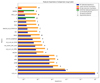 |
Fig. 6. Feature importance comparison. Dark blue bars show the importance of features selected by the random forest model, and dark orange bars the importance of features selected by SHAP. Red bars represent the importance of features not selected by the random forest model, and green bars the importance of features not selected by SHAP. The symbols indicate the Boruta classification: + for confirmed, | for tentative, and x for rejected features. More information on all features (Pantheon+SH0ES dataset and additions) can be found in the appendix. |
We also performed a ‘base’ case study where all 70 features were used to predict distance moduli with an ensemble model. After each MCMC and NS iteration, BIC and AIC have been computed. The final cosmological parameters and their uncertainties have been obtained as the mean of the three methods used. This work is developed for all the previously introduced six cosmological models, thanks to the Astropy Python package (Price-Whelan et al. 2022). A summary of the results is provided in the appendix. This includes corner plots obtained by each technique and a table showing the key results, such as BIC and AIC scores, for each method.
In Figs. 7–15 we indicate the original dataset with ‘OR’, the case where no feature selection is done with ‘ALL’ (i.e. all features are used), the case where random forest is used as feature selection technique with ‘RF’, the case where the Boruta technique is used with ‘BOR’, and the case where SHAP is used as feature selection method with ‘SHAP’. In addition, ‘MCMC’, ‘SNS’, and ‘DNS’ indicate the different sampling techniques.
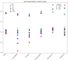 |
Fig. 7. Hubble constant values. |
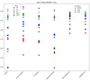 |
Fig. 8. Matter density values. |
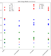 |
Fig. 9. w (w0) values. |
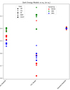 |
Fig. 10. wa (wz) values. |
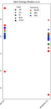 |
Fig. 11. b values. |
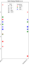 |
Fig. 12. α values. |
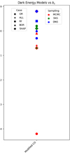 |
Fig. 13. bs values. |
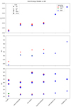 |
Fig. 14. BIC values. |
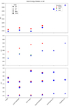 |
Fig. 15. AIC values. |
Figure 7 shows the derived values of the Hubble constant H0 for each cosmological model under different feature selection methods. The plot contrasts the results obtained from the original dataset with those obtained using feature selection techniques along with different sampling techniques such as MCMC, SNS, and DNS. In particular, the results from the original dataset tend to be higher compared to all other values found in the second part. The opposite trend is seen in Fig. 8, which compares the matter density parameter. The results show significant deviations when no feature selection is applied, emphasising the importance of selecting relevant features to avoid skewed or biased estimates. In addition, the GCG and MCG models show a different behaviour compared to other models, with generally higher values, further emphasising their divergence from standard cosmological models. In the Fig. 9, where the evolution of the EoS parameter w0 is shown for the different models, the values seem to be related to the particular sampling technique used, with the exception of the case where no feature selection was applied, which is an alarming sign for its performance. Furthermore, Fig. 10 presents the analysis of the EoS parameter wa (or wz). A notable finding is that the linear and squared redshift models give more or less the same results, while the CPL model covers a much wider range of values. In addition, Figs. 11–13 show the parameters specific to the Chaplygin gas models, b, α, and bs, respectively.
From Figs. 14 and 15, which respectively show the values of BIC and AIC for the analysed models, we can draw some interesting conclusions. Firstly, the values of BIC and AIC are much higher in the original dataset with respect to the other four cases, but this is due to the difference in the size of the dataset used, complete for the first scenario and 20% for the others, which leads to much larger penalty terms in the final values of the Information Criteria. Secondly, among the scenarios of the second part of the study, the case where no feature selection has been applied, has the highest values in BIC and AIC, which is representative of the fact that this is the worst case analysed, because not only we do not obtain a better performance, but we also have the higher complexity in the model. Among the three cases analysed, Boruta clearly has the lowest Information Criteria values and therefore the better sampling performance. Looking at the models, it is interesting to note that from the original dataset scenario to those where the feature selection has been applied, the Chaplygin gas models have the greatest increase in performance compared to the other models. Finally, remaining in the three cases of feature selection, the model that has the lowest mean values of BIC and AIC is the linear redshift one, but this may be due to the low redshift of our dataset, which favours this model.
7. Discussion and conclusions
In this work we tested six dark energy models with recent observations of SNeIa. First, we tested each model by inferring its cosmological parameters using MCMC, SNS, and DNS. Secondly, we tried a different approach using machine learning. We built a regression model where the distance modulus of each SN, the crucial data for inferring the cosmological parameters, was computed by the machine learning model, thanks to the other available features. We relied on the features provided by the original dataset (Scolnic et al. 2022) but also extended it by several features, bringing the total number to 74. The machine learning model used to compute the distance moduli is an ensemble model composed of four models: the MLP, the k-NN, the RFRegressor, and the gradient boosting model. To improve the performance of our ensemble learning model, we applied different feature selection techniques, emphasising the importance of a data-driven approach. We inferred the cosmological parameters of each model in four different cases: a case where no feature selection is applied (a sort of ‘base’ case), a case where the first 18 features selected by the random forest are used to infer the distance moduli, a case where the feature selection method used is Boruta, and finally a case where the features used are the first 18 selected by SHAP. For every case, we repeated the process done in the first part of the study, or used MCMC and NS, to infer the cosmological parameters for each model. By incorporating feature selection methods, we ensured that our models focused on the most relevant and informative features, thereby improving the robustness of the distance modulus predictions.
In the first phase of our study, the ΛCDM parameters were found to be consistent with established observations, confirming its status as a robust standard cosmological model. While the introduction of new parameters in the linear, squared redshift, and CPL models led to slight deviations, the overall parameter values remained relatively similar across the different parameterisations. On the other hand, the GCG and MCG models showed significant deviations, especially in the matter density parameter, making them the worst performing of the six models.
Moving to the second part of our work, it is important to point out the results of the feature selection processes. The analysis shows that the most important feature by a significant margin is m_b_corr, which represents the Tripp1998 corrected mb magnitude. Following at some distance are mB (SALT2 uncorrected brightness; Guy et al. 2007) and x0 (SALT2 light curve amplitude). Next in importance are zCMB, zHEL, and zHD, corresponding to the CMB-corrected redshift, the heliocentric redshift, and the Hubble diagram redshift, respectively. The remaining features are of lesser importance, and their contributions are roughly comparable to one another. It is worth noting that the selected features are predominantly from the original dataset, with only a few additions made by us, such as std_flux, percent_amplitude, skew, fpr35, and K. This highlights the robustness of the original dataset features in influencing the predictive power of our models. However, our inclusion of additional features has provided valuable insights and contributed to the overall effectiveness of the feature selection process.
In the second section of our work, the first result we noticed is the clear difference in the performance of the ensemble model between the case where no feature selection is applied and the three cases where it is. In the former, the parameters differ significantly from the values found in the first part of the work; additionally, the values of the information criteria, BIC and AIC, are almost two times the values of the cases where feature selection is applied. The performances observed for the three feature selection models are quite similar, following a similar trend as in the first part of the study. In particular, by looking at the values of the most important cosmological parameters, the GCG and MCG models appear to be slightly less effective than the other four. Of the random forest, Boruta, and SHAP models, the random forest seems to perform slightly worse, and the other two show comparable results. Furthermore, our analysis reveals an interesting aspect in the estimation of the wa (or wz) parameter across the dark energy models. The linear and squared redshift parameterisation models give similar estimates, while the CPL model shows a larger variation. In general, the trend across all six models indicates a slightly lower H0 and a slightly higher Ωm compared to the values obtained in the first part of the study. It is worth noting that Boruta stands out as the model with the lowest information criterion values. It is interesting to note that when looking at the BIC and AIC values, for the models that seemed to be by far the worst in the first part of the study (i.e. the GCG and MCG models), in the case where no feature selection is applied, a poor result is only found for the MCG, while GCG is among the best models. On the other hand, for the three cases of feature selection, the opposite is true, with the GCG model behaving similarly to the CPL and squared redshift models and the MCG model performing the best of the four. In summary, the feature selection models, especially Boruta, show consistent performance with variations in H0 and Ωm. The unexpected ranking of the information criteria of the models, which challenges conventional expectations based on theoretical considerations, adds an interesting dimension to the overall interpretation. This highlights the importance of a data-driven approach to cosmological studies, where feature selection can lead to more nuanced insights into dark energy models.
In the future, we aim to extend our investigation using the cosmological constraints provided by DESI. The recent DESI Data Release 1 (Adame et al. 2025) provides robust measurements of Baryon acoustic oscillations (BAOs) in several tracers, including galaxies, quasars, and Lyman-α forests, over a wide redshift range from 0.1 to 4.2. These measurements provide valuable insights into the expansion history of the Universe and place stringent constraints on cosmological parameters. The implications of the DESI BAO measurements are of particular interest for the nature of dark energy. The DESI data, in combination with other cosmological probes such as the Planck measurements of the CMB and the SNIa datasets, may provide new perspectives on the EoS parameter of dark energy (w) and its possible time evolution (w0 and wa). The discrepancy between the DESI BAO data and the standard ΛCDM model, especially in the context of the dark energy EoS, opens up avenues for further investigation. By incorporating the DESI BAO measurements into our analysis framework, we expect to refine our understanding of the dark energy dynamics and its implications for the overall cosmic evolution. In addition, recent results (Colgáin et al. 2024) show that a ∼2σ discrepancy with the PlanckΛCDM cosmology in the DESI luminous red galaxy data at zeff = 0.51 leads to an unexpectedly large Ωm value,  . This anomaly causes the preference for w0 > −1 in the DESI data when confronted with the w0waCDM model. Independent analyses confirm this anomaly and show that DESI data allow Ωm to vary by of the order of ∼2σ with increasing effective redshift in the ΛCDM model. Given the tension between luminous red galaxy data at zeff = 0.51 and SNeIa at overlapping redshifts, the statistical significance of this anomaly is expected decrease in future DESI data releases, although an increasing Ωm trend with effective redshift may persist at higher redshifts.
Recent works (Alfano et al. 2024; Luongo & Muccino 2024; Sapone & Nesseris 2024; Carloni et al. 2025) have tested the DESI results, in particular with respect to possible systematic biases in the BAO constraints and their compatibility with the ΛCDM model. While some analyses highlight tensions in the derived values of Ωm and the dark energy EoS (w), others argue that these discrepancies are due to systematic uncertainties rather than a fundamental departure from ΛCDM. Our approach does not aim to directly challenge or confirm these tensions, but instead provides a complementary, data-driven methodology for testing dark energy models using SNe.
The main novelty of our work lies in the application of advanced feature selection and machine learning techniques to extract meaningful information from SN datasets. Rather than assuming a specific parametric form for the evolution of dark energy, our method enables a more flexible, data-driven exploration of cosmological constraints. While our results are broadly consistent with ΛCDM, our approach provides an independent validation of existing results while highlighting the role of statistical methods in cosmology. Future incorporation of DESI data into our framework will further test whether the observed anomalies persist when analysed using our methodology.
It is worth noting that these results are not based on theoretical assumptions but are derived directly from the data through our data-driven approach. By employing several feature selection techniques, we allow the data to guide our exploration of dark energy models. Building on these results, future research will incorporate DESI observations to further refine and develop more reliable constraints on dark energy models.
K-means is a clustering algorithm that categorises data into K clusters by iteratively assigning data points to the cluster with the closest centroid, aiming to minimise the variance within each cluster. This process continues until convergence, resulting in K clusters with centroids that represent the centre of each cluster’s data points.
Acknowledgments
This article is based upon work from COST Action CA21136 Addressing observational tensions in cosmology with systematic and fundamental physics (CosmoVerse) supported by COST (European Cooperation in Science and Technology). SC acknowledges the support of Istituto Nazionale di Fisica Nucleare (INFN), iniziative specifiche MoonLight2 and QGSKY. MB acknowledges the ASI-INAF TI agreement, 2018-23-HH.0 “Attivitá scientifica per la missione Euclid – fase D”. The dataset used in this study is openly accessible and can be found at https://pantheonplussh0es.github.io/. Additionally, the data is available in the public version of SNANA within the directory labeled “Pantheon+”. The full SNANA dataset is archived on Zenodo and can be downloaded from https://zenodo.org/record/4015325 and the SNANA source directory is https://github.com/RickKessler/SNANA
References
- Adame, A. G., Aguilar, J., Ahlen, S., et al. 2025, JCAP, 02, 021 [CrossRef] [Google Scholar]
- Akaike, H. 1974, IEEE Trans. Autom. Control., 19, 716 [NASA ADS] [CrossRef] [Google Scholar]
- Alfano, A. C., Luongo, O., & Muccino, M. 2024, JCAP, 2024, 055 [CrossRef] [Google Scholar]
- Bamba, K., Capozziello, S., Nojiri, S., & Odintsov, S. D. 2012, Ap&SS, 342, 155 [NASA ADS] [CrossRef] [Google Scholar]
- Barboza, E., & Alcaniz, J. 2008, Phys. Rev. Lett. B, 666, 415 [Google Scholar]
- Basilakos, S., & Plionis, M. 2009, A&A, 507, 47 [NASA ADS] [CrossRef] [EDP Sciences] [Google Scholar]
- Benaoum, H. B. 2012, Adv. High Energy Phys., 2012, 357802 [Google Scholar]
- Benetti, M., & Capozziello, S. 2019, JCAP, 12, 008 [CrossRef] [Google Scholar]
- Bentley, J. L. 1975, Commun. ACM, 18, 509 [CrossRef] [Google Scholar]
- Bento, M., Bertolami, O., & Sen, A. A. 2002, Phys. Rev. D, 66, 043507 [CrossRef] [Google Scholar]
- Bhatia, N. 2010, Int. J. Com. Sci. Inf. Sec., 8, 302 [Google Scholar]
- Bolstad, W. M. 2009, Understanding Computational Bayesian Statistics (John Wiley& Sons), 644 [CrossRef] [Google Scholar]
- Breiman, L. 2001, Mach. Learn., 45, 5 [Google Scholar]
- Brescia, M., Cavuoti, S., & Longo, G. 2015, MNRAS, 450, 3893 [NASA ADS] [CrossRef] [Google Scholar]
- Brescia, M., Salvato, M., Cavuoti, S., et al. 2019, MNRAS, 489, 663 [NASA ADS] [CrossRef] [Google Scholar]
- Brockwell, P. J., & Davis, R. A. 2002, Introduction to Time Series and Forecasting (Springer) [CrossRef] [Google Scholar]
- Brooks, S., Gelman, A., Jones, G., & Meng, X.-L. 2011, Handbook of Markov Chain Monte Carlo (CRC Press) [CrossRef] [Google Scholar]
- Cai, Y.-F., Capozziello, S., De Laurentis, M., & Saridakis, E. N. 2016, Rep. Prog. Phys., 79, 106901 [Google Scholar]
- Capozziello, S., & De Laurentis, M. 2011, Phys. Rep., 509, 167 [CrossRef] [Google Scholar]
- Capozziello, S., D’Agostino, R., & Luongo, O. 2018, MNRAS, 476, 3924 [NASA ADS] [CrossRef] [Google Scholar]
- Capozziello, S., D’Agostino, R., & Luongo, O. 2020, MNRAS, 494, 2576 [NASA ADS] [CrossRef] [Google Scholar]
- Capozziello, S., Dunsby, P. K. S., & Luongo, O. 2021, MNRAS, 509, 5399 [NASA ADS] [CrossRef] [Google Scholar]
- Cardone, V. F., Troisi, A., & Capozziello, S. 2004, Phys. Rev. D, 69, 083517 [Google Scholar]
- Carloni, Y., Luongo, O., & Muccino, M. 2025, Phys. Rev. D, 111, 023512 [Google Scholar]
- Carpenter, B., Gelman, A., Hoffman, M. D., et al. 2017, J. Stat. Softw., 76, 1 [NASA ADS] [CrossRef] [Google Scholar]
- Chevallier, M., & Polarski, D. 2001, Int. J. Mod. Phys. D, 10, 213 [Google Scholar]
- Colgáin, E. Ó., Dainotti, M. G., Capozziello, S., et al. 2024, ArXiv e-prints [arXiv:2404.08633] [Google Scholar]
- Cover, T., & Hart, P. 1967, IEEE Trans. Inf. Theory, 13, 21 [CrossRef] [Google Scholar]
- Czerwinska, U. 2020, Push the Limits of Explainability – an Ultimate Guide to SHAP Library, https://urszulaczerwinska.github.io/works/interpretability-shap [Google Scholar]
- Demianski, M., Piedipalumbo, E., Rubano, C., & Scudellaro, P. 2012, MNRAS, 426, 1396 [Google Scholar]
- D’Isanto, A., Cavuoti, S., Brescia, M., et al. 2016, MNRAS, 457, 3119 [CrossRef] [Google Scholar]
- Dunsby, P. K., & Luongo, O. 2016, Int. J. Geom. Meth. Mod. Phys., 13, 1630002 [NASA ADS] [CrossRef] [Google Scholar]
- Escamilla-Rivera, C., & Capozziello, S. 2019, Int. J. Mod. Phys. D, 28, 1950154 [NASA ADS] [CrossRef] [Google Scholar]
- Escamilla-Rivera, C., Quintero, M. A. C., & Capozziello, S. 2020, JCAP, 2020, 008 [CrossRef] [Google Scholar]
- Fabris, J. C., Velten, H. E. S., Ogouyandjou, C., & Tossa, J. 2011, Phys. Rev. Lett. B, 694, 289 [Google Scholar]
- Falk, M., Marohn, F., Michel, R., et al. 2011, A First Course on Time Series Analysis: Examples with SAS (epubli GmbH) [Google Scholar]
- Feroz, F., & Hobson, M. P. 2008, MNRAS, 384, 449 [NASA ADS] [CrossRef] [Google Scholar]
- Fisher, R. A. 1922, Phil. Trans. R. Soc. A, 222, 309 [Google Scholar]
- Foreman-Mackey, D., Hogg, D. W., Lang, D., & Goodman, J. 2013, PASP, 125, 306 [Google Scholar]
- Friedman, J. H. 2001, Ann. Stat., 29, 1189 [Google Scholar]
- Gelman, A., & Rubin, D. B. 1992, Stat. Sci., 7, 457 [Google Scholar]
- Geyer, C. J. 1992, Stat. Sci., 7, 473 [Google Scholar]
- Goodman, J., & Weare, J. 2010, Commun. App. Math. Comp. Sci., 5, 65 [NASA ADS] [CrossRef] [Google Scholar]
- Gregory, P. 2005, Bayesian Logical Data Analysis for the Physical Sciences: A Comparative Approach with Mathematica Support (Cambridge: Cambridge University Press) [CrossRef] [Google Scholar]
- Guy, J., Astier, P., Baumont, S., et al. 2007, A&A, 466, 11 [NASA ADS] [CrossRef] [EDP Sciences] [Google Scholar]
- Hastie, T., Tibshirani, R., Friedman, J., et al. 2009, The Elements of Statistical Learning: Data Mining, Inference and Prediction (Springer) [Google Scholar]
- Heavens, A., Fantaye, Y., Mootoovaloo, A., et al. 2017, ArXiv e-prints [arXiv:1704.03472] [Google Scholar]
- Higson, E., Handley, W., Hobson, M., & Lasenby, A. 2018, Bayesian Anal., 13, 873 [NASA ADS] [CrossRef] [Google Scholar]
- Higson, E., Handley, W., Hobson, M., & Lasenby, A. 2019, Stat. Comput., 29, 891 [Google Scholar]
- Hogg, D. W., Bovy, J., & Lang, D. 2010, ArXiv e-prints [arXiv:1008.4686] [Google Scholar]
- Huterer, D., & Turner, M. S. 2001, Phys. Rev. D, 64, 123527 [Google Scholar]
- Keeton, C. R. 2011, MNRAS, 414, 1418 [Google Scholar]
- Kingma, D. P., & Ba, J. 2014, ArXiv e-prints [arXiv:1412.6980] [Google Scholar]
- Kursa, M. B., & Rudnicki, W. R. 2011, ArXiv e-prints [arXiv:1106.5112] [Google Scholar]
- Lartillot, N., & Philippe, H. 2006, Syst. Biol., 55, 195 [Google Scholar]
- Li, Q. 2019, Shap-shapley, https://github.com/shaoshanglqy/shap-shapley [Google Scholar]
- Liaw, A., & Wiener, M. 2002, R News, 2, 18 [Google Scholar]
- Linder, E. V. 2008, Gen. Relativ. Gravit., 40, 329 [CrossRef] [Google Scholar]
- Lomb, N. R. 1976, Astrophys. Space Sci., 39, 447 [Google Scholar]
- Lundberg, S. M., & Lee, S.-I. 2017, Adv. Neural. Inf. Process. Syst., 30, 4768 [Google Scholar]
- Lundberg, S. M., Erion, G., Chen, H., et al. 2020, Nat. Mach. Intell., 2, 56 [CrossRef] [Google Scholar]
- Luongo, O., & Muccino, M. 2024, A&A, 690, A40 [NASA ADS] [CrossRef] [EDP Sciences] [Google Scholar]
- MacKay, D. J. 2003, Information Theory, Inference and Learning Algorithms (Cambridge: Cambridge University Press) [Google Scholar]
- Metropolis, N., Rosenbluth, A. W., Rosenbluth, M. N., Teller, A. H., & Teller, E. 1953, J. Chem. Phys., 21, 1087 [Google Scholar]
- Nami, Y. 2021, Why Does Increasing k Decrease Variance in kNN?, https://towardsdatascience.com/why-does-increasing-k-decrease-variance-in-knn-9ed6de2f5061 [Google Scholar]
- Norris, J. R. 1998, Markov Chains (Cambridge: Cambridge University Press) [Google Scholar]
- Nun, I., Protopapas, P., Sim, B., et al. 2015, ArXiv e-prints [arXiv:1506.00010] [Google Scholar]
- Orchard, L., & Cárdenas, V. H. 2024, Phys. Dark Univ., 46, 101678 [Google Scholar]
- Ostriker, J. P., & Vishniac, E. T. 1986, ApJ, 306, L51 [Google Scholar]
- Paul, B., & Thakur, P. 2013, J. Cosmol. Astropart. Phys., 2013, 052 [CrossRef] [Google Scholar]
- Pedregosa, F., Varoquaux, G., Gramfort, A., et al. 2011, J. Mach. Learn. Res., 12, 2825 [Google Scholar]
- Peebles, P. J. E., & Ratra, B. 2003, Rev. Mod. Phys., 75, 559 [NASA ADS] [CrossRef] [Google Scholar]
- Perlmutter, S., Aldering, G., Goldhaber, G., et al. 1999, ApJ, 517, 565 [Google Scholar]
- Piedipalumbo, E., Vignolo, S., Feola, P., & Capozziello, S. 2023, Phys. Dark Univ., 42, 101274 [Google Scholar]
- Plummer, M. 2003, Proceedings of the 3rd International Workshop on Distributed Statistical Computing, Vienna, Austria, 124, 1 [Google Scholar]
- Price-Whelan, A. M., Lim, P. L., Earl, N., et al. 2022, ApJ, 935, 167 [NASA ADS] [CrossRef] [Google Scholar]
- Quinlan, J. R. 1986, Mach. Learn., 1, 81 [Google Scholar]
- Rumelhart, D. E., Hinton, G. E., & Williams, R. J. 1986, Nature, 323, 533 [Google Scholar]
- Sapone, D., & Nesseris, S. 2024, ArXiv e-prints [arXiv:2412.01740] [Google Scholar]
- Scargle, J. D. 1982, ApJ, 263, 835 [Google Scholar]
- Schapire, R. E. 1990, Mach. Learn., 5, 197 [Google Scholar]
- Schmidt, B. P., Suntzeff, N. B., Phillips, M., et al. 1998, ApJ, 507, 46 [NASA ADS] [CrossRef] [Google Scholar]
- Schwarz, G. 1978, Ann. Stat., 6, 461 [Google Scholar]
- Scolnic, D., Brout, D., Carr, A., et al. 2022, ApJ, 938, 113 [NASA ADS] [CrossRef] [Google Scholar]
- Sharma, S. 2017, ARA&A, 55, 213 [Google Scholar]
- Skilling, J. 2004, AIP Conf. Proc., 735, 395 [Google Scholar]
- Skilling, J. 2006, Bayesian Anal., 1, 833 [Google Scholar]
- Speagle, J. S. 2020, MNRAS, 493, 3132 [Google Scholar]
- Stetson, P. B. 1996, PASP, 108, 851 [NASA ADS] [CrossRef] [Google Scholar]
- Tada, Y., & Terada, T. 2024, Phys. Rev. D, 109, L121305 [CrossRef] [Google Scholar]
- Van Der Malsburg, C. 1986, Brain Theory: Proceedings of the First Trieste Meeting on Brain Theory, October 1–4, 1984 (Springer), 245 [Google Scholar]
- Vehtari, A., Gelman, A., Simpson, D., Carpenter, B., & Bürkner, P.-C. 2021, Bayesian Anal., 16, 667 [CrossRef] [Google Scholar]
- Wang, F.-Y., & Dai, Z.-G. 2006, Chin. Astron. Astrophys., 6, 561 [CrossRef] [Google Scholar]
- Weinberg, S. 1989, Rev. Mod. Phys., 61, 1 [NASA ADS] [CrossRef] [Google Scholar]
- Weller, J., & Albrecht, A. 2002, Phys. Rev. D, 65, 103512 [Google Scholar]
- Yang, W., Pan, S., Vagnozzi, S., et al. 2019, JCAP, 11, 044 [CrossRef] [Google Scholar]
Appendix A: Pantheon+SH0ES features
The total number of features provided by the dataset is 48 and are described in the Table A.1.
Pantheon+SH0ES features.
Appendix B: Additional features
In our work we added more features to those already present in the Pantheon+SH0ES dataset in order to gain more confidence in the upcoming results. The total number of features is 74, and here we present the ones we added.
Amplitude (ampl)
The arithmetic average between the maximum and minimum magnitude is
 (B.1)
(B.1)
Beyond1std (b1std)
The fraction of photometric points above or under a certain standard deviation from the weighted average (by photometric errors) is
 (B.2)
(B.2)
Flux percentage ratio (fpr)
The percentile is the value of a variable under which there is a certain percentage of light curve data points. The flux percentile Fn, m was defined as the difference between the flux values at percentiles n and m. The following flux percentile ratios were used:
 (B.3)
(B.3)
 (B.4)
(B.4)
 (B.5)
(B.5)
 (B.6)
(B.6)
 (B.7)
(B.7)
Lomb-Scargle periodogram
The Lomb-Scargle periodogram (Lomb 1976; Scargle 1982) is a method for finding periodic signals in irregularly sampled time series data. It handles irregularly spaced observations, calculates the power spectral density at different frequencies and uses least squares fitting. The statistic used in our work is the period given by the peak frequency of the Lomb-Scargle periodogram.
Linear trend (slope)
The linear trend is the slope of the light curve in the linear fit, that is to say, the a parameter in the following linear relation:
 (B.8)
(B.8)
 (B.9)
(B.9)
Median absolute deviation (mad)
The median of the deviation of fluxes from the median flux is
 (B.10)
Median buffer range percentage (mbrp)
The fraction of data points that are within 10 percent of the median flux is
 (B.11)
Magnitude ratio (mr)
An index used to estimate if the object spends most of the time above or below the median of magnitudes is
 (B.12)
Maximum slope (ms)
The maximum difference obtained measuring magnitudes at successive epochs is
 (B.13)
Percent amplitude (pa)
The maximum percentage difference between maximum or minimum flux and the median is
 (B.14)
Percent difference flux percentile (pdfp)
This is difference between the second and the 98th percentile flux, converted in magnitudes. It is calculated by the ratio F5, 95 on median flux:
 (B.15)
Pair slope trend (pst)
The percentage of the last 30 couples of consecutive measures of fluxes that show a positive slope is
 (B.16)
R Cor Bor (rcb)
The fraction of magnitudes that is below 1.5 mag with respect to the median is
 (B.17)
Small kurtosis (sk)
The kurtosis represents the departure of a distribution from normality and it is given by the ratio between the fourth-order momentum and the square of the variance. For small kurtosis, it is intended the reliable kurtosis on a small number of epochs:
 (B.18)
Skew
The skewness is an index of the asymmetry of a distribution. It is given by the ratio between the third-order momentum and the variance to the third power:
 (B.19)
Standard deviation
This is the standard deviation of the fluxes.
Range of a cumulative sum (Rcs)
The range of a cumulative sum defined as
 (B.20)
 (B.21)
where l = 1, 2, …, N.
Stetson K (K)
A robust kurtosis measure (Stetson 1996) is defined as
 (B.22)
 (B.23)
Q3 − 1
This is the difference between the third and first quartile of the magnitude.
Mean variance (mvar)
This is a simple variability index defined as
 (B.24)
CAR features (σC, τ, andmean)
To model irregularly sampled time series, the continuous autoregressive (CAR) process, as presented in Brockwell & Davis (2002) and Falk et al. (2011), is employed. This continuous-time auto-regressive model involves three parameters and offers a natural and consistent means to estimate the characteristic timescale and variance of light curves. The CAR process is defined by the stochastic differential equation:
 (B.25)
where (τ, σC, t ≥ 0). The mean value of the light curve X(t) is bτ, and the variance is τσC2/2. Here, τ is the relaxation time, interpreting the variability amplitude of the time series, and σC describes variability on timescales shorter than τ. ϵ(t) is a white noise process with zero mean and unit variance.
The likelihood function for such a CAR model, considering light curve observations {x1, …, xn} at times {t1, …, tn} with measurement error variances {δ12, …, δn2}, is given by
 (B.26)
where xi* = xi − bτ,  , Ω0 = τσC2/2, and xi and Ωi are given by
 (B.27)
The parameter optimisation involves maximising the likelihood with respect to σC and τ, and b is determined as the mean magnitude of the light curve divided by τ.
Appendix C: Importance of XAI
Explainable artificial intelligence (XAI) plays a crucial role in improving the interpretability of machine learning models, especially in scientific applications where transparency is essential. In this appendix we highlight the importance of XAI using the SHAP framework and present a beeswarm plot (Fig. C.1) illustrating feature importances.
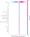 |
Fig. C.1. Beeswarm plot of the 20 most important features. |
Explanatory AI methods such as SHAP provide insight into the decision-making process of complex models, fostering confidence and facilitating the identification of potential biases or errors. By quantifying the impact of each feature on model predictions, SHAP scores provide a comprehensive understanding of feature importance while maintaining desirable properties such as consistency and local accuracy.
To visually represent feature importance, we present a beeswarm plot showing the distribution of SHAP values for the 20 most important features. This plot provides an intuitive visualisation of the relative impact of different variables on the model’s predictions, facilitating the identification of key predictors and supporting informed decision making in scientific analyses.
Appendix D: Additional results
A summary of the results for the ΛCDM and CPL models is given for both the original dataset and the Boruta cases. For brevity, only the results for these specific models and cases are included in this section. The priors have been chosen on the basis of physical considerations and existing literature to ensure numerical stability while allowing meaningful parameter exploration. Some contours may appear truncated, reflecting strong constraints imposed by the data rather than artificial priors.
 |
Fig. D.1. ΛCDM model corner plots for the original dataset: MCMC (a), SNS (b), and DNS (c). |
 |
Fig. D.2. CPL model corner plots for the original dataset: MCMC (a), SNS (b), and DNS. |
 |
Fig. D.3. ΛCDM model corner plots with Boruta features: MCMC (a), SNS (b), and DNS. |
 |
Fig. D.4. CPL model with Boruta features:MCMC (a), SNS (b), and DNS. |
ΛCDM model parameter values for the original dataset.
CPL model parameter values for the original dataset.
ΛCDM parameter values with Boruta features.
CPL parameter values with Boruta features.
All Tables
All Figures
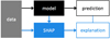 |
Fig. 1. SHAP architecture (Li 2019). |
| In the text | |
|
Fig. 2. Types of explainers (Czerwinska 2020). Panel a: Sum of a row of matrices (features by features) equals the SHAP value of this feature and this sample. Panel b: Diagonal entries equal the main effect of this feature on the prediction. Panel c: Symmetrical entries out of the diagonal equal the interaction effect between all the pairs of features for a given sample. |
| In the text | |
|
Fig. 3. SHAP matrix (Czerwinska 2020). |
| In the text | |
|
Fig. 4. k-NN classification. A simple solution for the last case is to randomly select one of the two classes or use an odd k (Nami 2021). |
| In the text | |
|
Fig. 5. While MCMC methods attempt to generate samples directly from the posterior, NS instead breaks up the posterior into many nested ‘slices’, generates samples from each of them, and then recombines the samples to reconstruct the original distribution using the appropriate weights (Speagle 2020). |
| In the text | |
|
Fig. 6. Feature importance comparison. Dark blue bars show the importance of features selected by the random forest model, and dark orange bars the importance of features selected by SHAP. Red bars represent the importance of features not selected by the random forest model, and green bars the importance of features not selected by SHAP. The symbols indicate the Boruta classification: + for confirmed, | for tentative, and x for rejected features. More information on all features (Pantheon+SH0ES dataset and additions) can be found in the appendix. |
| In the text | |
|
Fig. 7. Hubble constant values. |
| In the text | |
|
Fig. 8. Matter density values. |
| In the text | |
|
Fig. 9. w (w0) values. |
| In the text | |
|
Fig. 10. wa (wz) values. |
| In the text | |
|
Fig. 11. b values. |
| In the text | |
|
Fig. 12. α values. |
| In the text | |
|
Fig. 13. bs values. |
| In the text | |
|
Fig. 14. BIC values. |
| In the text | |
|
Fig. 15. AIC values. |
| In the text | |
|
Fig. C.1. Beeswarm plot of the 20 most important features. |
| In the text | |
|
Fig. D.1. ΛCDM model corner plots for the original dataset: MCMC (a), SNS (b), and DNS (c). |
| In the text | |
|
Fig. D.2. CPL model corner plots for the original dataset: MCMC (a), SNS (b), and DNS. |
| In the text | |
|
Fig. D.3. ΛCDM model corner plots with Boruta features: MCMC (a), SNS (b), and DNS. |
| In the text | |
|
Fig. D.4. CPL model with Boruta features:MCMC (a), SNS (b), and DNS. |
| In the text | |
Current usage metrics show cumulative count of Article Views (full-text article views including HTML views, PDF and ePub downloads, according to the available data) and Abstracts Views on Vision4Press platform.
Data correspond to usage on the plateform after 2015. The current usage metrics is available 48-96 hours after online publication and is updated daily on week days.
Initial download of the metrics may take a while.