| Issue |
A&A
Volume 694, February 2025
|
|
|---|---|---|
| Article Number | A196 | |
| Number of page(s) | 15 | |
| Section | Extragalactic astronomy | |
| DOI | https://doi.org/10.1051/0004-6361/202451894 | |
| Published online | 14 February 2025 | |
Investigating the redshift evolution of lensing galaxy density slopes via model-independent distance ratios
1
National Centre for Nuclear Research, ul. Pasteura 7, 02-093 Warsaw, Poland
2
Astronomical Observatory of the Jagiellonian University, Faculty of Physics, Astronomy and Applied Computer Science, ul. Orla 171, 30-244 Kraków, Poland
⋆ Corresponding authors; This email address is being protected from spambots. You need JavaScript enabled to view it.
; This email address is being protected from spambots. You need JavaScript enabled to view it.
; This email address is being protected from spambots. You need JavaScript enabled to view it.
Received:
15
August
2024
Accepted:
31
December
2024
Abstract
Context. Strong-lensing systems are expected to be discovered in great numbers by next-generation surveys. They provide a powerful tool for studying cosmology and the galaxy evolution. The coupling of the galaxy structure and cosmology through distance ratios means that it is essential for advancing both fields to examine the evolution of the lensing galaxy mass density profiles.
Aims. We introduce a novel method that is independent of the dark energy assumed in the model to investigate the mass density slopes of lensing galaxies and their redshift evolution using an extended power-law (EPL) model.
Methods. We adopted a nonparametric approach based on artificial neural networks trained on type Ia supernovae data to reconstruct the distance ratios of strong-lensing systems. These reconstructed ratios were compared with theoretical predictions to estimate the evolution of EPL model parameters.
Results. A negative evolutionary trend of the mass density power-law exponent with increasing redshift is observed across different analysis levels. Assuming a triangular prior for the anisotropy of lensing galaxies, we find evidence for a redshift evolution of the mass density slope, quantified as ∂γ/∂z = −0.20 ± 0.12.
Conclusions. This study confirms that the redshift evolution of the matter density slopes in lensing galaxies can be determined independent of dark energy models at the population level. The Legacy Survey of Space and Time (LSST) Rubin Observatory forecasts are expected to identify 100 000 strongly lensed galaxies. We show based on simulations with data from the LSST that spectroscopic follow up of just 10% of these systems can reduce the uncertainty in the redshift evolution coefficient of the total mass density slope (Δ∂γ/∂z) to 0.021. This precision would be able to distinguish between evolving and nonevolving scenarios for lensing galaxies.
Key words: gravitational lensing: strong / galaxies: evolution
© The Authors 2025
 Open Access article, published by EDP Sciences, under the terms of the Creative Commons Attribution License (https://creativecommons.org/licenses/by/4.0), which permits unrestricted use, distribution, and reproduction in any medium, provided the original work is properly cited.
This article is published in open access under the Subscribe to Open model. This email address is being protected from spambots. You need JavaScript enabled to view it. to support open access publication.
1. Introduction
Despite its limitations, the Λ cold dark matter (ΛCDM) model remains the standard paradigm for describing the Universe at the largest scales. Various well-established cosmological probes have been used within this framework to constrain the cosmological parameters. These probes encompass a wide range of techniques, including observations of the cosmic microwave background (CMB) (Planck Collaboration VI 2020), baryon acoustic oscillations (BAO) (Eisenstein et al. 2005; Cole et al. 2005; DESI Collaboration 2024), and supernovae Ia (SNIa) (Riess et al. 1998; Perlmutter et al. 1999; Riess et al. 2022). Moreover, alternative approaches using strong gravitational lenses (SGLs) (Suyu et al. 2014; Cao et al. 2015; Arendse et al. 2019; Liu et al. 2019; Liao et al. 2019, 2020; Wong et al. 2020; Qi et al. 2021; Li et al. 2024) and gravitational waves (Abbott et al. 2017; Gayathri et al. 2020) are being used complementary to the above methods. However, statistically significant discrepancies are observed between the results obtained from these various methods. This is commonly referred to as the Hubble tension (Di Valentino et al. 2021) and the S8 tension (Asgari et al. 2021; Harnois-Déraps et al. 2024). For a detailed discussion of cosmological tensions, we refer to Di Valentino et al. (2021). The authors highlighted the need for a further exploration and refinement of observational techniques (including a study of possible systematics and biases) and cosmological theories.
As a particularly valuable cosmological probe, SGL can provide independent constraints on cosmological parameters. Rooted in the theory of general relativity (GR), SGL describes the deflection of light from a distant source by the gravitational field of a massive intervening object. This phenomenon offers unique information about the link between the structure of galaxies and cosmological information, which makes it a powerful tool for studying cosmological parameters and galaxy evolution.
A key observable in studies of SGLs is the position and shape distortion of lensed images, which can be obtained with high-resolution data. This information allows us to determine the Einstein radius θE. This quantity represents the angular radius of the ring-like image that forms when light from a perfectly aligned background source is bent by the gravity of lensing galaxies. θE provides a robust measurement of the total projected mass of the lensing object. Furthermore, when combined with stellar kinematics data, it can help us to constrain the radial mass profile of the lens (Treu & Koopmans 2002; Koopmans & Treu 2003; Koopmans 2006). However, the observed angular size of the Einstein radius depends on the cosmological model, as it is influenced by the distances between the source, lens, and observer; specifically, via the distance ratio DlsA/DsA, where DlsA is the angular diameter distance from the lens to the source, and DsA is the angular diameter distance from the source to the observer. The dependence mentioned above means that the Einstein radius is a valuable observable for testing cosmological models, provided there is an accurate lens model for comparison with theoretical predictions. This approach was employed in testing dark energy models (Cao et al. 2011, 2012a) and cosmic curvature (Liu et al. 2020; Wang et al. 2022), and to constrain cosmological models (Biesiada et al. 2010; Cao et al. 2012b, 2015).
One of the prerequisites in the approaches mentioned above is an assumption about the mass profile of the lensing galaxy. We use the extended power-law (EPL) model here, where power-law density profiles describe both luminous and dark matter. Allowing for different radial density distributions between the luminous and dark matter components provides us the freedom to describe the mass distribution of the lensing galaxy in a more realistic way. The EPL model was developed by Koopmans (2006), and it provides an analytical solution that enhances the computational efficiency. It was therefore broadly used in various applications. These include the constraint of cosmological parameters (Chen et al. 2019; Li et al. 2024), the exploration of the Friedmann-Lemaître-Robertson-Walker (FLRW) metric (Cao et al. 2019; Wang et al. 2022), a test of theories of general relativity (Lian et al. 2022; Guerrini & Mörtsell 2024), the examination of dark matter models (Bora et al. 2021; Cheng et al. 2021), and the study of galaxy evolution (Geng et al. 2021).
The question now is whether the EPL model is adequate for a statistical analysis of SGL samples. Previous cosmological model-dependent studies of individual lensing galaxies have indicated a slight redshift evolution in the radial total mass density slope (Sonnenfeld et al. 2013b), and this trend was also noted in broader statistical studies (Cao et al. 2015, 2016; Holanda et al. 2017). Moreover, Chen et al. (2019) highlighted the significance of incorporating the redshift-dependent evolution of the mass density power-law exponent and the intrinsic scatter of the luminous density slope on cosmological outcomes. They showed that this evolution in the mass models of lensing galaxies must be accounted for to improve the cosmological constraints. The evolution of the mass distribution with redshift also offers insight into the merger history of elliptical galaxies (Remus et al. 2013; Tan & Shajib 2024). In particular, dissipative gas-rich mergers tend to contract dark matter halos, which steepens the total density slope of early-type galaxies at lower redshifts. Conversely, dissipation-less gas-poor mergers cause the halo to expand, which results in a shallower density slope with decreasing redshift. The development of a general and robust approach to account for the potential redshift evolution in mass density distributions is the most important objective of this work. It is essential for enhancing population-level cosmological constraints and advancing our understanding of the galaxy evolution. This need is particularly pronounced in the context of the upcoming large-scale surveys, such as the Legacy Survey of Space and Time (LSST) from the Vera C. Rubin Observatory (Ivezić et al. 2019) and the Euclid telescope (Acevedo Barroso et al. 2024), which are expected to increase the numbers of observed strong-lensing events significantly.
We assumed a spatially flat and transparent Universe, wherein the luminosity distance DL and the angular diameter distance DA adhere to the cosmic distance duality relation DL(z)/DA(z) = (1 + z)2. To achieve a model-independent1 reconstruction of the relation of the redshift to the angular diameter distance DA(z), we used artificial neural networks (ANNs) trained on observations of type Ia supernova (SNIa). The distance ratios that were reconstructed purely from the data were then compared with theoretical predictions to evaluate the parameters of the EPL model and assess their redshift evolution in the sample of lensing galaxies.
The structure of the paper is as follows. Section 2 sets the theoretical framework for our lens model. Section 3 outlines the data we used, including those from SNIa, along with the SGLs data. In Sect. 4 we detail our approach to the distance reconstruction from observations and the statistical methods we used to determine the density slopes and their evolution with redshift. Section 5 presents our results, followed by a discussion and conclusions in Sects. 6 and 7, respectively.
2. Theoretical background
This section offers a concise summary of the parametric lens model applied in our analysis. Then it explains the methodology, which is used to constrain the density slopes of the lensing galaxies.
The singular isothermal sphere (SIS) model is a widely employed mass model for investigating galaxy-galaxy lensing. This model assumes a spherically symmetric mass distribution for the lensing galaxy, with a density profile, ρ(r) that scales inversely with the square of the radial distance, that is, ρ(r)∝r−2. As a result of this spherical symmetry, the SIS model predicts the occurrence of two images. However, real galaxies often exhibit elliptical shapes and produce quadruple-imaged sources. To account for this, the singular isothermal ellipsoid (SIE; Kormann et al. 1994) model introduces ellipticity into the lens potential.
This is achieved by substituting  , where qm is the axis ratio, and the coordinates (x, y) are defined by rotating the (RA, Dec) coordinate system by the position angle of the semimajor axis so that x coincides with this axis. In these models, the Einstein radius is defined by
 (1)
(1)
Here, σv,SIS represents the stellar velocity dispersion of the lensing galaxy that is the SIS model parameter. We can estimate this quantity spectroscopically by measuring the velocity dispersion within an aperture σap. This value needs to be rescaled to approximate the central velocity dispersion σv, e/2, which refers to the velocity dispersion at half the effective radius of the galaxy. Since these two quantities may not coincide in practice, a nuisance parameter fE correcting for possible biases σv,SIS = fEσv,e/2 was introduced in previous research (e.g. in Cao et al. 2012b).
The projected mass MEin within the Einstein radius is given by
 (2)
(2)
where DlA is the angular diameter distance from the lens to the observer, and Σcr = (c2/4πG)⋅DsA/(DlADlsA) denotes the critical projected mass density that is the threshold for strong lensing. Although the simple SIS and SIE models are sufficient for many practical purposes, they assume a prior radial mass distribution. More sophisticated models are required to constrain the radial dependence of the mass profile in a lensing galaxy.
Considering the baryonic and dark matter components, which significantly contribute to the total mass distribution of the galaxy, we adopted the extended power-law mass density model from Koopmans (2006). Without losing simplicity, this model assumes that the luminous tracer and the total mass in the lensing galaxy follow power-law distributions in the radial direction, represented as ρlum(r) for the luminous mass and ρtot(r) for the total mass,
 (3)
(3)
where δ and γ are the logarithmic density slopes of the luminous baryonic matter and the total matter (dark matter plus luminous matter), respectively. The parameter β describes the anisotropy of the three-dimensional velocity dispersion of the luminous tracer within the lensing galaxy. It depends on the ratio of the tangential velocity dispersion σv, θ and the radial velocity dispersion σv, r. Upon solving the spherical Jeans equation under these assumptions, the dynamical mass Mdyn of the lensing galaxy can be derived (Koopmans 2006), which corresponds to the projected mass enclosed within θE,
 (4)
(4)
where
 (5)
(5)
Here, Γ denotes the gamma function. The formula above displays the mass inferred from the luminosity-weighted average line-of-sight velocity dispersion σv within the specified aperture θap of the spectrograph and illustrates that the power-law profile can be used to scale between θE and θap. In practice, constant θap would correspond to different physical scales in different galaxies. As we discuss below in detail, this adjusts the velocity dispersion to the half of the effective radius of a given galaxy. The value of β = 0 indicates an isotropic spherically symmetric density distribution, and when we set both γ and δ to 2, we recover the SIS model. By assuming that the dynamical mass (Eq. (4)) equals the gravitational mass within the Einstein radius (Eq. (2)), we can define the theoretical distance ratio as
 (6)
(6)
where  and
and  are free and given (i.e., measured) parameters, respectively.
In a spatially flat Universe, the distance ratio is independent of the Hubble constant H0. In a transparent Universe, the distance sum rule allows us to express the observed distance ratio in terms of comoving distances D(z) or luminosity distances DL(z),
 (7)
(7)
Knowing the redshifts zL and zS, we can determine the corresponding luminosity and comoving distances from the distance-redshift relations reconstructed purely from the SNIa. These methods are detailed in the next section. By comparing 𝒟obs with the theoretical distance ratio  predicted by the chosen lens model, we can infer the density slope γ and other model parameters. This can be achieved by minimizing the χ2 objective function,
![Mathematical equation: $$ \begin{aligned} \chi ^2({\hat{p}}_{\rm free};{\hat{p}}_{\rm given}) = \sum _i \frac{ \left[ \mathcal{D} _i^\mathrm{obs} - \mathcal{D} _i^{th}\right]^2}{(\Delta \mathcal{D} _i^\mathrm{obs})^2 + (\Delta \mathcal{D} _i^{th})^2} . \end{aligned} $$](/articles/aa/full_html/2025/02/aa51894-24/aa51894-24-eq12.gif) (8)
(8)
By virtue of the uncertainty propagation formula, the absolute uncertainty2 of 𝒟obs is given by
 (9)
(9)
and the absolute uncertainty of 𝒟th is given by
 (10)
(10)
where the fractional uncertainties δσv and δθE are discussed in Sect. 3. In our analysis, we disregarded the covariance between the velocity dispersion and the Einstein radii, as these measurements are derived from different instruments and methods. For simplicity, we assumed that there are no correlated uncertainties between them.
3. Data
3.1. Type Ia supernovae
Type Ia supernovae are high-energy explosions originating from the white dwarfs within a binary stellar system (Hoyle & Fowler 1960; Colgate & McKee 1969). They hold significant importance in cosmology as they can be used as standard candles (Riess et al. 1998; Perlmutter et al. 1999). The luminosity distance DL(z) to an SN Ia can be expressed as
 (11)
(11)
where μ(z) is the observed distance modulus of the SN Ia.
To train our ANNs (more details below), we used 1550 unique spectroscopically confirmed SNe Ia from 18 different surveys (Pantheon+ dataset) compiled by Scolnic et al. (2022). Their publicly available SNIa sample3 provided the measured μ(z) and z. The sample covers a wide redshift span from z = 0.0012 to z = 2.2617, which makes it one of the largest samples for cosmological studies. Using the measured μ(z) value, we estimated the luminosity distance to the supernovae using Eq. (11), which was then converted into the angular distance to train our ANN. The Δμ values in the Pantheon+ dataset were used to estimate the distance uncertainties. The ANN outputs were fixed with a shape of (batch size, 2), which represents the distance and its error. Since the ANN cannot directly output a covariance matrix, we did not include the Pantheon+ covariance matrix in our analysis. As a result, the ANN predicts errors that exceed the actual measurement uncertainties. A proper incorporation of the covariance matrix could improve the distance predictions, but this would need better deep-learning models. However, this study serves as a proof of concept and demonstrates that distance ratios from deep-learning models can predict the mass-density slope. We plan to improve the model in future work.
3.2. Sample of strong gravitational lenses
We used a galaxy-scale SGLs sample that was originally assembled by Cao et al. (2015) and was later updated by Chen et al. (2019). This sample comprises 161 galaxies, predominantly early-type (E and S0 morphologies) galaxies, which were carefully selected to exclude galaxies with significant substructure or proximate companions. The dataset integrates 5 systems from the LSD survey (Koopmans & Treu 2002, 2003; Treu & Koopmans 2002, 2004), 26 systems from the Strong Lenses in the Legacy Survey (SL2S) (Ruff et al. 2011; Sonnenfeld et al. 2013a,b, 2015), 57 systems from the Sloan Lens ACS Survey (SLACS) (Bolton et al. 2008; Auger et al. 2009, 2010), 38 systems from the an extension of the SLACS survey known as “SLACS for the Masses (S4TM)” (Shu et al. 2015, 2017), 21 systems from the BELLS (Brownstein et al. 2012), and 14 systems from the BELLS for GALaxy-Ly EmitteR sYstems (GALLERY) (Shu et al. 2016a,b).
For our analysis, we used the following observables: (1) the spectroscopic redshifts of the lensing galaxies (zL) and the sources (zS); (2) the Einstein radius (θE), with an assumed uncertainty of δθE = 5%, (3) the effective radius (θeff), that is, the half-light radius for a galaxy; and (4) the velocity dispersion (σap) within an aperture with an angular radius (θap) along with its uncertainty. The velocity dispersion was measured using a rectangular slit, and the equivalent circular aperture was therefore calculated as (Jorgensen et al. 1995)
 (12)
(12)
To ensure consistency of the different physical sizes that were measured in the fix-sized aperture, we normalized the measured velocity dispersions to the apertures equivalent to half of the effective radius θe/2, denoted by σv, e/2, for which we employed the aperture-correction formula from Jorgensen et al. (1995),
 (13)
(13)
This particular scale was chosen because it is closely aligned with the most probable scale of the Einstein radius. For the value of the correction parameter, we adopted η = −0.066 ± 0.035, as determined by Cappellari et al. (2006). Following Chen et al. (2019), the total uncertainty on the velocity dispersion was calculated as
 (14)
(14)
where  represents the statistical uncertainty from the measurements,
  is the propagated uncertainty from the aperture correction to half the effective radius, which is calculated as
 (15)
(15)
and  accounts for the systematic uncertainty associated with the assumptions made regarding the consistency between Mdyn and MEin. We incorporated a systematic uncertainty of 3% on the model-predicted velocity dispersion to account for the potential influence of line-of-sight matter on the Einstein mass, as suggested by Jiang & Kochanek (2007). From the overall uncertainty mentioned in Eq. (14), we calculated the relative uncertainty δσap in Eq. (10) by
  . The corrected velocity dispersion and the redshift distribution of our combined sample are shown in Fig. 1.
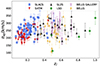 |
Fig. 1. Distribution of the corrected velocity dispersions and redshifts for lensing galaxies in the combined sample from the various surveys. The blue squares represent lenses from SLACS, the green dots represent lenses from LSD, the red down triangles represent lenses from S4TM, the purple crosses represent lenses from BELLS GALLERY, the black triangles represent lenses from SL2S, and the yellow diamonds represent lenses from BELLS. |
3.3. Simulated dataset
We generated synthetic datasets of SN Ia redshifts and galaxy-galaxy strong-lensing observables based on LSST forecast models. This served two main purposes: (a) to assess whether our pipeline can accurately recover the ground truth, and (b) to predict the constraining power of future wide-field surveys such as the LSST. The LSST main survey is expected to detect approximately 400 000 photometrically classified SNe Ia and around 100 000 strong-lensing systems (Collett 2015; Ivezić et al. 2019). For our simulations, we assumed a flat ΛCDM cosmology with ΩM = 0.3 and h = 0.7, which is consistent with the simulated strong-lens population of Collett (2015).
The simulated SNe Ia dataset was divided into two groups: low-redshift (z < 0.16) and high-redshift SNe Ia. For the low-redshift group, we generated 12 000 SNe Ia with spectroscopic redshifts by scaling up from the redshift distribution of current Zwicky Transient Facility (ZTF) observations, which recorded over 3000 SNe Ia in 2.5 years (Dhawan et al. 2022). For the high-redshift sample, we simulated 400 000 SNe Ia with spectroscopic redshifts and adopted the Pantheon+ redshift distribution. In the high-redshift group, redshift bins of 0.05 were used for 0.1 < z ≤ 0.7, and bins of 0.5 were applied for z > 0.7. For both redshift groups, the redshifts were randomly assigned in each bin, and the luminosity distances were computed based on the fiducial cosmology described above. We included a relative uncertainty of 10% on the luminosity distance to reflect the typical observational uncertainties in current SN Ia measurements. Figure 2 shows the resulting redshift distribution of the mock SNe Ia.
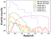 |
Fig. 2. Redshift distributions for the simulated and observed SNe Ia, lenses, and background sources. “obs” represents the observed populations from current observations, and “sim” denotes the mock populations we simulated. |
To model the lens population expected from LSST, we followed the approach of Li et al. (2024), along with the lensing population forecast from Collett (2015). Assuming a spectroscopic confirmation rate for strong lens candidates of 10%, we obtained a sample of 7506 systems with source redshifts below 3.0, which is consistent with spectroscopic galaxy-galaxy lens catalogs. From the SGL population, we took the lens redshifts, source redshifts, and Einstein radii, which we used to calculate the velocity dispersion. During this process, we incorporated probability distributions for the slopes of the mass density (γ and δ) and the anisotropy parameter (β). Specifically, we adopted γ = 2.078 ± 0.16 (Auger et al. 2010) and δ = 2.173 ± 0.085 (Chen et al. 2019), while setting β = 0.22 ± 0.2, as discussed in 4.3.1. In our real-data SGL catalog described in 3.2, we found an average relative error of 11% for  . Hence, we applied this relative uncertainty to the mock velocity dispersion values. No redshift evolution in the lens galaxy properties was assumed. The resulting redshift distributions of the simulated lens and background source populations are also shown in Fig. 2.
4. Method
This section details the method we used to reconstruct the distance and to constrain the density slope of the lensing galaxies, including their evolution with redshift. For reproducibility, the code we used is publicly available on GitHub4.
4.1. Distance reconstruction through ANN
Distance measurements are a critical aspect of the SGL analysis, as they are intricately linked to the observed data and the underlying cosmological model. SGL modeling tools often rely on a fiducial model, such as the vanilla ΛCDM cosmology, to calculate angular diameter distances. SGL systems have proven to be an effective cosmological probe independent of the distance ladder, enabling the determination of key parameters such as the matter energy density Ωm and the cosmic equation of the state parameter w, as highlighted by Chae (2007), Oguri et al. (2008), Biesiada et al. (2010), Cao et al. (2015), Liu et al. (2019). Thus, the ideal scenario would be to measure this quantity independently of any specific cosmological model. This would provide a direct measurement and make it less susceptible to biases inherent in cosmology-dependent methods. We derived the distances directly from the objects at the corresponding redshifts and only assumed a flat and transparent universe.
Artificial neural networks are powerful computational tools inspired by the structure and function of the human brain. They excel at identifying complex patterns within data. An ANN is built from interconnected processing units called neurons, which are arranged in layers. Each neuron applies a nonlinear mathematical function (activation function) to its input, and the outputs are then transmitted to the neurons in the subsequent layers. The training process of an ANN involves adjusting the weights associated with these connections to optimize the performance of the network. This optimization minimizes an error function (loss function), which essentially enables the network to learn from the provided data. The universal approximation theorem by Hornik et al. (1990) states that an ANN with at least one hidden layer that contains a finite number of neurons can approximate any continuous function, given a continuous and nonlinear activation function. This remarkable capability allows ANNs to learn the underlying relations within complex datasets such as cosmological data without any predefined model of the functional form. ANNs have been shown to be effective in reconstructing the relation between redshift and luminosity distance for SN Ia (Gómez-Vargas et al. 2023; Dialektopoulos et al. 2023; Shah et al. 2024; Mitra et al. 2024) as well as for other cosmological probes such as cosmic chronometers (Gómez-Vargas et al. 2023; Mukherjee et al. 2022).
We implemented a three-layer ANN with 20 neurons in each layer. The network took the redshift of the SNIa as input and was trained to predict the corresponding angular diameter distance along with the associated error. During the training, the learning rate was set to 0.001. We used the exponential linear unit (ELU, Clevert et al. 2015) activation function for all except the final output layer, as it helps speed up the learning in deep neural networks. Additionally, ELU improves the classification accuracy compared to commonly used activation functions like the rectified linear unit (ReLU, Agarap 2018) function. The hyperparameters of the model, including its structure, were determined through a random grid search. To initialize the network weights, we employed the Xavier uniform initializer (Glorot & Bengio 2010). The entire network was trained from scratch using the ADAM optimizer with its default exponential decay rates (Kingma & Ba 2015). To prevent overfitting, we implemented the early stopping callback from Keras5 that monitors the validation loss and automatically halts training when the validation loss no longer decreases.
4.2. Constraints on the logarithmic density slope with the single-slope model (γ = δ, β = 0)
We commenced our analysis with the simplest scenario: a single-slope lens model. This model assumes no distinction between the total and luminous mass distribution, which results in a single logarithmic density distribution, that is, γ = δ. To estimate the posterior distribution of the model parameters, we employed Markov chain Monte Carlo (MCMC) techniques using the Python module emcee (Foreman-Mackey et al. 2013). This approach allowed us to perform log-likelihood sampling based on the χ2 function defined in Eq. (8). To mitigate potential biases originating from the specific SGL data used in the MCMC analysis, we performed our investigation using various methods. First, we examined the posteriors obtained from individual lenses (Sect. 4.2.1). Second, we analyzed lenses binned by their scale factor and redshift values with a fixed step size (Sect. 4.2.2). Finally, we considered the posteriors derived from the entire lens sample (Section 4.2.3). This multifaceted analysis strategy helped us to ensure the robustness of our conclusions and mitigated the influence that might arise from the characteristics of individual lenses or specific groups of lenses.
We extracted the values of the logarithmic density distribution from the posterior distribution. The median of the posterior distribution represents the most probable value for γ, while the associated uncertainty was estimated using the median absolute deviation (MAD). The MAD is defined as
 (16)
(16)
After obtaining logarithmic density slopes, γ values from the SGL analysis at different distances, we proceeded to extract their redshift dependence. This was achieved by fitting a linear regression to the relation of γ and z.
4.2.1. Individual constraints
For each SGL system, indexed by i, the theoretical distance ratio was calculated as 𝒟ith(γi; [zL, zS, σobs, θE, θeff]i) from the observables. In this approach, we used the MCMC sampling to minimize the χ2 statistic, defined in Eq. (8), for each lensing system individually. The χ2 for the ith individual lensing system is given by (𝒟iobs−𝒟ith)2/[(Δ𝒟iobs)2+(Δ𝒟ith)2]. From the resulting posterior distribution, we derived the median and the MAD of the density slope parameter γi for each system. In order to investigate the redshift evolution of the density slope, we fit a linear relation ( ) to the obtained γi values across different lens redshifts zl, i.
4.2.2. Fixed-bin approach
In contrast to the individual lens analysis detailed in Sect. 4.2.1, this method focuses on minimizing Eq. (8) for a group of lenses. We achieved this by binning the lenses according to two distinct strategies: the redshift, and the scale factor (a).
The first strategy involves binning lenses based on constant redshift intervals. We adopted a bin size of dz = 0.1 spanning the entire redshift range of our lens sample. This approach allowed us a straightforward grouping of lenses with similar redshifts, potentially revealing trends in the data. However, as redshift and distance are not related in a linear way, we also considered a binning strategy based on the scale factor a = 1/(1 + z). We set a constant step size for this binning, calculated as da = (amax − amin)/8 for each subsample. This ensured that the distribution captured significant data trends, particularly in lower-scale factor bins, which are thought to contain at least 5 data points. The distributions of redshifts and scale factors within the bins for the full sample are shown in Fig. 3. The scale factor bins contain more SGL systems at the high-redshift end.
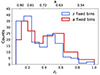 |
Fig. 3. Distribution of the lens redshifts for the full sample. The blue histogram shows bins with fixed redshift intervals, and the red histogram shows bins with fixed scale-factor sizes. |
For a uniform logarithmic density distribution of the total and luminous mass, the theoretical distance ratio for systems in each bin is represented as ![Mathematical equation: $ \mathcal{D}^{th}_i(\gamma^{\mathrm{Sin-bin}}_{\alpha};[z_L,z_S,\sigma_{\mathrm{obs}},\theta_E,\theta_{\mathrm{eff}}]_i) $](/articles/aa/full_html/2025/02/aa51894-24/aa51894-24-eq27.gif) , where the subscript i denotes the ith lensing system within either the α-th fixed-size redshift bin or the α-th fixed-size scale factor bin. Similar to the approach outlined in Sect. 4.2.1, we addressed the redshift evolution of the density slope by conducting a linear fit to the median values and MADs of the posterior distribution of γ from each bin.
, where the subscript i denotes the ith lensing system within either the α-th fixed-size redshift bin or the α-th fixed-size scale factor bin. Similar to the approach outlined in Sect. 4.2.1, we addressed the redshift evolution of the density slope by conducting a linear fit to the median values and MADs of the posterior distribution of γ from each bin.
4.2.3. Full-sample direct fit
This approach deviates from the previously described methods by directly incorporating a redshift evolution of the mass density slope within the MCMC analysis applied to the entire SGL sample. This allowed us to infer the redshift dependence of the mass density slope γ without the need for an intermediate step involving linear fits to the individual γ values obtained from the posterior distribution sampling (Sects. 4.2.1 and 4.2.2).
We still assumed the same mass distribution for the total and luminous components. However, we considered a linear relation between the logarithmic slope of the total mass and the redshift,  , as a universal characteristic of the sample. This affects the theoretical distance ratio as
 ![Mathematical equation: $ \mathcal{D}^{th}_i(\gamma_{0}^{\mathrm{Sin-d}},\gamma_{s}^{\mathrm{Sin-d}};[z_L,z_S,\sigma_{\mathrm{obs}},\theta_E,\theta_{\mathrm{eff}}]_i) $](/articles/aa/full_html/2025/02/aa51894-24/aa51894-24-eq29.gif) for the ith lensing system.
for the ith lensing system.
4.3. Constraints on the logarithmic density slope with an extended spherical power-law model (γ ≠ δ)
In this method, we differentiated between the logarithmic density slopes for total (γ) and luminous (δ) matter in Eq. (3). The anisotropy (β) of the velocity dispersion of the lensing galaxy was also included as a free parameter with a prior. We considered two scenarios for these density slopes: a nonevolving scenario, and a scenario that evolved with redshift.
4.3.1. Anisotropy prior for the velocity dispersions of the lensing galaxy velocity
The dynamical anisotropy of velocity dispersions within lensing galaxies poses a challenge for an accurate modeling. To address this challenge, we explored the impact of different prior distributions for β on our MCMC analysis. We considered three distinct priors:
-
A commonly used truncated Gaussian prior, based on 40 nearby elliptical galaxies from SAURON IFS data (Jorgensen et al. 1995; Bolton et al. 2006), uses β = 𝒩(0.18; 0.13) and is truncated within the range [β − 2σβ, β + 2σβ].
-
We introduce a new prior using the dynamics and stellar population analysis from the MaNGA Survey (SDSS Data Release 17, Zhu et al. 2023b, 2024). The MaNGA Survey uses integral field unit (IFU) data to provide spatially resolved dynamical information for nearly 104 local Universe galaxies, which is analyzed via the axisymmetric Jeans anisotropic modeling (JAM) method. To ensure compatibility with our spherical power-law model, we refined the velocity anisotropy constraints for early-type galaxies using the JAMsph model assuming the general NFW dark matter distribution outlined by Zhu et al. (2023b). The galaxy morphology was sourced from the deep-learning-based catalog by Domínguez Sánchez et al. (2022). To focus on reliable data, we selected only early-type galaxies with a visual quality rating greater than zero from Zhu et al. (2023b), which resulted in a sample of 2597 galaxies. The distribution of their velocity anisotropy values is shown in Fig. 4. From this dataset, we identified a peak value (mode) of βp at 0.102. We established a triangular prior distribution centered at the mode, with bounds at ( − 0.5, 0.656). This encompassed most of the galaxies in the sample.
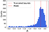
Fig. 4. Distribution of the velocity anisotropy constraints for early-type galaxies from stellar dynamic modeling for the MaNGA survey in the final SDSS DR17 (Zhu et al. 2023b).
-
Based on the same MaNGA sample as described above, Guerrini & Mörtsell (2024) implemented an additional selection criterion. They focused on galaxies for which the absolute difference between the velocity anisotropy values obtained from the NFW model (NFW) and the generalized NFW model (gNFW) was smaller than 0.05 (|βNFW − βgNFW|< 0.05). We applied this criterion to the original MaNGA sample (Zhu et al. 2023b) and obtained a refined selection of 1136 galaxies. The fit of a truncated logistic Gaussian distribution yielded a best-fit prior of β = 𝒩(0.22; 0.2) truncated at [μ − 3σ, μ + 3σ].
4.3.2. Nonevolving lens model
The nonevolving scenario assumes that our SGL systems can be effectively described by the extended power-law model with some constant values of γ and δ that are representative of the whole sample. The theoretical distance ratio for each lensing system is represented as 𝒟ith(γEPL − n, δEPL − n, β; [zL, zS, σobs, θE, θeff]i), where the anisotropy parameter β is not a free parameter, but is represented by a certain prior, as discussed in Sect. 4.3.1.
4.3.3. Evolving lens model
Similar to the single-density slope model, we implemented different approaches to explore the features of a potential redshift evolution. We only applied the fixed-bin and the direct approach to do this because the three-parameter constraint performs poorly on individual SGL system. For the fixed-bin approach, we independently determined the density slopes in each bin without accounting for redshift evolution, and we subsequently fit these constraints linearly in the bins to identify any evolutionary trends. The direct approach adopts two semi-analytical models for the redshift evolution. The first model is linear evolutions for γ and δ with respect to the lens redshift zL, represented as
 (17)
(17)
where the superscript EPL−lin denotes the linear evolution parameters under the extended spherical power-law model.
In order to determine the evolution with respect to the scale factor, we considered the second evolving model as
 (18)
(18)
where the superscript EPL−ATE denotes that the evolution model comes from the Taylor expansion in terms of the scale factor. In order to compare the performance of different β priors and evolving scenarios, we employed corrected Akaike information criterion (cAIC) and Bayesian information criterion (BIC) evaluations. They are defined as
 (19)
(19)
where k is the number of parameters, and N is the number of data points. The BIC assesses the model quality by approximating −2ln(marginal likelihood) with fitting the maximum likelihood estimation. Additionally, it adds a penalty to the complexity based on the number of parameters. The cAIC is also commonly used for the model selection, and it adjust for small-sample size data based on the standard AIC. The cAIC only differs from the BIC in its penalty term.
5. Results
5.1. Distance reconstruction
We employed the model-independent ANN method, which performed without assuming any specific cosmology parameters, just a flat transparent ΛCDM structure, to reconstruct the angular diameter distance at various redshifts. The resulting distance-redshift relations are visualized in Fig. 5. Despite the limited number of high-redshift data points, the reconstructed distance-redshift relation accurately captures the expected feature of the angular diameter distance, notably showing an inflection point around redshift 1.5. These reconstructed distances served as the foundation for calculating the observed distance ratio 𝒟obs (see Eq. (7)) for each lensing system within our analysis.
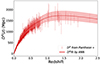 |
Fig. 5. Reconstruction of the angular diameter distance under nonparametric methods. The red dots indicate the angular diameter distance calculated from the measurements of SNIa. The red line represents the best-fit distance reconstruction by ANN+SNIa. The shadowed region shows the 1σ uncertainties for the corresponding distance reconstruction. |
5.2. Constraints from the single-density slope model
In this section, we present the constraints on the redshift evolution of the density slope γ of single uniform density distributions using the individual approach, the binning approach, and the direct method. The best-fit values for γ0Sin and the slopes γsSin are listed in the Table 1. The results from the individual method suggest that γ decreases with increasing redshift, as shown by ∂γSin − I/∂zL = −0.141 ± 0.033, and as displayed in Figure 6.
Summary of the constraints on the intercept (γ0) and slope (γs = ∂γ/∂zL) of the linear redshift evolution for different approaches.
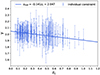 |
Fig. 6. Linear fit for the individual constraints on the logarithmic slope γ. |
The best-fit linear redshift evolution of γ as analyzed in fixed-size bins is depicted in Fig. 7. Within the fixed-size redshift bins, the combined sample indicates a redshift evolution for the density slope γSin − zbin = 2.063(±0.015)−zL × 0.316(±0.053). For the fixed-size scale factor bins, the best-fit linear redshift evolution of γ presents γSin − abin = 2.070(±0.013)−zL × 0.311(±0.036). The results of different binning approaches agree well with each other. Fig. 7 shows that because there are only a few observations with a redshift close to one, the uncertainty increases in these bins.
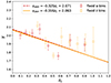 |
Fig. 7. Linear fit for γ constrained in fixed-redshift bins. The empty red circles represent the results in fixed-scale factor bins, and the empty orange squares denote the results in fixed-redshift bins. |
In the direct constraining approach that assumes a global redshift evolution, the results yield γSin − d = 2.069(±0.028)−zL × 0.294(±0.073). Despite the considerable uncertainties for each SGL system in the individual approach, it shows a lower uncertainty than other approaches. Compared to the individual approach, the binning method and the direct approach suggest a steeper redshift evolution for lensing galaxies.
5.3. Constraints with γ ≠ δ model
5.3.1. Nonevolving γ and δ
Assuming a static mass model, we constrained the density slopes of the total mass and luminous matter using the different anisotropy priors described in Sect. 4.3.1. For the median values and MAD of the posterior distributions, the triangular prior yields a total mass density slope of γEPL − n = 1.987 ± 0.031 and a luminous density slope of δEPL − n = 2.16 ± 0.16. A Gaussian prior, suggested by Guerrini & Mörtsell (2024), indicates γEPL − n = 1.993 ± 0.032 and δEPL − n = 2.29 ± 0.12. Another Gaussian prior from Bolton et al. (2006) results in γEPL − n = 1.998 ± 0.032 and δEPL − n = 2.298 ± 0.092. As depicted in Fig 8, a strong degeneracy exists between the velocity anisotropy parameter β and the luminous matter density slope δ, highlighting the necessity of selecting a reasonable β prior. A narrower range for β provides more stringent constraints on δ, but does not significantly affect the constraining power on γ. When the redshift evolution was not considered, the spherical model displayed a bimodal distribution in the γ constraints, indicating possible variations in the total mass density slope of lensing galaxies that may be related to other quantities, such as redshift or velocity dispersions.
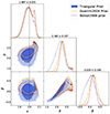 |
Fig. 8. Constraints on the logarithmic density slope of the total mass and the luminous mass in the nonevolution picture. The blue contours indicate the posterior distribution adopting the triangular prior of β defined in Sect. 4.3.1. The yellow and red contours indicate the posterior distribution adopting the Gaussian priors of β based on Guerrini & Mörtsell (2024) and Bolton et al. (2006), respectively. The dashed black line corresponds to a singular isothermal sphere. |
5.3.2. Evolving γ and δ
With the full sample, we first used the binning approach to constrain the density slope in the redshift and scale factor bins and then fit the linear redshift evolution. As shown in Table A.1, the total mass density slopes from different β priors show a strong negative redshift evolution, and they do not deviate significantly. Conversely, the constraint on the δ evolution varies with the change in the β priors.
Next, we directly applied linear redshift evolution models to the mass density slopes. In order to ensure the precision of our constraints, we selected lensing systems where the relative uncertainty in the normalized velocity dispersion ( ) was smaller than 20%. This criterion restricted our sample to 132 lensing systems with well-constrained velocity dispersions, and it can therefore alleviate the potential systemic errors in determining the mass density slope. The constraints from the triangular prior for the linearly evolving spherical model show a median total mass density slope (γ0) of 2.065 ± 0.046 and a redshift evolution gradient (γs) of −0.20 ± 0.12. The luminous mass density slope intercept (δ0) is 2.14 ± 0.16, with a gradient (δs) of −0.09 ± 0.19. The results in Fig. 9 indicate a slight negative redshift evolution for the total and luminous mass densities, without ruling out a nonevolving scenario for luminous matter within 1σ uncertainty. The result also confirms that the luminous mass density slope is steeper than that of the total mass. Strong degeneracies are observed between δ0 and β. The comparison of the results from different β priors in Table A.2 shows that the wider range of the triangular prior matches the constraining strength of the narrower Gaussian priors for the γ evolution constraints.
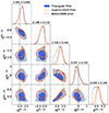 |
Fig. 9. Posterior distributions of the spherical power-law density model parameters with linear redshift evolution. The blue contours indicate the posterior distribution adopting the triangular prior of β defined in Sect. 4.3.1. The yellow and red contours indicate the posterior distribution adopting the Gaussian priors of β based on Guerrini & Mörtsell (2024) and Bolton et al. (2006), respectively. The dashed black line corresponds to the singular isothermal sphere. |
We finally applied the ATE evolution model to the mass density slopes with three β priors. In Figure 10, the triangular prior yields a redshift evolution of the total mass density slope of γEPL − ATE = 2.079(±0.056)−0.35(±0.23)×z/(1 + z), and the redshift evolution of the luminous mass density slope is δEPL − ATE = 2.17(±0.17)−0.25(±0.40)×z/(1 + z). In contrast to the linear evolution, the ATE redshift evolution model indicates a steeper density slope of the total mass at lower redshifts and aligns more closely with the isothermal behavior at higher redshifts. The triangular prior is again preferred by cAIC and BIC under the ATE evolution model, but it is surpassed by the linear evolution model with the triangular prior. In the different parametric models, all constraints show a negative redshift evolution in the total mass density slope of the lensing galaxies. Moreover, the 1σ uncertainty region of the best-fit models from the linear and ATE parameterization encompasses the isothermal scenario.
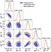 |
Fig. 10. Posterior distributions of the spherical power-law density model parameters under ATE evolution. The blue contours indicate the posterior distribution adopting the triangular prior of β (see Sect. 4.3.1). The yellow and red dashed contours represent the posterior distribution derived from Gaussian priors on β following Guerrini & Mörtsell (2024) and Bolton et al. (2006), respectively. The dashed black line corresponds to the case of the singular isothermal sphere. |
5.4. Constraints based on the simulation data
The relation between redshift and distance as reconstructed from mock SNe Ia data is displayed in Fig. 11. The ANN effectively reproduces the fiducial redshift-distance function anticipated in the flat ΛCDM model. This demonstrates the precision of our method. For the mock SGL data, we employed the individual approach with a single-density slope model, the binning approach, and the direct method using an EPL model to assess the redshift evolution. The individual approach provided the constraint γsim = 1.985(±0.003)+zL × 0.004(±0.006), indicating a nearly constant density slope. However, the mean total density slope deviates from the fiducial value because the EPL model we used to generate the data and the SIS model we assumed in the individual analysis do not match. The results from the binning approach are presented in Figure 12. The redshift and scale-factor binning successfully recover the fiducial values within the 68% confidence interval, in particular for the total mass density slope at z ≤ 1. For z > 1, some deviations in γ and δ are observed, which are further discussed in Sect. 6.2. In comparison, the anisotropy parameter β demonstrates greater robustness than the parameters of the mass density slope.
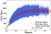 |
Fig. 11. Reconstruction of the angular diameter distance using mock SNe Ia data. The green and blue dots indicate the angular diameter distance calculated from low-z and high-z SNe Ia, respectively. The solid orange line indicates the redshift-distance relation based on a flat ΛCDM cosmology with ΩM = 0.3 and h = 0.7. The dashed red line represents the best-fit distance reconstruction obtained by ANN+SNIa. The shaded region shows the corresponding 1σ uncertainties. |
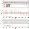 |
Fig. 12. Constraints on the density slope parameters for redshift bins (empty orange squares) and scale factor bins (empty red circles). The gray shaded regions represent the 1σ intervals for the fiducial density slope parameters for the simulation. |
The direct constraints on the density slope parameters from the mock data are shown in Figure 13. These parameters are also recovered within a 68% confidence level. Compared to the parameters related to the luminosity matter density and anisotropy, the total mass density parameters (γ0 and γs) are constrained with higher precision. The simulation results reveal significant degeneracies, similar to those observed in real data, particularly between the parameters δ0 and β, and also between γs and δs. These correlations mainly result from the physical interaction between the luminous tracer and the total mass distribution. High-precision dynamical measurements, such as those provided by integral field units (IFUs), have the potential to break the degeneracy between δ0 and β, thereby offering tighter constraints on the evolution parameter δs for luminous tracers. Unlike the individual and binning methods, the direct constraining approach shows reduced sensitivity to outliers in the data, making it a robust alternative for a parameter estimation in the presence of anomalous data points.
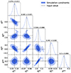 |
Fig. 13. Posterior distributions of the spherical power-law density model parameters for 7506 SGL mock data. The dashed black lines indicate the fiducial values we used to generate the mock data. |
6. Discussions
In this section, we explore several aspects of our method and findings. In Sect. 6.1, we discuss the combination of nonparametric methods and model-independent observations for the distance reconstruction. Sect. 6.2 addresses potential biases in our analysis, and Sect. 6.3 considers additional dependences of the total mass density slope on the lens galaxy properties. Finally, in Sect. 6.4, we compare the differences of the derived constraints on the total mass density slope in multiple approaches and under varying priors.
6.1. Reconstructing the distance with model-independent observations
The SGL systems are increasingly recognized as valuable cosmological probes. While their capability for constraining the Hubble constant (H0) through time-delay cosmography is well established, SGL systems can also be harnessed to investigate additional cosmological parameters, including the matter density (Ωm), cosmic curvature (Ωk), and the dark energy equation of state (w). Their sensitivity to these parameters has been well documented (Suyu et al. 2014; Cao et al. 2015; Arendse et al. 2019; Liu et al. 2019; Liao et al. 2019, 2020; Wong et al. 2020; Qi et al. 2021; Li et al. 2024), but it is often not adequately taken into account in current approaches to lens modeling. Conventional modeling typically relies on a fiducial cosmological model to calculate distances at specific redshifts, which might introduce systematic biases. To mitigate these biases and avoid circular reasoning, we constrained the lens model and its redshift evolution solely using observational distance indicators and did not assume any specific cosmological parameters in the flat ΛCDM framework. This method only provides discrete measurements at certain redshifts, however, and requires a suitable reconstruction of the redshift–distance relation to properly match each SGL system.
Our analysis used ANNs, a nonparametric method, to reconstruct the angular diameter distance at various redshifts. ANN is proven to be effective in smoothing and accurately reconstructing the redshift-distance relation, as demonstrated in Fig. 11 by our simulations that were trained with extensive SNe Ia data. The method is also capable of extrapolating beyond the limits of the existing data. However, the precision of the reconstruction is limited by the sample size; a smaller dataset can reduce the accuracy of the results.
6.2. Potential sources of bias
When interpreting our findings, it is important to consider potential biases that might affect the accuracy and reliability of results. A significant source of bias may stem from deviations in the ANN reconstruction for DA, especially for data involving high redshifts. As illustrated in Figure 12, the total mass density slope γ begins to deviate at z ≳ 1. Two key factors contribute to this deviation. First, our sample lacks sufficient lensing galaxy data at z > 1, which is depicted in Fig. 14. The distance ratio that we used to constrain the density slope parameters, relies on the reconstructed distances from the lens and the source. Without direct observational constraints above z = 2.2, these source distances must be extrapolated from the ANN-based reconstruction. Second, any deviation from the fiducial cosmology in this extrapolation, especially at z > 2.2, can further skew the inferred density slope parameters. These considerations underscore the importance of careful treatment in future analyses. Insufficient sample sizes and uncertainties in high-redshift extrapolations may similarly affect the density slope measurements in real observational datasets, highlighting the need for more comprehensive data coverage at the high-redshift end.
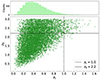 |
Fig. 14. Redshift distribution of the simulated SGL. The top histogram shows the redshift distribution of mock lensing galaxies. The dashed black line indicates the lens redshift zL = 1.0. The solid black line indicates the source redshift zS = 2.2, which is the upper limit for the SNe Ia simulation. |
Another potential source of bias might be the correction for the velocity dispersion aperture, which may not be appropriate for all measurements. The velocity dispersions (σap) in our sample are measured within different fiber apertures, while the lensing galaxies have different angular sizes that span a wide dynamic range. To normalize the measured velocity dispersions to a physically meaningful radius, which is half of the effective radius (θeff) in this work, we applied an aperture correction. We used the power-law function proposed by Jorgensen et al. (1995) to quantify the power-law slopes of the normalized σap profiles (see Eq. (13)). The parameters of the correction function were determined by Cappellari et al. (2006) based on the SAURON IFS data from 40 ETGs. However, Zhu et al. (2023a) demonstrated that these parameters may not be applicable to galaxies with intermediate Sérsic indices, and the power-law index of the correction function strongly depends on the r-band absolute magnitude Mr, g − i color, and Sérsic index nser. We lacked the complete information needed to customize the aperture correction for each lensing system, and the changes in the aperture correction can lead to additional bias. A detailed study of the application of customized aperture corrections for the lensing galaxies is in preparation.
Additionally, the simplicity of the lens model adopted in our study may introduce additional biases in the constraints. We assumed that the total mass and the luminous tracer in all strongly gravitationally lensing (SGL) systems follow a spherical power-law profile. Moreover, while anisotropy can vary in different galaxies, our analysis treated it as a universal value for all systems, and we only applied a broad prior. These assumptions are strong and may not hold in all cases. Deviations from the power-law model, particularly in the stellar mass distribution, have been reported in studies such as Etherington et al. (2023), Tan et al. (2024). Although the power-law model is proven to be valid at the population level, it may deviate from the true value when extreme systems are present in a relatively small subsample.
6.3. Other possible dependences of the evolution on the density slope constraints
In analyzing a nonevolving EPL model, we detected bimodal characteristics in the posterior distribution of the total mass density slope (γ), with a primary peak at γ = 1.987 and a secondary slightly steeper peak. This suggests a potential internal divergence or temporal variation in γ. Our study primarily investigated the redshift evolution of γ, which agrees with the findings from other studies, but also acknowledged the significance of the internal divergence. Etherington et al. (2023) explored additional variables such as a normalized Einstein radius θE/θeff and velocity dispersions, which are motivated by lensing and dynamics (Sonnenfeld et al. 2012; Auger et al. 2010; Li et al. 2018).
Cao et al. (2016) documented a divergence in γ with respect to the velocity dispersion by categorizing galaxies into low-, intermediate-, and high-mass based on their velocity dispersion measurements. They noted a decrease in γ with increasing velocity dispersion in a single-density slope model, but no such trend when γ ≠ δ. Conversely, Etherington et al. (2023) observed an increase in γ at a higher velocity dispersion. We adopted a similar approach as Etherington et al. (2023) and examined the linear relation between the velocity dispersion and γ for the total and luminous mass. With the truncated triangular β prior mentioned in Sect. 4.3.1, our fitting yielded the relation γ(σv) = 1.22(±0.13)+0.59(±0.13)×log10(σv), which supports the results from Etherington et al. (2023). For the dependence on the radius, Li et al. (2018) found that the total mass density slope has an increasing trend with normalized Einstein radii, while Etherington et al. (2023) reported a slightly decreasing trend. We also assessed the impact of the normalized Einstein radius on γ and found a linear relation as  , which is consist with the work using the BELLS, GALLERY, and SL2S samples in Li et al. (2018).
In order to determine whether our results can be used as an effective model of population of lenses, we inferred γ by using redshifts of lensing galaxies and our best-fitting evolution models under triangular β priors. Then we compared the resulting distribution of model-predicted γ exponents with the results of a detailed modeling (Etherington et al. 2023) based on observations from 123 lensing galaxies from the SLACS, BELLS, GALLARY, SL2S, and LSD surveys. For comparison, we also presented the predictions based on γ(σv) and γ(θE,nor) regression models. As shown in Fig. 15, the γ populations derived from linear evolution models based on the velocity dispersion and normalized Einstein radii tend to concentrate around lower γ values, while our sample of generated γ indices closely aligns within the 1 σ uncertainty of the lensing+dynamics modeling results. This consistency supports the hypothesis that the redshift-evolving extended power-law model is valid for describing lensing galaxies at the population level.
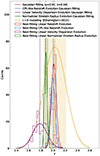 |
Fig. 15. Regenerated γ distributions from various evolutionary models. The red, blue, purple, and green steps represent the distributions from the best-fit linear redshift, ATE, linear velocity dispersion, and linear normalized Einstein radius evolution models, respectively. The solid yellow line indicates the γ distribution from lensing and dynamics modeling (Etherington et al. 2023), and the shaded area represents the 1σ uncertainty. The dashed lines in all colors mark the mean values from Gaussian fits of each distribution. |
6.4. Comparing constraints Across Different Approaches and Priors
Across various methods, the redshift evolution of the total mass density slope (γ) of the lensing galaxy consistently indicates either a slightly negative trend or no significant change with increasing redshift. In the case of a single-density slope, the individual constraints have the smallest uncertainties, but with flatter evolution slopes than in other two methods.
In the case of γ ≠ δ, we adopted three different priors for the anisotropy (β) of the velocity dispersion for lensing galaxies. Based on 2597 early-type galaxies analyzed using the axisymmetric JAM method assuming a general NFW dark matter distribution, the triangular prior described the anisotropy distribution over a broad range. The Gaussian prior, based on the same sample but with an additional selection, provided a more consistent and concentrated anisotropy distribution. The differences among the priors do not significantly affect the constraints on the total mass density, but do impact the luminous matter density slope and its redshift evolution. To describe the redshift evolution of the total mass density slope, we considered two semi-analytical evolution models for the direct approach. The linear model is straightforward and widely used to search for evolving trends, while the ATE evolving scenario has a physical basis and is applicable for cases with higher redshifts.
Compared to other studies (Sonnenfeld et al. 2013b; Remus et al. 2017; Chen et al. 2019; Etherington et al. 2023; Tan & Shajib 2024) of the same topic in Fig. 16, our results support a slightly negative or no-evolution scenario for the total mass density slope as the redshift increases. The evolution trend is consistent with work based on lensing and dynamic measurements (Sonnenfeld et al. 2013b; Cao et al. 2016; Holanda et al. 2017; Chen et al. 2019). However, the redshift evolution constraints based on lensing-only data prefer a positive evolution picture (Etherington et al. 2023; Tan & Shajib 2024). This is supported by Magneticum Pathfinder1 simulations, which suggest that gas-poor mergers dominate the evolution phase at lower redshifts (Remus et al. 2017). Etherington et al. (2023) pointed out that these differences may arise because the physical meaning of the density slope differs in lensing+dynamics and lensing-only methods. They argued that the lensing+dynamics method tends to measure the mass-weighted density slope within the effective radius, while the lensing-only method measures the local density slope around the Einstein radius.
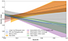 |
Fig. 16. Total density slope of early-type galaxies as a function of redshift. The dotted blue line represents the best fit using the linear evolution model with a triangular β prior, and the solid blue line represents the best fit using the ATE evolution model with the triangular prior described in Sect. 4.3.1. The dashed dark green line indicates the average total density slope from the Magneticum simulations (Remus et al. 2017). The light orange band shows the 1σ uncertainty region of constraints on elliptical galaxy mass profile evolution from Tan & Shajib (2024). The diagonal striped purple band represents the total density constraints based on lensing and dynamic information from the SL2S, SLACS, and LSD surveys. The circled red band shows the total density slope evolution constraints obtained by fitting the source light in every pixel of Hubble Space Telescope images from Etherington et al. (2023). The backward striped gray band indicates the lensing+dynamics constraints for overlapping systems with pixelized light-fitting constraints from Etherington et al. (2023). The dotted green band represents the single-density slope evolution constraints with the same sample as used in this paper from Chen et al. (2019). |
In the redshift range z > 0.4, the total density slope deviates between results from lensing+dynamics and lensing-only methods in Fig. 16. The lensing-only results prefer steeper slopes, while the lensing+dynamics results favor slopes that are flatter than the isothermal case. This difference in constraints on the redshift evolution suggests that the SGL sample is not large enough and is still easily affected by uncertain local data points. Moreover, the lensing systems we used to constrain the redshift evolution differ, which may affect the results through the selection effects. In order to avoid a selection effect, Etherington et al. (2023) compared an overlapping sample with total mass density slope constraints from the lensing+dynamics and lensing-only methods. They found that the results from lensing+dynamics prefer an almost no-evolution scenario, while the lensing-only results support a positive redshift evolution as the redshift increases.
7. Summary
This study presents a novel approach that is independent of the dark energy model for reconstructing the distance ratios of SGL systems to constrain the mass-density slope and its redshift evolution. To the best of our knowledge, this is the first application of such a method in this field. To achieve this, we employed a nonparametric ANN method. Using observations of SNIa, we reconstructed distance ratios and compared them to theoretical predictions. This analysis allowed us to estimate the redshift evolution of the EPL parameters for a sample of 161 lensing galaxies from the LSD, SL2S, SLACS, S4TM, BELLS, and BELLS GALLERY surveys. Mock data, generated using future survey forecasts, were employed to evaluate whether our method was able to accurately recover the input fiducial value and to forecast its constraining power. Based on our results, we draw the following conclusions:
-
The internal divergence in a nonevolving analysis, as observed in Sect. 5.3.1, highlights the need to account for redshift evolution in density slopes when analyzing lensing galaxies. Employing a triangular prior on the velocity dispersion anisotropy β, based on recent MaNGA DynPop dynamical modeling (Zhu et al. 2024), and a linear redshift evolution model, our best-fit model indicates a redshift evolution as γ = 2.065(±0.046)−0.20(±0.12)×z for the total mass, and δ = 2.14(±0.16)−0.09(±0.19)×z for the luminous matter.
-
Although observational evidence indicates that the extended power-law (EPL) may not suit individual lens modeling (Treu et al. 2006; Humphrey & Buote 2010; Etherington et al. 2023; Tan et al. 2024), we found that it remains valid at the population level. This finding supports the use of the so-called bulge-halo conspiracy to reduce the degrees of freedom in statistically constraining cosmological parameters. As discussed in Sect. 6.3, we observe that the EPL parameters evolve more strongly with redshift than other physical quantities.
-
The deviation across different studies may imply that the current sample of lensing galaxies remains too small to produce consistent and robust results regarding the evolution of lenses. This highlights the urgent need for large surveys to uncover new SGL systems and build a more complete dataset. Wide-area high-sensitivity optical surveys such as the LSST from the Vera C. Rubin Observatory, along with complementary spectroscopic follow-ups using instruments such as 4MOST (Depagne 2015) and advanced techniques like IFU (Zhu et al. 2024), will provide us with a larger and more comprehensive sample (Collett 2015). The simulation results indicate that increasing the SGL sample size by a factor of 50 could enhance the precision of the total mass density slope evolution to Δ(∂γ/∂z)∼0.021. This improvement would also aid in resolving discrepancies between lensing+dynamics and lensing-only constraints on the redshift evolution of the total mass distribution in early-type galaxies (Etherington et al. 2023). Furthermore, it would provide deeper insights into the differences between gravitational and dynamical mass measurements of lensing galaxies.
By “model-independent” we refer to the approach of not assuming any fixed background cosmology such as an ΛCDM model with definite (fiducial) values of the Hubble constant, matter density parameter, and dark energy density parameters. A more fitting name would be an approach that is agnostic to the dark energy model. We point out that the term “model-independent” approach is still used, but it is almost impossible to avoid prior cosmological assumptions such as the (flat) FLRW model or Etherington principle (i.e., the distance duality relation), as we spelled out explicitly in the text.
In order to avoid confusion with the velocity dispersion we denote the uncertainty by Δ instead of commonly used σ.
Acknowledgments
This research was supported by the Polish National Science Center grant 2023/50/A/ST9/00579 and the program of China Scholarships Council. Thanks for the referee for their constructive suggestions to help with this manuscript.
References
- Abbott, B. P., Abbott, R., Abbott, T. D., et al. 2017, Nature, 551, 85 [Google Scholar]
- Acevedo Barroso, J. A., O’Riordan, C. M., Clément, B., et al. 2024, A&A, submitted [arXiv:2408.06217] [Google Scholar]
- Agarap, A. F. 2018, arXiv e-prints [arXiv:1803.08375] [Google Scholar]
- Arendse, N., Agnello, A., & Wojtak, R. J. 2019, A&A, 632, A91 [NASA ADS] [CrossRef] [EDP Sciences] [Google Scholar]
- Asgari, M., Lin, C.-A., Joachimi, B., et al. 2021, A&A, 645, A104 [NASA ADS] [CrossRef] [EDP Sciences] [Google Scholar]
- Auger, M. W., Treu, T., Bolton, A. S., et al. 2009, ApJ, 705, 1099 [Google Scholar]
- Auger, M. W., Treu, T., Bolton, A. S., et al. 2010, ApJ, 724, 511 [NASA ADS] [CrossRef] [Google Scholar]
- Biesiada, M., Piórkowska, A., & Malec, B. 2010, MNRAS, 406, 1055 [NASA ADS] [Google Scholar]
- Bolton, A. S., Rappaport, S., & Burles, S. 2006, Phys. Rev. D, 74, 061501 [CrossRef] [Google Scholar]
- Bolton, A. S., Burles, S., Koopmans, L. V. E., et al. 2008, ApJ, 682, 964 [Google Scholar]
- Bora, K., Holanda, R. F. L., & Desai, S. 2021, Eur. Phys. J. C, 81, 596 [NASA ADS] [CrossRef] [Google Scholar]
- Brownstein, J. R., Bolton, A. S., Schlegel, D. J., et al. 2012, ApJ, 744, 41 [NASA ADS] [CrossRef] [Google Scholar]
- Cao, S., Zhu, Z.-H., & Zhao, R. 2011, Phys. Rev. D, 84, 023005 [NASA ADS] [CrossRef] [Google Scholar]
- Cao, S., Covone, G., & Zhu, Z. 2012a, ApJ, 755, 31 [NASA ADS] [CrossRef] [Google Scholar]
- Cao, S., Pan, Y., Biesiada, M., Godlowski, W., & Zhu, Z. 2012b, JCAP, 2012, 016 [CrossRef] [Google Scholar]
- Cao, S., Biesiada, M., Gavazzi, R., Piórkowska, A., & Zhu, Z.-H. 2015, ApJ, 806, 185 [NASA ADS] [CrossRef] [Google Scholar]
- Cao, S., Biesiada, M., Yao, M., & Zhu, Z.-H. 2016, MNRAS, 461, 2192 [CrossRef] [Google Scholar]
- Cao, S., Qi, J., Cao, Z., et al. 2019, Sci. Rep., 9, 11608 [NASA ADS] [CrossRef] [Google Scholar]
- Cappellari, M., Bacon, R., Bureau, M., et al. 2006, MNRAS, 366, 1126 [Google Scholar]
- Chae, K. 2007, ApJ, 658, L71 [Google Scholar]
- Chen, Y., Li, R., Shu, Y., & Cao, X. 2019, MNRAS, 488, 3745 [NASA ADS] [CrossRef] [Google Scholar]
- Cheng, W., He, Y., Diao, J.-W., et al. 2021, J. High Energy Phys., 2021, 124 [CrossRef] [Google Scholar]
- Clevert, D. A., Unterthiner, T., & Hochreiter, S. 2015, arXiv e-prints [arXiv:1511.07289] [Google Scholar]
- Cole, S., Percival, W. J., Peacock, J. A., et al. 2005, MNRAS, 362, 505 [Google Scholar]
- Colgate, S. A., & McKee, C. 1969, ApJ, 157, 623 [NASA ADS] [CrossRef] [Google Scholar]
- Collett, T. E. 2015, ApJ, 811, 20 [NASA ADS] [CrossRef] [Google Scholar]
- Depagne, É. 2015, in Asteroseismology of Stellar Populations in the Milky Way, eds. A. Miglio, P. Eggenberger, L. Girardi, & J. Montalbán, Astrophys. Space Sci. Proc., 39, 147 [NASA ADS] [Google Scholar]
- DESI Collaboration (Adame, A. G., et al.) 2024, arXiv e-prints [arXiv:2404.03002] [Google Scholar]
- Dhawan, S., Goobar, A., Smith, M., et al. 2022, MNRAS, 510, 2228 [NASA ADS] [CrossRef] [Google Scholar]
- Dialektopoulos, K. F., Mukherjee, P., Said, J. L., & Mifsud, J. 2023, Eur. Phys. J. C, 83, 956 [NASA ADS] [CrossRef] [Google Scholar]
- Di Valentino, E., Mena, O., Pan, S., et al. 2021, Class. Quantum Gravity, 38, 153001 [NASA ADS] [CrossRef] [Google Scholar]
- Domínguez Sánchez, H., Margalef, B., Bernardi, M., & Huertas-Company, M. 2022, MNRAS, 509, 4024 [Google Scholar]
- Eisenstein, D. J., Zehavi, I., Hogg, D. W., et al. 2005, ApJ, 633, 560 [Google Scholar]
- Etherington, A., Nightingale, J. W., Massey, R., et al. 2023, MNRAS, 521, 6005 [CrossRef] [Google Scholar]
- Foreman-Mackey, D., Hogg, D. W., Lang, D., & Goodman, J. 2013, PASP, 125, 306 [Google Scholar]
- Gayathri, V., Healy, J., Lange, J., et al. 2020, arXiv e-prints [arXiv:2009.14247] [Google Scholar]
- Geng, S., Cao, S., Liu, Y., et al. 2021, MNRAS, 503, 1319 [NASA ADS] [CrossRef] [Google Scholar]
- Glorot, X., & Bengio, Y. 2010, in Proceedings of the Thirteenth International Conference on Artificial Intelligence and Statistics, AISTATS 2010, Chia Laguna Resort, Sardinia, Italy, May 13–15, 2010, eds. Y. W. Teh, & D. M. Titterington (JMLR.org), JMLR Proceedings, 9, 249 [Google Scholar]
- Gómez-Vargas, I., Medel-Esquivel, R., García-Salcedo, R., & Vázquez, J. A. 2023, Eur. Phys. J. C, 83, 304 [CrossRef] [Google Scholar]
- Guerrini, S., & Mörtsell, E. 2024, Phys. Rev. D, 109, 023533 [CrossRef] [Google Scholar]
- Harnois-Déraps, J., Heydenreich, S., Giblin, B., et al. 2024, MNRAS, 534, 3305 [CrossRef] [Google Scholar]
- Holanda, R. F. L., Pereira, S. H., & Jain, D. 2017, MNRAS, 471, 3079 [CrossRef] [Google Scholar]
- Hornik, K., Stinchcombe, M., & White, H. 1990, Neural Netw., 3, 551 [CrossRef] [Google Scholar]
- Hoyle, F., & Fowler, W. A. 1960, ApJ, 132, 565 [NASA ADS] [CrossRef] [Google Scholar]
- Humphrey, P. J., & Buote, D. A. 2010, MNRAS, 403, 2143 [Google Scholar]
- Ivezić, Ž., Kahn, S. M., Tyson, J. A., et al. 2019, ApJ, 873, 111 [Google Scholar]
- Jiang, G., & Kochanek, C. S. 2007, ApJ, 671, 1568 [NASA ADS] [CrossRef] [Google Scholar]
- Jorgensen, I., Franx, M., & Kjaergaard, P. 1995, MNRAS, 276, 1341 [NASA ADS] [Google Scholar]
- Kingma, D. P., & Ba, J. 2015, in 3rd International Conference on Learning Representations, ICLR 2015, San Diego, CA, USA, May 7–9, 2015, Conference Track Proceedings, eds. Y. Bengio, & Y. LeCun [Google Scholar]
- Koopmans, L. V. E. 2006, in EAS Publications Series, eds. G. A. Mamon, F. Combes, C. Deffayet, & B. Fort, 20, 161 [NASA ADS] [CrossRef] [EDP Sciences] [Google Scholar]
- Koopmans, L. V. E., & Treu, T. 2002, ApJ, 568, L5 [NASA ADS] [CrossRef] [Google Scholar]
- Koopmans, L. V. E., & Treu, T. 2003, ApJ, 583, 606 [NASA ADS] [CrossRef] [Google Scholar]
- Kormann, R., Schneider, P., & Bartelmann, M. 1994, A&A, 284, 285 [NASA ADS] [Google Scholar]
- Li, R., Shu, Y., & Wang, J. 2018, MNRAS, 480, 431 [NASA ADS] [CrossRef] [Google Scholar]
- Li, T., Collett, T. E., Krawczyk, C. M., & Enzi, W. 2024, MNRAS, 527, 5311 [Google Scholar]
- Lian, Y., Cao, S., Liu, T., Biesiada, M., & Zhu, Z.-H. 2022, ApJ, 941, 16 [NASA ADS] [CrossRef] [Google Scholar]
- Liao, K., Shafieloo, A., Keeley, R. E., & Linder, E. V. 2019, ApJ, 886, L23 [NASA ADS] [CrossRef] [Google Scholar]
- Liao, K., Shafieloo, A., Keeley, R. E., & Linder, E. V. 2020, ApJ, 895, L29 [NASA ADS] [CrossRef] [Google Scholar]
- Liu, T., Cao, S., Zhang, J., et al. 2019, ApJ, 886, 94 [NASA ADS] [CrossRef] [Google Scholar]
- Liu, T., Cao, S., Zhang, J., et al. 2020, MNRAS, 496, 708 [NASA ADS] [CrossRef] [Google Scholar]
- Mitra, A., Gómez-Vargas, I., & Zarikas, V. 2024, Phys. Dark Universe, 46, 101706 [NASA ADS] [CrossRef] [Google Scholar]
- Mukherjee, P., Said, J. L., & Mifsud, J. 2022, JCAP, 2022, 029 [CrossRef] [Google Scholar]
- Oguri, M., Inada, N., Strauss, M. A., et al. 2008, AJ, 135, 512 [NASA ADS] [CrossRef] [Google Scholar]
- Perlmutter, S., Aldering, G., Goldhaber, G., et al. 1999, ApJ, 517, 565 [Google Scholar]
- Planck Collaboration VI. 2020, A&A, 641, A6 [NASA ADS] [CrossRef] [EDP Sciences] [Google Scholar]
- Qi, J.-Z., Zhao, J.-W., Cao, S., Biesiada, M., & Liu, Y. 2021, MNRAS, 503, 2179 [NASA ADS] [CrossRef] [Google Scholar]
- Remus, R.-S., Burkert, A., Dolag, K., et al. 2013, ApJ, 766, 71 [NASA ADS] [CrossRef] [Google Scholar]
- Remus, R.-S., Dolag, K., Naab, T., et al. 2017, MNRAS, 464, 3742 [Google Scholar]
- Riess, A. G., Filippenko, A. V., Challis, P., et al. 1998, AJ, 116, 1009 [Google Scholar]
- Riess, A. G., Yuan, W., Macri, L. M., et al. 2022, ApJ, 934, L7 [NASA ADS] [CrossRef] [Google Scholar]
- Ruff, A. J., Gavazzi, R., Marshall, P. J., et al. 2011, ApJ, 727, 96 [NASA ADS] [CrossRef] [Google Scholar]
- Scolnic, D., Brout, D., Carr, A., et al. 2022, ApJ, 938, 113 [NASA ADS] [CrossRef] [Google Scholar]
- Shah, R., Saha, S., Mukherjee, P., Garain, U., & Pal, S. 2024, ApJS, 273, 27 [CrossRef] [Google Scholar]
- Shu, Y., Bolton, A. S., Brownstein, J. R., et al. 2015, ApJ, 803, 71 [NASA ADS] [CrossRef] [Google Scholar]
- Shu, Y., Bolton, A. S., Kochanek, C. S., et al. 2016a, ApJ, 824, 86 [NASA ADS] [CrossRef] [Google Scholar]
- Shu, Y., Bolton, A. S., Mao, S., et al. 2016b, ApJ, 833, 264 [Google Scholar]
- Shu, Y., Brownstein, J. R., Bolton, A. S., et al. 2017, ApJ, 851, 48 [Google Scholar]
- Sonnenfeld, A., Treu, T., Gavazzi, R., et al. 2012, ApJ, 752, 163 [Google Scholar]
- Sonnenfeld, A., Gavazzi, R., Suyu, S. H., Treu, T., & Marshall, P. J. 2013a, ApJ, 777, 97 [Google Scholar]
- Sonnenfeld, A., Treu, T., Gavazzi, R., et al. 2013b, ApJ, 777, 98 [Google Scholar]
- Sonnenfeld, A., Treu, T., Marshall, P. J., et al. 2015, ApJ, 800, 94 [Google Scholar]
- Suyu, S. H., Treu, T., Hilbert, S., et al. 2014, ApJ, 788, L35 [NASA ADS] [CrossRef] [Google Scholar]
- Tan, C. Y., & Shajib, A. 2024, IAU Symp., 381, 23 [NASA ADS] [Google Scholar]
- Tan, C. Y., Shajib, A. J., Birrer, S., et al. 2024, MNRAS, 530, 1474 [NASA ADS] [CrossRef] [Google Scholar]
- Treu, T., & Koopmans, L. V. E. 2002, ApJ, 575, 87 [NASA ADS] [CrossRef] [Google Scholar]
- Treu, T., & Koopmans, L. V. E. 2004, ApJ, 611, 739 [Google Scholar]
- Treu, T., Koopmans, L. V., Bolton, A. S., Burles, S., & Moustakas, L. A. 2006, ApJ, 640, 662 [NASA ADS] [CrossRef] [Google Scholar]
- Wang, Y.-J., Qi, J.-Z., Wang, B., et al. 2022, MNRAS, 516, 5187 [NASA ADS] [CrossRef] [Google Scholar]
- Wong, K. C., Suyu, S. H., Chen, G. C. F., et al. 2020, MNRAS, 498, 1420 [Google Scholar]
- Zhu, K., Li, R., Cao, X., et al. 2023a, Res. Astron. Astrophys., 23, 085001 [CrossRef] [Google Scholar]
- Zhu, K., Lu, S., Cappellari, M., et al. 2023b, MNRAS, 522, 6326 [NASA ADS] [CrossRef] [Google Scholar]
- Zhu, K., Lu, S., Cappellari, M., et al. 2024, MNRAS, 527, 706 [Google Scholar]
Appendix A: Complete EPL model constraints
The appendix presents the complete results of the EPL model parameter constraints, including those for total mass density, luminous mass density, and anisotropy. These results are shown for the binning approach (see Table A.1) and the direct approach (see Table A.2).
Summary of binning approach results for total mass density, luminous mass density, and anisotropy.
Summary of approaches and results for total mass density, luminous mass density, β prior, cAIC, and BIC values.
All Tables
Summary of the constraints on the intercept (γ0) and slope (γs = ∂γ/∂zL) of the linear redshift evolution for different approaches.
Summary of binning approach results for total mass density, luminous mass density, and anisotropy.
Summary of approaches and results for total mass density, luminous mass density, β prior, cAIC, and BIC values.
All Figures
|
Fig. 1. Distribution of the corrected velocity dispersions and redshifts for lensing galaxies in the combined sample from the various surveys. The blue squares represent lenses from SLACS, the green dots represent lenses from LSD, the red down triangles represent lenses from S4TM, the purple crosses represent lenses from BELLS GALLERY, the black triangles represent lenses from SL2S, and the yellow diamonds represent lenses from BELLS. |
| In the text | |
|
Fig. 2. Redshift distributions for the simulated and observed SNe Ia, lenses, and background sources. “obs” represents the observed populations from current observations, and “sim” denotes the mock populations we simulated. |
| In the text | |
|
Fig. 3. Distribution of the lens redshifts for the full sample. The blue histogram shows bins with fixed redshift intervals, and the red histogram shows bins with fixed scale-factor sizes. |
| In the text | |
|
Fig. 4. Distribution of the velocity anisotropy constraints for early-type galaxies from stellar dynamic modeling for the MaNGA survey in the final SDSS DR17 (Zhu et al. 2023b). |
| In the text | |
|
Fig. 5. Reconstruction of the angular diameter distance under nonparametric methods. The red dots indicate the angular diameter distance calculated from the measurements of SNIa. The red line represents the best-fit distance reconstruction by ANN+SNIa. The shadowed region shows the 1σ uncertainties for the corresponding distance reconstruction. |
| In the text | |
|
Fig. 6. Linear fit for the individual constraints on the logarithmic slope γ. |
| In the text | |
|
Fig. 7. Linear fit for γ constrained in fixed-redshift bins. The empty red circles represent the results in fixed-scale factor bins, and the empty orange squares denote the results in fixed-redshift bins. |
| In the text | |
|
Fig. 8. Constraints on the logarithmic density slope of the total mass and the luminous mass in the nonevolution picture. The blue contours indicate the posterior distribution adopting the triangular prior of β defined in Sect. 4.3.1. The yellow and red contours indicate the posterior distribution adopting the Gaussian priors of β based on Guerrini & Mörtsell (2024) and Bolton et al. (2006), respectively. The dashed black line corresponds to a singular isothermal sphere. |
| In the text | |
|
Fig. 9. Posterior distributions of the spherical power-law density model parameters with linear redshift evolution. The blue contours indicate the posterior distribution adopting the triangular prior of β defined in Sect. 4.3.1. The yellow and red contours indicate the posterior distribution adopting the Gaussian priors of β based on Guerrini & Mörtsell (2024) and Bolton et al. (2006), respectively. The dashed black line corresponds to the singular isothermal sphere. |
| In the text | |
|
Fig. 10. Posterior distributions of the spherical power-law density model parameters under ATE evolution. The blue contours indicate the posterior distribution adopting the triangular prior of β (see Sect. 4.3.1). The yellow and red dashed contours represent the posterior distribution derived from Gaussian priors on β following Guerrini & Mörtsell (2024) and Bolton et al. (2006), respectively. The dashed black line corresponds to the case of the singular isothermal sphere. |
| In the text | |
|
Fig. 11. Reconstruction of the angular diameter distance using mock SNe Ia data. The green and blue dots indicate the angular diameter distance calculated from low-z and high-z SNe Ia, respectively. The solid orange line indicates the redshift-distance relation based on a flat ΛCDM cosmology with ΩM = 0.3 and h = 0.7. The dashed red line represents the best-fit distance reconstruction obtained by ANN+SNIa. The shaded region shows the corresponding 1σ uncertainties. |
| In the text | |
|
Fig. 12. Constraints on the density slope parameters for redshift bins (empty orange squares) and scale factor bins (empty red circles). The gray shaded regions represent the 1σ intervals for the fiducial density slope parameters for the simulation. |
| In the text | |
|
Fig. 13. Posterior distributions of the spherical power-law density model parameters for 7506 SGL mock data. The dashed black lines indicate the fiducial values we used to generate the mock data. |
| In the text | |
|
Fig. 14. Redshift distribution of the simulated SGL. The top histogram shows the redshift distribution of mock lensing galaxies. The dashed black line indicates the lens redshift zL = 1.0. The solid black line indicates the source redshift zS = 2.2, which is the upper limit for the SNe Ia simulation. |
| In the text | |
|
Fig. 15. Regenerated γ distributions from various evolutionary models. The red, blue, purple, and green steps represent the distributions from the best-fit linear redshift, ATE, linear velocity dispersion, and linear normalized Einstein radius evolution models, respectively. The solid yellow line indicates the γ distribution from lensing and dynamics modeling (Etherington et al. 2023), and the shaded area represents the 1σ uncertainty. The dashed lines in all colors mark the mean values from Gaussian fits of each distribution. |
| In the text | |
|
Fig. 16. Total density slope of early-type galaxies as a function of redshift. The dotted blue line represents the best fit using the linear evolution model with a triangular β prior, and the solid blue line represents the best fit using the ATE evolution model with the triangular prior described in Sect. 4.3.1. The dashed dark green line indicates the average total density slope from the Magneticum simulations (Remus et al. 2017). The light orange band shows the 1σ uncertainty region of constraints on elliptical galaxy mass profile evolution from Tan & Shajib (2024). The diagonal striped purple band represents the total density constraints based on lensing and dynamic information from the SL2S, SLACS, and LSD surveys. The circled red band shows the total density slope evolution constraints obtained by fitting the source light in every pixel of Hubble Space Telescope images from Etherington et al. (2023). The backward striped gray band indicates the lensing+dynamics constraints for overlapping systems with pixelized light-fitting constraints from Etherington et al. (2023). The dotted green band represents the single-density slope evolution constraints with the same sample as used in this paper from Chen et al. (2019). |
| In the text | |
Current usage metrics show cumulative count of Article Views (full-text article views including HTML views, PDF and ePub downloads, according to the available data) and Abstracts Views on Vision4Press platform.
Data correspond to usage on the plateform after 2015. The current usage metrics is available 48-96 hours after online publication and is updated daily on week days.
Initial download of the metrics may take a while.