| Issue |
A&A
Volume 694, February 2025
|
|
|---|---|---|
| Article Number | A246 | |
| Number of page(s) | 16 | |
| Section | Stellar structure and evolution | |
| DOI | https://doi.org/10.1051/0004-6361/202453308 | |
| Published online | 19 February 2025 | |
Searching for new variable white dwarfs: The discovery of the three new pulsating and three new binary systems
1
Instituto de Física y Astronomía, Universidad de Valparaíso, Gran Bretaña 1111, Playa Ancha, Valparaíso 2360102, Chile
2
European Southern Observatory, Alonso de Cordova 3107, Santiago, Chile
3
Department of Physics, University of Warwick, Gibbet Hill Road, Coventry CV4 7AL, UK
4
Department of Astrophysics/IMAPP, Radboud University, PO Box 9010 6500 GL Nijmegen, The Netherlands
5
Instituto de Física, Universidade Federal do Rio Grande do Sul, 91501-970 Porto Alegre, RS, Brazil
6
Isaac Newton Group of Telescopes (ING), Apto. 321, E-38700 Santa Cruz de la Palma, Canary Islands, Spain
⋆ Corresponding author; This email address is being protected from spambots. You need JavaScript enabled to view it.
Received:
5
December
2024
Accepted:
10
January
2025
Abstract
In recent years, approximately 150 low-mass white dwarfs (WDs), typically with masses below 0.4 M⊙, have been discovered. Observational evidence indicates that most of these low-mass WDs are in binary systems, supporting binary evolution scenarios as their primary formation pathway. A few extremely low-mass (ELM) WDs in this population have also been found to be pulsationally variable. In this work we present a comprehensive analysis aimed at identifying new variable low-mass WDs. From our candidate selection, 16 objects were identified as being within the ZZ Ceti instability strip. Those objects were observed over multiple nights using high-speed photometry from the SOAR/Goodman and SMARTS-1 m telescopes. Our analysis led to the discovery of three new pulsating WDs: one pulsating ELM WD, one low-mass WD, and one ZZ Ceti star. Additionally, we identified three objects in binary systems, two with ellipsoidal variations in their light curves (one of which is likely a pre-ELM star) and a third that shows a reflection effect.
Key words: binaries: general / stars: low-mass / stars: oscillations / white dwarfs
© The Authors 2025
 Open Access article, published by EDP Sciences, under the terms of the Creative Commons Attribution License (https://creativecommons.org/licenses/by/4.0), which permits unrestricted use, distribution, and reproduction in any medium, provided the original work is properly cited.
This article is published in open access under the Subscribe to Open model. This email address is being protected from spambots. You need JavaScript enabled to view it. to support open access publication.
1. Introduction
White dwarf (WD) stars are the final remnants of the evolution of all stars with an initial mass below 8.5–10 M⊙ and are thus the endpoint of more than 95% of the stars in the Milky Way (Lauffer et al. 2018). The observed sample of WDs covers a wide range of masses, from as low as ∼0.16 M⊙ to near the Chandrasekhar limit (e.g. Tremblay et al. 2016; Kepler et al. 2017). For WDs with hydrogen (H) atmosphere (DAs), the mass distribution peaks strongly around 0.6 M⊙, with fewer observed systems towards the low- and high-mass tails of the distribution. Those low- and high-mass WDs are most likely the result of close binary evolution, during which mass transfer and mergers commonly occur.
Extremely low-mass (ELM; ≲0.3 M⊙) and low-mass (≲0.45 M⊙) WD stars are expected to form only through binary interaction since such low-mass remnants (at least below M < 0.4 M⊙) cannot be formed through single star evolution within Hubble time (Marsh et al. 1995; Zorotovic & Schreiber 2017). The formation of these binary systems is believed to occur after an episode of enhanced mass loss in interacting binary systems, before helium is ignited at the tip of the red giant branch (Althaus et al. 2013; Istrate et al. 2016; Li et al. 2019). This mass-loss can occur due to either (i) common-envelope evolution (Paczynski 1976; Iben & Livio 1993) or (ii) a stable Roche-lobe overflow episode (Iben & Tutukov 1986). In both cases, this interaction will leave behind an almost naked He remnant, which will later become a He WD (Nelemans et al. 2001), or a hybrid He-C/O WD if the mass is sufficient to ignite He after the envelope is shed. In the latter scenario, the star goes through a hot sub-dwarf phase before becoming a WD (Zenati et al. 2019). Furthermore, short-period binaries (P < 6 h) are formed through common-envelope interaction, while binaries with longer orbital periods are likely formed through Roche-lobe overflow.
In close binary systems, reflection effects and ellipsoidal variations are common photometric phenomena. The reflection effect occurs when light from the primary star irradiates the companion’s surface, increasing the system’s observed flux and producing quasi-sinusoidal light variations (Barlow et al. 2022). Ellipsoidal variations arise from tidal distortions, where one or both stars assume an ellipsoidal shape under the gravitational influence of the companion, leading to brightness modulations at half the orbital period (Bell et al. 2018; Barlow et al. 2022).
The binary evolution scenario is currently supported by observations since most low-mass WDs are observed to be in binary systems (Brown et al. 2016). The ones that seem to be single are consistent with merger scenarios in close binary systems (Zorotovic & Schreiber 2017).
To date, about 150 ELM WDs have been confirmed and characterised spectroscopically thanks to significant progress made with the ELM Survey (e.g. Brown et al. 2022; Kosakowski et al. 2023, and references therein) and subsequent studies (Pelisoli & Vos 2019; Wang et al. 2022). More than half of the known ELM WDs were discovered by analysing objects from the Sloan Digital Sky Survey (SDSS; Blanton et al. 2017) selected via colour cuts (see Fig. 1 of Brown et al. 2010). Additionally, a few of these objects have been found to be variable extremely low-mass WDs (ELMVs) through pulsations (Hermes et al. 2012). So far, 11 ELMVs have been observed in a low-mass extension of the hydrogen-atmosphere (DA) WD (i.e. ZZ Ceti) instability strip. ELMVs are observed to pulsate with periods between 200 s and 7000 s (Hermes et al. 2012, 2013a,b; Kilic et al. 2015; Bell et al. 2015, 2017; Pelisoli et al. 2018a; Guidry et al. 2021; Lopez et al. 2021) and to vary with low amplitudes of the order of millimagnitudes (mmag = ppt). As these amplitudes are typically too low for detection by large public photometric surveys such as the Transiting Exoplanet Survey Satellite (TESS) or the Zwicky Transient Facility (ZTF), we conducted a dedicated follow-up to detect and characterise ELMV variability accurately.
The recent discovery of ELMVs has sparked interest as they provide a unique opportunity to explore the internal structure of WDs at cooler temperatures (6.0 ≲ log g ≲ 6.8 and 7800 K ≲ Teff ≲ 10 000 K) and much lower masses (< 0.3 M⊙). The pulsating periods can probe the overall mass, rotation rate, convective efficiency, and, perhaps most importantly, the hydrogen envelope mass of these stars (Winget & Kepler 2008; Fontaine & Brassard 2008). Therefore, we can potentially constrain the details of the interior structures of ELMVs and better understand their formation histories through asteroseismology (Aerts et al. 2010).
Theoretical studies of ELMV pulsations ((Steinfadt et al. 2010; Córsico et al. 2012; Córsico & Althaus 2014); Calcaferro et al. 2018) have shown that the gravity modes in ELMVs are mainly confined to the core regions, while the pressure and radial modes are confined to the stellar envelope regions. It is believed that the κ − γ mechanisms and convective driving, both acting in the H ionisation zone, excite the pulsations in these stars (Córsico et al. 2012; Van Grootel et al. 2013; Córsico & Althaus 2016). Additionally, it is also assumed that the ε mechanism, which is due to the stable burning of H, could excite short-period gravity modes in those stars (Córsico & Althaus 2014). While asteroseismology offers the best probe of WD interiors (Winget & Kepler 2008; Fontaine & Brassard 2008), precise mass and radius measurements of ELM WDs can be obtained independently if they belong to an eclipsing binary system as well (Parsons et al. 2017).
So far, there are four of known pulsating WDs in detached eclipsing binary systems: one WD+MS system (Pyrzas et al. 2015), the first known ELM WD in a double-degenerate system (Parsons et al. 2020), and two discovery systems with pulsating WDs (ZZ Ceti stars) with companions of spectral type M and later (referred to as WD+dM; Brown et al. 2023). Given that WDs in the mass range 0.3–0.5 M⊙ are all expected to have a He core, a low-mass carbon-oxygen core, or a hybrid core, pulsating WDs in eclipsing binaries are powerful benchmarks that can be used to empirically constrain the core composition of low-mass stellar remnants and investigate the effects of close binary evolution on the internal structure of WDs.
Moreover, short-period binary WDs are potential progenitors of thermonuclear supernovae, potentially including Type Ia when at least one of the components has a high enough mass (Webbink 1984; Iben & Tutukov 1984; Bildsten et al. 2007). Also, as strong sources of gravitational waves, ELM WDs will make an important contribution to the signal detected by space-based missions such as the Laser Interferometer Space Antenna (LISA) (Brown et al. 2016; Amaro-Seoane et al. 2017).
With this work we aim to expand the sample of known ELMV candidates by applying refined selection criteria based on Gaia Data Release (DR) 2 data. Through targeted follow-up observations, we conducted a preliminary analysis of both pulsating and binary system stars to characterise these newly identified systems. This study sets the groundwork for future detailed analyses of their internal structures and evolutionary implications, contributing valuable benchmarks for understanding the formation and evolution of low-mass WDs in binary systems.
2. Candidate selection
To search for pulsating ELM WDs, we commenced with the Gaia DR 2 Catalogue of Extremely Low-Mass White Dwarf Candidates (Pelisoli & Vos 2019). Pelisoli & Vos (2019) initially mapped the parameter space occupied by known ELM WDs in the Gaia observational Hertzsprung-Russell diagram, correlating absolute magnitude Gabs with the colour GBP – GRP. The resulting catalogue of known ELM WDs is presented in Table 1 of Pelisoli & Vos (2019) and comprises 119 objects. Most of the catalogued ELM WDs are situated between the main sequence and canonical mass WDs, consistent with their intermediate radii.
Pelisoli & Vos (2019) subsequently analysed the position of the known ELM WDs with masses M < 0.3 M⊙ and parallax_over_error > 5, along with the position of an evolutionary model corresponding to the upper mass limit (see their in Fig. 1). By establishing a set of colour cuts and quality flags, Pelisoli & Vos (2019) identified 5762 ELM candidates.
To assemble a complete, all-sky sample of ELM candidates with measured distances, we initiated a selection process based on known ELM WDs’ parameter spaces and theoretical considerations on the Gaia Hertzsprung-Russell diagram (MG versus GBP – GRP). This selection adheres to recommended Gaia DR2 quality criteria (Lindegren et al. 2018; Boubert et al. 2019) and includes colour cuts to reduce contamination by canonical WDs and cataclysmic variables. Efforts are ongoing to characterise these candidates via multi-epoch spectroscopy, with the ultimate goal of compiling a volume-limited sample of ELM WDs that could provide a benchmark for binary evolution models. About 300 stars within 350 pc have been observed so far.
Leveraging this ongoing catalogue, we utilised stars from this sample with existing spectral fits, relying on their preliminary Teff and log g values, plotting them in a Teff versus log g diagram to assess their location. Subsequently, we selected those within the instability strip, accounting for their error bars, regardless of their mass. Consequently, our sample can include canonical WDs, low-mass WDs, and ELM WDs. We observed a total of 16 pulsating candidates (green squares in Fig. 1).
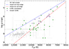 |
Fig. 1. Candidate stars in the Teff–log g plane. The positions of the candidate sample are shown as green squares in the Teff–log g plane. The known ZZ Ceti (Romero et al. 2022) and ELMVs (Hermes et al. 2012, 2013a,b; Kilic et al. 2015; Bell et al. 2015, 2017; Pelisoli et al. 2018a; Lopez et al. 2021) are shown as grey dots and purple diamonds, respectively. The ELMV found by Guidry et al. (2021) is not depicted since its atmospheric parameters have not been determined. The empirical ZZ Ceti instability strip published in Gianninas et al. (2015) is marked with dashed lines. |
3. Observations
3.1. High speed photometry
High-speed time-series photometry was obtained using Goodman spectrograph at the 4.1 m Southern Astrophysical Research (SOAR) Telescope and the Small and Moderate Aperture Research Telescope System (SMARTS) 1 metre telescope. With Goodman/SOAR we used the Blue Camera with the S8612 red-blocking filter. We used read-out mode 200 Hz ATTN2 with the CCD binned 2 × 2 and integration time ranging from 4 to 80 seconds, depending on each star’s magnitude and weather conditions, and with about 6 s dead time between each exposure. For SMARTS telescope we used Apogee F42 camera and the SDSSg filter, with the CCD binned 1 × 1 and integration time from 28 to 60 seconds, with about 4 s dead time. Further photometric observations details can be seen in Table A.1.
Both SOAR and SMARTS photometric data were reduced using the software IRAF, with the package DAOPHOT to perform aperture photometry. All photometry images were bias-subtracted, and flat field corrected using dome flats. Neighbouring non-variable stars of similar brightness were used as comparison stars to perform the differential photometry. We then divided the light curve of the target star by the mean light curve of all comparison stars to minimise the effects of sky and transparency fluctuations.
3.2. Spectroscopy
The ongoing characterisation of ELM candidates is being carried out with multiple telescope and instruments to ensure all-sky coverage. Five out of the 16 stars in this work have SDSS spectra (from the original SDSS spectrograph). Six were observed with the Goodman spectrograph (Clemens et al. 2004) at SOAR, four with the Intermediate Dispersion Spectrograph (IDS) installed at the 2.54 m Isaac Newton Telescope (INT), and the remaining one was observed with the Gemini Multi-Object Spectrographs (GMOS) at the 8 m Gemini South telescope (Hook et al. 2004; Gimeno et al. 2016). Details about the configuration at each telescope are given in Table A.2. For all observations, we aimed to cover the optical range, in particular the region of high-order Balmer lines, which is sensitive to log g in the low-mass range, and the slit width was set to be comparable to the seeing.
All the data were reduced using IRAF. We performed bias subtraction and flat-field correction using internal flat lamps. Arc lamp spectra for wavelength calibration were taken for every observation with the same pointing to minimise flexure effects. Flux calibration was performed with a standard star observed with the same setup. Due to slit losses, the flux calibration is not absolute but it does correct for the instrument response.
4. Methods
4.1. Light curve analysis: looking for periodicities
To look for periodicities in the light curves due to pulsations, we calculated the Fourier transform (FT) using the software Period04 (Lenz & Breger 2004). We accepted a frequency peak as significant if its amplitude exceeds an adopted significance threshold. In this work, the detection limit (e.g. dashed line in Fig. 2) corresponds to 1/1000 of the false alarm probability (FAP); any peak with an amplitude above this value has a 0.1% probability of being a false detection due to noise. The FAP was calculated by shuffling the fluxes in the light curve while keeping the same time sampling and computing the FT of the randomised data. This procedure was repeated N/2 times, where N is the number of points in the light curve. For each run, we computed the maximum amplitude of the FT. From the distribution of maxima, we took the 0.999 percentile as the detection limit (Romero et al. 2020). Also, for each new FT and light curve after each pre-whitening process, we calculated a new value for the FAP. The internal uncertainties in frequency and amplitude were computed using a Monte Carlo method with 100 simulations with PERIOD04, while uncertainties in the periods were obtained through error propagation.
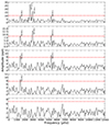 |
Fig. 2. Pre-whitening process for the star SDSS J090559.60+084324.9. All real peaks above the detection threshold (depicted as the dashed red line) were subtracted until only the noise from the FT remained. |
4.2. Spectroscopic fit
The spectra were fitted in the range 3800–5000 Å using a pure-hydrogen atmosphere grid similar to that used in Kepler et al. (2021), with the log g range extended down to 4.0. For each observed spectrum, we calculated a χ2 with every model in the grid, first broadening the models to the resolution of the observations, and applying an extinction-correction to the observed spectrum using the AV values of Lallement et al. (2019) at each target’s Gaia-derived distance and Fitzpatrick & Massa (2007)’s extinction law. The spectra and models were normalised by a constant free parameter, preserving the slope of the observations but not the absolute flux, given potential slit losses. The radial velocity (RV) was also left as a free parameter. This resulted in an absolute minimum for the majority of targets (see an example in Fig. 3), with a few exceptions where there were two possible solutions. In these cases, we ran a Markov chain Monte Carlo (MCMC) fit with the same free parameters, but placing a prior on the effective temperature to make it consistent with the temperature derived from a spectral energy distribution (SED) fit to the SDSS and Gaia magnitudes (see an example fit in Fig. 4). Uncertainties were determined from the 68% confidence interval of the χ2-determined likelihood for the χ2 fits, or from the posterior distribution in the MCMC fits. The results of the fits are reported in Table A.3, and the fits not shown in the main text are in Figs. D.1 (MCMC fit) and D.2 (χ2 fit). In some cases, the reduced χ2 of the fit is high (≳50); that is a consequence of one of two scenarios: (i) the presence of metals, which remain in the atmosphere of low-mass WDs for longer due to rotational mixing (Istrate et al. 2016), or (ii) the presence of an unseen companion contributing significantly to the flux. When metals are present, there is an additional systematic uncertainty of up to 1 dex in log g (see Pelisoli et al. 2018b). The presence of a companion is inferred either from the presence of extra light in the spectrum, which we see as a spectral slope that cannot be described by the models (J0159–1805, J0406–5427, and J1832+1413), or from a mismatch between the spectral slope and width of the spectral lines (J1346–1350 and J2129). The former is more likely caused by a companion with a different colour, whereas the latter by a companion with a similar colour that only dilutes the absorption lines. Determining the exact nature of the companion would require either greater spectral coverage, as spectra for the systems showing indication of a companion do not extend beyond ∼5000 Å, or RV monitoring. As neither metals nor the dilution by a companion are taken into account here, the reported values in Table A.3 should be interpreted with caution, but serve their purpose of identifying potential systems in the instability strip for follow-up.
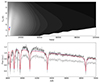 |
Fig. 3. Spectroscopic fit of J183702.03–674141.1. Top: χ2 as a function of Teff and log g. The blue dot indicates the absolute minimum. The red error bar shows the median (marked by a cross) and 68% confidence interval. Bottom: Observed spectrum (light grey), the extinction-corrected spectrum (darker grey), the model for minimum χ2 (blue), and the adopted solution (red). Note that this object has atmospheric metals that are not included in the model. |
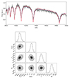 |
Fig. 4. Spectroscopic fit of J151626.39–265836.9. Top: Observed spectrum (light grey), the extinction-corrected spectrum (darker grey; with large overlap due to low extinction), the model for minimum χ2 (blue), and the adopted solution (red). Bottom: Corner plot for the MCMC fit. ‘RV’ is the radial velocity in km/s, and ‘μ’ is the constant normalisation parameter. |
5. Results
We report the discovery of three new pulsating WDs: one potential pulsating ELM WD (an ELMV), one low-mass WD, and one ZZ Ceti star (all of which are discussed further in Sect. 5.1). Additionally, in our search for variability, we identified three stars in binary systems. Among these, two exhibit ellipsoidal variations; one of these is likely a pre-ELM star, while the third shows reflection effects (see Sect. 5.2). Detailed information on the effective temperatures, surface gravity, masses, and types of variations for these targets is provided in Table A.3. Furthermore, we observed no detectable variability in the ten other stars in our sample (see Sect. 5.3).
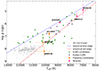 |
Fig. 5. Teff–log g plane depicting the position of the three new pulsating WDs, shown as orange × symbols, and the three new binary systems, shown as pink + signs. All values for Teff and log g for these six new variable objects are those calculated in this work. The known ZZ Ceti (Romero et al. 2022) and ELMVs (Hermes et al. 2012, 2013a,b; Kilic et al. 2015; Bell et al. 2015, 2017; Pelisoli et al. 2018a; Lopez et al. 2021) are shown as black dots and purple diamonds, respectively. The empirical ZZ Ceti instability strip published in Gianninas et al. (2015) is marked with dashed lines. |
5.1. New pulsating white dwarfs
5.1.1. SDSS J212935.23+001332.3
SDSS J212935.23+001332.3, with a magnitude of G = 15.54 and located at a Gaia-derived distance of 1/parallax = 65.4 ± 0.2 pc, was observed on three separate nights with the SOAR telescope and once with the SMARTS 1 m telescope, resulting in a total of approximately 9.5 hours of observations. Due to intermittent cloudy conditions on some nights, not all data could be used. To ensure the accuracy of our final analysis, only observations from nights with clear conditions were included for a thorough FT analysis.
Our spectral fitting of the observed INT spectra yields an Teff of 9700 K, log g = 6.8 ± 0.2 consistent within 2.4σ with the values reported by Caron et al. (2023) of Teff = 8860 ± 30 K, log g = 7.16 ± 0.006, along with a measured mass of 0.244 ± 0.002 M⊙ for the same star (see Fig. C.1). The spectrum also shows indications of potential excess light that could originate from a binary companion. However, further spectral observations and RV measurements are required to confirm the binary nature of this object.
Figure 6 displays the phase-folded light curves from one of the SOAR nights (top panel) and the SMARTS night (bottom panel), with sinusoidal fits indicated by the red lines. Due to unstable weather conditions, a lower S/N, and the longer cadence of the SMARTS observations, the SMARTS light curve does not clearly exhibit the sinusoidal pattern visible in the SOAR light curve, as shown in the same figure.
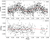 |
Fig. 6. Phased-folded light curve for the new ELMV SDSS J212935.23+001332.3 from the first observing night with SOAR (top) and SMARTS–1 m (bottom). Both light curves were folded to the highest-amplitude pulsational period of about P = 1.22 hours. The red line indicates a sinusoidal fit and helps show the variation. |
The FT of the SOAR light curves is presented in Fig. 7. In this figure, the data from the second and fourth nights are shown in the top and middle panels, respectively, while the bottom panel displays the combined data from these two nights. Unfortunately, the unstable cloud conditions during the first and third SOAR nights, as well during the night of observations with SMARTS, prevented a reliable analysis of the pulsation peaks in the FT, and thus their data are not included here. The horizontal dashed red line in all panels of Fig. 7 indicates our threshold for FAP of 1/1000.
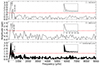 |
Fig. 7. FT for the new ELMV SDSS J212935.23+001332.3. The second and fourth observed SOAR nights are shown in the top and middle panels, respectively, while the combined data from the two nights are displayed in the bottom panel. The amplitude at the FAP = 1/1000 detection limit in each case is indicated by the horizontal dashed red line, and the spectral window for each case is depicted as an inset plot. |
Our analysis identified two prominent peaks above FAP = 1/1000 threshold in the FT, corresponding to periods of approximately 1.22 hours and 42 minutes. These periods are highly consistent with the typical pulsation periods of ELMVs, which range from 200 s to 7000 s (Córsico & Althaus 2016; Istrate et al. 2016; Calcaferro et al. 2018). Details about these peaks are provided in Table 1. Furthermore, this star is placed close to the known ELMVs (see Fig. 5) in the Teff–log g plane, combined with the calculated mass 0.244 M⊙ (Caron et al. 2023). The combination of the pulsation periods, observed in this object, characteristic of ELMVs, and the Teff and log g values determined in this work, suggests that this object is a compelling new addition to the known population of pulsating ELM WDs.
Detected frequencies for the new ELMV SDSS J212935.23+001332.3.
As shown in Fig. 5, SDSS J212935.23+001332.3 is located within the instability strip and close to the known ELMVs.
5.1.2. SDSS J001245.60+143956.4
SDSS J001245.60+143956.4 was observed during 3.4hrs with SOAR. With a magnitude of G = 18.19 and a Gaia-derived distance of 1/parallax = 359 ± 24 pc, this object has also an SDSS spectrum available. Our spectral fitting gives us Teff = 10 200 K and log g = 7.5 ± 0.4, which is perfectly consistent with the existing solution from Kleinman et al. (2013), who estimated Teff = 10893 ± 68K, log g = 7.74 ± 0.07, and a mass of 0.482 ± 0.03 M⊙ (see Fig. C.1). For this object the measured Teff and log g agree with each other within uncertainties, and Kleinman et al. (2013) delivered mass places this objects as a low-mass WD.
In Fig. 8 (top panel) we show the folded light curve with the period of P = 347 s for the SOAR night as well as its FT (bottom panel). Our analysis shows five peaks above our threshold, the highest-amplitude peak corresponding to a period of about 347 seconds (see details in Table 2). The pulsation periods observed for this object are also consistent with the typical pulsation periods of low-mass WDs. For comparison, a pulsating low-mass WD identified by Parsons et al. (2020) within a binary system, SDSS J115219.99–024814.4, exhibits pulsation periods ranging from 1314 s to 582 s. Although the WD observed by Parsons et al. (2020) has a lower measured mass (0.325 ± 0.013 M⊙) compared to the object analysed in this work (0.482 ± 0.03 M⊙), the observed pulsation periods fall within the expected range for low-mass WDs (Córsico & Althaus 2016; Calcaferro et al. 2018).
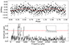 |
Fig. 8. Light Curve and Fourier Transform of SDSS J001245.60+143956.4. Top: Phased-folded light curve for the new pulsating low-mass WD SDSS J001245.60+143956.4. The light curve was folded to the highest-amplitude pulsational period of about P = 347 s. The solid red line indicates a sinusoidal fit, depicted for a better visualisation of the variation. Bottom: FT for the same star. The horizontal dashed red line indicates our detection limit, and the spectral window for each case is depicted as an inset plot. |
Detected frequencies for the new pulsating low-mass WD SDSS J001245.60+143956.4.
Furthermore, the location of this objects within Teff–log g plane (see Fig. 5) also places this objects within the instability strip.
5.1.3. SDSS J090559.60+084324.9
SDSS J090559.60+084324.9 is the third pulsational object discovered in this work. It has a magnitude of G = 18.00 and is located at a Gaia-derived distance of 1/parallax = 245 ± 8 pc. This star was observed for 2.11 hs with the SOAR telescope; four periodical peaks were observed above the threshold (see the bottom panel of Fig. 9, and the details of each peak found can be seen on Table 3). This star has also an SDSS spectrum available and our spectral fit has retrieved atmospheric parameters of Teff = 10 100 K and log g = 8.2 ± 0.4. Once more, our spectral fit is in perfect agreement with the work done by Kleinman et al. (2013), who measured Teff = 10 070.0 ± 38, log g = 8.18 ± 0.04, and a mass of 0.704 ± 0.03 M⊙ (see Fig. C.1). Those values identified this star as a typical ZZ Ceti.
Detected frequencies for the new ZZ Ceti SDSS J090559.60+084324.9.
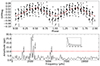 |
Fig. 9. Light Curve and Fourier Transform of SDSS J090559.60+084324.9. Top: Phased-folded light curve for the new ZZ Ceti SDSS J090559.60+084324.9. The light curve was folded to the highest-amplitude pulsational period of about P = 377 s. The solid red line indicates a sinusoidal fit, depicted for a better visualisation of the variation. The ‘lined’ appearance in the folded light curve is attributed to the 337 s pulsation period being close to an alias of the cadence. Bottom: FT for the same star. The horizontal dashed red line indicates our detection limit, and the spectral window is depicted as an inset plot. |
For this object in particular, it was not surprising that we identified a ZZ Ceti star. In our candidate selection process, we accounted for the uncertainties in Teff and log g, which were considerable in many cases. Additionally, we extended our search to include slightly higher Teff and log g values. This approach was motivated by the fact that the instability strips of ZZ Ceti and ELMV stars are a continuation of each other, with no clearly defined boundaries separating the two groups to date.
Nevertheless, the atmospheric parameters derived in this work place this new ZZ Ceti slightly outside the red edge of the instability strip. (see Fig. 5), towards the red edge. However, the star’s location is still close to the positions of other known ZZ Ceti stars.
5.2. New binary white dwarfs
5.2.1. SDSS J045116.83+010426.6
SDSS J045116.83+010426.6 has a magnitude of G = 15.35 and is located at a Gaia-derived distance of 1/parallax = 294 ± 3 pc. This star was observed on two different nights with SOAR; both light curves showed strong variations, as seen in the phased-folded light curve in the top panel of Fig. 10 for just one of the SOAR nights. This variation in the light curve appears to show an ellipsoidal variation, presumably due to the gravitational deformation of one of the two stars (Barlow et al. 2022). Also, the significant difference between the minima in the light curve is striking and suggests that additional data, particularly in other filters, could provide insight into its origin.
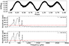 |
Fig. 10. Light Curve and Fourier Transform of SDSS J045116.83+010426.6. Top: SDSS J045116.83+010426.6 phased-folded light curve to Porb = 1.35 h, which is twice the period of the peak with the highest amplitude in the FT. Middle and bottom: FTs for two different SOAR nights. The horizontal dashed red line for both FTs indicates our detection limit. |
We estimate the orbital period to be Porb = 1.35 h for the combined nights, which is two times greater than the highest peak in both FT (middle and bottom panel) in Fig. 10. The ∼26 min peak that appears in both periodograms of Fig. 10, is a combination of the ∼1.4 h and ∼40 min peaks.
For this object we carried out spectroscopic observations with the INT, which revealed a rich spectrum with strong metal lines. Furthermore, a preliminary SED and the co-added spectrum, which reveals a significant presence of metals (as shown in Fig. D.2), suggest a primary star consistent with a pre-ELM, with Teff = 7000 K and log g = 4.9 ± 0.5.
A spectrum with higher signal-to-noise ratio (S/N) and higher resolution will be necessary to confirm the system orbital period with RV measurements, to fully confirm the primary star nature, and to determine the nature of the secondary companion.
5.2.2. SDSS J183245.52+141311.2
SDSS J183245.52+141311.2 has been observed during only one night with SOAR, and it has a magnitude of G = 17.45 and 1/parallax = 1503 ± 207 pc. The light curve of this object has shown a strong sinusoidal variation with an amplitude of about ∼0.05 mag (see the top panel of Fig. 11). The FT (bottom panel of Fig. 11) depict a strong peak of P = 2.58 h. The high-amplitude variation in its light curve, and its detected period is very characteristic for reflection effect, in which it originates from the irradiation of a cool companion by the hot primary star. The projected area of the companion’s heated hemisphere changes while it orbits the primary. Our spectral fit indicates that the primary star has (Teff = 8860 ± 100 K and log g = 5.9 ± 0.1. The spectroscopic fit indicates the presence of additional light, suggesting a cooler companion, as evidenced by the slope of the spectrum shown in Fig. D.2. This interpretation aligns with the observed reflection effect in the system. However, the wavelength range of our spectra does not extend far enough into the red to reveal distinct features of a potential M dwarf. Consequently, we cannot rule out the possibility of a cool WD, a brown dwarf, or an M dwarf as a companion. Further spectroscopic follow-up is needed to obtain RV measurements, which in turn are necessary to confirm the binary nature of this object, and to detect the nature of the secondary star.
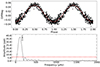 |
Fig. 11. Light Curve and Fourier Transform of SDSS J183245.52+141311.2. Top: SDSS J183245.52+141311.2 phased-folded light curve to Porb = 2.58 h, showing a strong reflection effect. The solid red line indicates a sinusoidal fit, depicted for a better visualisation of the variation. Bottom: FT with a high-amplitude peak high above our detection limit. The detection limit is indicated by the dashed red line. |
5.2.3. SDSS J083417.21–652423.2
SDSS J083417.21–652423.2, G = 16.77 and 1/parallax = 790 ± 27 pc, was observed with SOAR on just one nigh; we estimate its orbital period to be P = 2.32 h. The object light curve, shown in the top panel in Fig. 12, exhibits a characteristic, quasi-sinusoidal shape in which the flux peaks are slightly sharper than the valleys.
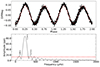 |
Fig. 12. Light Curve and Fourier Transform of SDSS J083417.21–652423.2. Top: SDSS J083417.21–652423.2 phased-folded light curve, showing the ellipsoidal variation, to Porb = 2.32 h, which is twice the period of the peak with the highest amplitude in the FT. The solid red line indicates a sinusoidal fit, depicted for a better visualisation of the variation. Bottom: FT. The horizontal dashed red line indicates our detection limit. |
Similar to the case of SDSS J045116.83+010426.6 (see Sect. 5.2.1), the highest-amplitude peak in the FT (bottom panel in Fig. 12) represents half of the orbital period; one can clearly see the difference in two consecutive peaks and valleys in the folded light curve (top panel in Fig. 12) once we fold the light curve to twice the period of the main highest peak. The consecutive troughs and crests are uneven, which is likely due to a combination of effects, such as ellipsoidal modulation, gravity darkening, and reflection effects (Barlow et al. 2022).
Our spectral fit yielded  K and log g = 4.9 ± 0.5. However, further observations with higher S/N and resolution are needed to better constrain the atmospheric parameters and RV measurements, and to confirm the orbital period of the system.
5.3. Non observed to vary (NOV)
From the observed sample, we do not detect any variability in the FT for ten objects, within our detection limit (see Table B.1), and thus they are classified as not observed to vary (NOV). We list the objects in Table A.3, and their light curves and periodogram can be seen in Figs. B.1 and B.2, respectively. Since the low-mass and ELM instability strip is possibly not pure, we might have objects that fall within the instability strip and have no pulsational variability, and we might have estimated atmospheric parameters incorrectly. Furthermore, we recommend follow-up observations for those objects given the low amplitude of the ELM pulsations, which makes it challenging to detect pulsations in those objects.
6. Summary and conclusions
Via our comprehensive analysis, we identified 16 objects from high-speed photometry across multiple nights using the SOAR/Goodman and SMARTS-1 m telescopes. This led to the detection of three new pulsating WDs: a new pulsating ELM WD (an ELMV), a low-mass WD, and a ZZ Ceti star.
-
SDSS J212935.23+001332.3 is identified as a potential new pulsating ELM WD, with prominent pulsation periods of 1.22 hours and 42 minutes. Our spectral fitting of the observed INT spectra yields an Teff of 9700
 K and log g = 6.8 ± 0.2, which places this object close to known ELMVs in the Teff–log g plane. Based on this plus its measured mass of 0.244 ± 0.002 M⊙ (Caron et al. 2023), we classify this object as new pulsating ELM WD. Further detailed spectroscopic analysis and asteroseismology analysis would be necessary to further confirm its ELMV nature since the spectroscopical fit suggests additional light.
 -
SDSS J001245.60+143956.4 exhibits pulsations with a dominant period of around 347 seconds. Our spectral fitting results, Teff = 10 200
 K and log g = 7.5 ± 0.4, and its measured mass of 0.482 ± 0.03 M⊙ (Kleinman et al. 2013) place the star within the instability strip for ZZ Ceti and ELMV WDs, and we classify this star as a new pulsating low-mass WD.
 -
SDSS J090559.60+084324.9 is a new confirmed ZZ Ceti star with four observed pulsational periods. The star lies near the red edge of the ZZ Ceti instability strip, with Teff = 10 100
 K and log g = 8.2 ± 0.4. These measurements along with a measured mass of 0.704 ± 0.03 M⊙ (Kleinman et al. 2013) are consistent with characteristics of a typical ZZ Ceti.
In addition, three new binary systems were discovered, two of which exhibit ellipsoidal variations due to gravitational deformation; the third shows reflection effects from a heated companion. Our spectral analyses provide insights into the primary stars in these systems, but further follow-up, including RV measurements, is needed to confirm the nature of the companions.
-
SDSS J045116.83+010426.6 shows in its light curves strong ellipsoidal variations that are presumably due to the gravitational deformation of one of the two stars. The estimated orbital period is 1.35 hours. A preliminary SED and a co-added spectrum fit suggest that the primary star is a pre-ELM WD (Teff =
 K, and log g = 4.9 ± 0.5).
 -
The SDSS J183245.52+141311.2 light curve exhibits a strong sinusoidal variation, likely due to a reflection effect from a cool companion being irradiated by a hot primary. The estimated orbital period is 2.58 hours, and the derived atmospheric parameters of Teff = 8860 ± 100 K and log g = 5.9 ± 0.1 suggest that the primary star is a WD. However, further spectroscopic follow-up is needed to confirm the binary nature and the secondary star’s properties.
-
The SDSS J083417.21–652423.2 light curve suggests ellipsoidal variations, and the uneven peaks and valleys indicate gravity-darkening and Doppler beaming effects. Our analysis returns a potential orbital period of 2.32 hours,
 K, and log g = 4.9 ± 0.5. Higher-quality data are needed to refine the orbital parameters and confirm the system’s details.
Finally, the ten other stars in the sample showed no detectable variability. While these objects fall within potential instability strips, they did not exhibit pulsations during the observation period. The absence of variability in these cases could be due to low-amplitude pulsations or inaccuracies in the atmospheric parameter estimates. Follow-up observations are recommended, as the detection of low-amplitude pulsations may have been hindered.
Acknowledgments
LAA acknowledges financial support from CONICYT Doctorado Nacional in the form of grant number No: 21201762 and ESO studentship program. MV acknowledges the financial support from the FONDECYT Regular Grant No 1211941. IP acknowledges support from The Royal Society through a University Research Fellowship (URF/R1/231496). Based on observations collected with the GMOS spectrograph on the 8.1 m Gemini-South telescope at Cerro Pachón, Chile, under the program GS-2022A-Q-416, and observation with Goodman SOAR 4.1 m telescope, at Cerro Pachón, Chile, and SMARTS-1 m telescope at Cerro Tololo, Chile, under the program allocated by the Chilean Time Allocation Committee (CNTAC), no: CN2022A-412490, and SOAR observational time through NOAO programs 2021A-XXXX. M.V. acknowledges support from FONDECYT (grant No: 1211941).
References
- Aerts, C., Christensen-Dalsgaard, J., & Kurtz, D. W. 2010, Asteroseismology (Springer Science+Business Media B.V.) [Google Scholar]
- Althaus, L. G., Miller Bertolami, M. M., & Córsico, A. H. 2013, A&A, 557, A19 [NASA ADS] [CrossRef] [EDP Sciences] [Google Scholar]
- Amaro-Seoane, P., Audley, H., Babak, S., et al. 2017, arXiv e-prints [arXiv:1702.00786] [Google Scholar]
- Barlow, B. N., Corcoran, K. A., Parker, I. M., et al. 2022, ApJ, 928, 20 [NASA ADS] [CrossRef] [Google Scholar]
- Bell, K. J., Kepler, S. O., Montgomery, M. H., et al. 2015, in 19th European Workshop on White Dwarfs, Proceedings of a conference held at the Université de Montréal, Montréal, Canada, 11-15 August 2014, eds. P. Dufour, P. Bergeron, & G. Fontaine (San Francisco, CA, USA: Astronomical Society of the Pacific), Astronomical Society of the Pacific Conference Series, 493, 217 [Google Scholar]
- Bell, K. J., Gianninas, A., Hermes, J. J., et al. 2017, ApJ, 835, 180 [Google Scholar]
- Bell, K. J., Hermes, J. J., & Kuszlewicz, J. S. 2018, arXiv e-prints [arXiv:1809.05623] [Google Scholar]
- Bildsten, L., Shen, K. J., Weinberg, N. N., & Nelemans, G. 2007, ApJ, 662, L95 [Google Scholar]
- Blanton, M. R., Bershady, M. A., Abolfathi, B., et al. 2017, AJ, 154, 28 [Google Scholar]
- Boubert, D., Strader, J., Aguado, D., et al. 2019, MNRAS, 486, 2618 [Google Scholar]
- Brown, W. R., Kilic, M., Allende Prieto, C., & Kenyon, S. J. 2010, ApJ, 723, 1072 [Google Scholar]
- Brown, W. R., Gianninas, A., Kilic, M., Kenyon, S. J., & Allende Prieto, C. 2016, ApJ, 818, 155 [Google Scholar]
- Brown, W. R., Kilic, M., Kosakowski, A., & Gianninas, A. 2022, ApJ, 933, 94 [NASA ADS] [CrossRef] [Google Scholar]
- Brown, A. J., Parsons, S. G., van Roestel, J., et al. 2023, MNRAS, 521, 1880 [NASA ADS] [CrossRef] [Google Scholar]
- Calcaferro, L. M., Córsico, A. H., Althaus, L. G., Romero, A. D., & Kepler, S. O. 2018, A&A, 620, A196 [EDP Sciences] [Google Scholar]
- Caron, A., Bergeron, P., Blouin, S., & Leggett, S. K. 2023, MNRAS, 519, 4529 [NASA ADS] [CrossRef] [Google Scholar]
- Clemens, J. C., Crain, J. A., & Anderson, R. 2004, in Ground-based Instrumentation for Astronomy, eds. A. F. M. Moorwood, & M. Iye (Bellingham, WA, USA: SPIE), Society of Photo-Optical Instrumentation Engineers (SPIE) Conference Series, 5492, 331 [NASA ADS] [CrossRef] [Google Scholar]
- Córsico, A. H., & Althaus, L. G. 2014, A&A, 569, A106 [NASA ADS] [CrossRef] [EDP Sciences] [Google Scholar]
- Córsico, A. H., & Althaus, L. G. 2016, A&A, 585, A1 [NASA ADS] [CrossRef] [EDP Sciences] [Google Scholar]
- Córsico, A. H., Romero, A. D., Althaus, L. G., & Hermes, J. J. 2012, A&A, 547, A96 [NASA ADS] [CrossRef] [EDP Sciences] [Google Scholar]
- Fitzpatrick, E. L., & Massa, D. 2007, ApJ, 663, 320 [Google Scholar]
- Fontaine, G., & Brassard, P. 2008, PASP, 120, 1043 [NASA ADS] [CrossRef] [Google Scholar]
- Gianninas, A., Kilic, M., Brown, W. R., Canton, P., & Kenyon, S. J. 2015, ApJ, 812, 167 [Google Scholar]
- Gimeno, G., Roth, K., Chiboucas, K., et al. 2016, in Ground-based and Airborne Instrumentation for Astronomy VI, eds. C. J. Evans, L. Simard, & H. Takami (Bellingham, WA, USA: SPIE), Society of Photo-Optical Instrumentation Engineers (SPIE) Conference Series, 9908, 99082S [NASA ADS] [Google Scholar]
- Guidry, J. A., Vanderbosch, Z. P., Hermes, J. J., et al. 2021, ApJ, 912, 125 [NASA ADS] [CrossRef] [Google Scholar]
- Hermes, J. J., Montgomery, M. H., Winget, D. E., et al. 2012, ApJ, 750, L28 [Google Scholar]
- Hermes, J. J., Montgomery, M. H., Winget, D. E., et al. 2013a, in 18th European White Dwarf Workshop, Proceedings of a conference held 13-17 August, 2012, at the Pedagogical University of Cracow, Poland, eds. J. Krzesiński, G. Stachowski, P. Moskalik, & K. Bajan (San Francisco, CA, USA: Astronomical Society of the Pacific), Astronomical Society of the Pacific Conference Series, 469, 57 [Google Scholar]
- Hermes, J. J., Montgomery, M. H., Gianninas, A., et al. 2013b, MNRAS, 436, 3573 [Google Scholar]
- Hook, I. M., Jørgensen, I., Allington-Smith, J. R., et al. 2004, PASP, 116, 425 [NASA ADS] [CrossRef] [Google Scholar]
- Iben, I., Jr., & Livio, M. 1993, PASP, 105, 1373 [CrossRef] [Google Scholar]
- Iben, I., Jr., & Tutukov, A. V. 1984, ApJS, 54, 335 [NASA ADS] [CrossRef] [Google Scholar]
- Iben, I., Jr., & Tutukov, A. V. 1986, ApJ, 311, 753 [NASA ADS] [CrossRef] [Google Scholar]
- Istrate, A. G., Marchant, P., Tauris, T. M., et al. 2016, A&A, 595, A35 [NASA ADS] [CrossRef] [EDP Sciences] [Google Scholar]
- Kepler, S. O., Koester, D., Romero, A. D., Ourique, G., & Pelisoli, I. 2017, in 20th European White Dwarf Workshop, Proceedings of a conference held at the University of Warwick, Coventry, West Midlands, United Kingdom, 25-29 July 2016, eds. P. E. Tremblay, B. Gänsicke, & T. Marsh (San Francisco, CA, USA: Astronomical Society of the Pacific), Astronomical Society of the Pacific Conference Series, 509, 421 [Google Scholar]
- Kepler, S. O., Koester, D., Pelisoli, I., Romero, A. D., & Ourique, G. 2021, MNRAS, 507, 4646 [NASA ADS] [CrossRef] [Google Scholar]
- Kilic, M., Hermes, J. J., Gianninas, A., & Brown, W. R. 2015, MNRAS, 446, L26 [Google Scholar]
- Kleinman, S. J., Kepler, S. O., Koester, D., et al. 2013, ApJS, 204, 5 [NASA ADS] [CrossRef] [Google Scholar]
- Kosakowski, A., Brown, W. R., Kilic, M., et al. 2023, ApJ, 950, 141 [CrossRef] [Google Scholar]
- Lallement, R., Babusiaux, C., Vergely, J. L., et al. 2019, A&A, 625, A135 [NASA ADS] [CrossRef] [EDP Sciences] [Google Scholar]
- Lauffer, G. R., Romero, A. D., & Kepler, S. O. 2018, MNRAS, 480, 1547 [NASA ADS] [CrossRef] [Google Scholar]
- Lenz, P., & Breger, M. 2004, in The A-Star Puzzle, eds. J. Zverko, J. Ziznovsky, S. J. Adelman, & W. W. Weiss, 224, 786 [Google Scholar]
- Li, Z., Chen, X., Chen, H.-L., & Han, Z. 2019, ApJ, 871, 148 [NASA ADS] [CrossRef] [Google Scholar]
- Lindegren, L., Hernández, J., Bombrun, A., et al. 2018, A&A, 616, A2 [NASA ADS] [CrossRef] [EDP Sciences] [Google Scholar]
- Lopez, I. D., Hermes, J. J., Calcaferro, L. M., et al. 2021, ApJ, 922, 220 [NASA ADS] [CrossRef] [Google Scholar]
- Marsh, T. R., Dhillon, V. S., & Duck, S. R. 1995, MNRAS, 275, 828 [Google Scholar]
- Nelemans, G., Portegies Zwart, S. F., Verbunt, F., & Yungelson, L. R. 2001, A&A, 368, 939 [NASA ADS] [CrossRef] [EDP Sciences] [Google Scholar]
- Paczynski, B. 1976, in Structure and Evolution of Close Binary Systems, eds. P. Eggleton, S. Mitton, & J. Whelan, 73, 75 [NASA ADS] [CrossRef] [Google Scholar]
- Parsons, S. G., Gänsicke, B. T., Marsh, T. R., et al. 2017, MNRAS, 470, 4473 [Google Scholar]
- Parsons, S. G., Brown, A. J., Littlefair, S. P., et al. 2020, Nat. Astron., 4, 690 [Google Scholar]
- Pelisoli, I., & Vos, J. 2019, MNRAS, 488, 2892 [Google Scholar]
- Pelisoli, I., Kepler, S. O., Koester, D., et al. 2018a, MNRAS, 478, 867 [Google Scholar]
- Pelisoli, I., Kepler, S. O., & Koester, D. 2018b, MNRAS, 475, 2480 [NASA ADS] [CrossRef] [Google Scholar]
- Pyrzas, S., Gänsicke, B. T., Hermes, J. J., et al. 2015, MNRAS, 447, 691 [Google Scholar]
- Romero, A. D., Antunes Amaral, L., Kepler, S. O., et al. 2020, MNRAS, 497, L24 [Google Scholar]
- Romero, A. D., Kepler, S. O., Hermes, J. J., et al. 2022, MNRAS, 511, 1574 [NASA ADS] [CrossRef] [Google Scholar]
- Steinfadt, J. D. R., Bildsten, L., & Arras, P. 2010, ApJ, 718, 441 [Google Scholar]
- Tremblay, P. E., Cummings, J., Kalirai, J. S., et al. 2016, MNRAS, 461, 2100 [NASA ADS] [CrossRef] [Google Scholar]
- Van Grootel, V., Fontaine, G., Brassard, P., & Dupret, M. A. 2013, ApJ, 762, 57 [NASA ADS] [CrossRef] [Google Scholar]
- Wang, K., Németh, P., Luo, Y., et al. 2022, ApJ, 936, 5 [CrossRef] [Google Scholar]
- Webbink, R. F. 1984, ApJ, 277, 355 [NASA ADS] [CrossRef] [Google Scholar]
- Winget, D. E., & Kepler, S. O. 2008, ARA&A, 46, 157 [Google Scholar]
- Zenati, Y., Toonen, S., & Perets, H. B. 2019, MNRAS, 482, 1135 [NASA ADS] [CrossRef] [Google Scholar]
- Zorotovic, M., & Schreiber, M. R. 2017, MNRAS, 466, L63 [CrossRef] [Google Scholar]
Appendix A: Details of the photometric and spectroscopic observations
Photometric observations from ground-based facilities.
Details of the spectroscopic observations that contributed to this work.
The 16 objects presented in this work.
Appendix B: NOV: Extra information
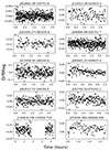 |
Fig. B.1. Light curve of the ten objects that were identified as NOV. |
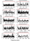 |
Fig. B.2. FT of the ten objects identified as NOV. Their respective FAP detection limit is depicted as a dashed red line. |
The ten objects identified as NOV.
Appendix C: Extra figures
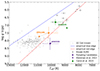 |
Fig. C.1. Teff − log g plane showing the positions of the three new pulsating WDs identified in this work, with atmospheric parameters from this study marked by × symbols. For comparison, atmospheric parameters from Kleinman et al. (2013) and Caron et al. (2023) are indicated by upside-down and right-side-up triangles, respectively. The known ZZ Ceti (Romero et al. 2022) and ELMVs (Hermes et al. 2012, 2013a,b; Kilic et al. 2015; Bell et al. 2015, 2017; Pelisoli et al. 2018a; Lopez et al. 2021) are shown as grey dots and grey diamonds, respectively. The empirical ZZ Ceti instability strip published in Gianninas et al. (2015) is marked with dashed lines. |
Appendix D: Full spectral fits
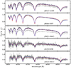 |
Fig. D.1. Spectral fits to objects that were fit using MCMC due to showing two minima in χ2. The observed spectrum is shown in light grey, the extinction-corrected spectrum in darker grey, the model for minimum χ2 in blue, and the adopted solution in red. |
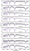 |
Fig. D.2. Spectral fits to objects with a single minimum in χ2. The observed spectrum is shown in light grey, the extinction-corrected spectrum in darker grey, the model for minimum χ2 in blue, and the adopted solution in red. |
All Tables
Detected frequencies for the new pulsating low-mass WD SDSS J001245.60+143956.4.
All Figures
|
Fig. 1. Candidate stars in the Teff–log g plane. The positions of the candidate sample are shown as green squares in the Teff–log g plane. The known ZZ Ceti (Romero et al. 2022) and ELMVs (Hermes et al. 2012, 2013a,b; Kilic et al. 2015; Bell et al. 2015, 2017; Pelisoli et al. 2018a; Lopez et al. 2021) are shown as grey dots and purple diamonds, respectively. The ELMV found by Guidry et al. (2021) is not depicted since its atmospheric parameters have not been determined. The empirical ZZ Ceti instability strip published in Gianninas et al. (2015) is marked with dashed lines. |
| In the text | |
|
Fig. 2. Pre-whitening process for the star SDSS J090559.60+084324.9. All real peaks above the detection threshold (depicted as the dashed red line) were subtracted until only the noise from the FT remained. |
| In the text | |
|
Fig. 3. Spectroscopic fit of J183702.03–674141.1. Top: χ2 as a function of Teff and log g. The blue dot indicates the absolute minimum. The red error bar shows the median (marked by a cross) and 68% confidence interval. Bottom: Observed spectrum (light grey), the extinction-corrected spectrum (darker grey), the model for minimum χ2 (blue), and the adopted solution (red). Note that this object has atmospheric metals that are not included in the model. |
| In the text | |
|
Fig. 4. Spectroscopic fit of J151626.39–265836.9. Top: Observed spectrum (light grey), the extinction-corrected spectrum (darker grey; with large overlap due to low extinction), the model for minimum χ2 (blue), and the adopted solution (red). Bottom: Corner plot for the MCMC fit. ‘RV’ is the radial velocity in km/s, and ‘μ’ is the constant normalisation parameter. |
| In the text | |
|
Fig. 5. Teff–log g plane depicting the position of the three new pulsating WDs, shown as orange × symbols, and the three new binary systems, shown as pink + signs. All values for Teff and log g for these six new variable objects are those calculated in this work. The known ZZ Ceti (Romero et al. 2022) and ELMVs (Hermes et al. 2012, 2013a,b; Kilic et al. 2015; Bell et al. 2015, 2017; Pelisoli et al. 2018a; Lopez et al. 2021) are shown as black dots and purple diamonds, respectively. The empirical ZZ Ceti instability strip published in Gianninas et al. (2015) is marked with dashed lines. |
| In the text | |
|
Fig. 6. Phased-folded light curve for the new ELMV SDSS J212935.23+001332.3 from the first observing night with SOAR (top) and SMARTS–1 m (bottom). Both light curves were folded to the highest-amplitude pulsational period of about P = 1.22 hours. The red line indicates a sinusoidal fit and helps show the variation. |
| In the text | |
|
Fig. 7. FT for the new ELMV SDSS J212935.23+001332.3. The second and fourth observed SOAR nights are shown in the top and middle panels, respectively, while the combined data from the two nights are displayed in the bottom panel. The amplitude at the FAP = 1/1000 detection limit in each case is indicated by the horizontal dashed red line, and the spectral window for each case is depicted as an inset plot. |
| In the text | |
|
Fig. 8. Light Curve and Fourier Transform of SDSS J001245.60+143956.4. Top: Phased-folded light curve for the new pulsating low-mass WD SDSS J001245.60+143956.4. The light curve was folded to the highest-amplitude pulsational period of about P = 347 s. The solid red line indicates a sinusoidal fit, depicted for a better visualisation of the variation. Bottom: FT for the same star. The horizontal dashed red line indicates our detection limit, and the spectral window for each case is depicted as an inset plot. |
| In the text | |
|
Fig. 9. Light Curve and Fourier Transform of SDSS J090559.60+084324.9. Top: Phased-folded light curve for the new ZZ Ceti SDSS J090559.60+084324.9. The light curve was folded to the highest-amplitude pulsational period of about P = 377 s. The solid red line indicates a sinusoidal fit, depicted for a better visualisation of the variation. The ‘lined’ appearance in the folded light curve is attributed to the 337 s pulsation period being close to an alias of the cadence. Bottom: FT for the same star. The horizontal dashed red line indicates our detection limit, and the spectral window is depicted as an inset plot. |
| In the text | |
|
Fig. 10. Light Curve and Fourier Transform of SDSS J045116.83+010426.6. Top: SDSS J045116.83+010426.6 phased-folded light curve to Porb = 1.35 h, which is twice the period of the peak with the highest amplitude in the FT. Middle and bottom: FTs for two different SOAR nights. The horizontal dashed red line for both FTs indicates our detection limit. |
| In the text | |
|
Fig. 11. Light Curve and Fourier Transform of SDSS J183245.52+141311.2. Top: SDSS J183245.52+141311.2 phased-folded light curve to Porb = 2.58 h, showing a strong reflection effect. The solid red line indicates a sinusoidal fit, depicted for a better visualisation of the variation. Bottom: FT with a high-amplitude peak high above our detection limit. The detection limit is indicated by the dashed red line. |
| In the text | |
|
Fig. 12. Light Curve and Fourier Transform of SDSS J083417.21–652423.2. Top: SDSS J083417.21–652423.2 phased-folded light curve, showing the ellipsoidal variation, to Porb = 2.32 h, which is twice the period of the peak with the highest amplitude in the FT. The solid red line indicates a sinusoidal fit, depicted for a better visualisation of the variation. Bottom: FT. The horizontal dashed red line indicates our detection limit. |
| In the text | |
|
Fig. B.1. Light curve of the ten objects that were identified as NOV. |
| In the text | |
|
Fig. B.2. FT of the ten objects identified as NOV. Their respective FAP detection limit is depicted as a dashed red line. |
| In the text | |
|
Fig. C.1. Teff − log g plane showing the positions of the three new pulsating WDs identified in this work, with atmospheric parameters from this study marked by × symbols. For comparison, atmospheric parameters from Kleinman et al. (2013) and Caron et al. (2023) are indicated by upside-down and right-side-up triangles, respectively. The known ZZ Ceti (Romero et al. 2022) and ELMVs (Hermes et al. 2012, 2013a,b; Kilic et al. 2015; Bell et al. 2015, 2017; Pelisoli et al. 2018a; Lopez et al. 2021) are shown as grey dots and grey diamonds, respectively. The empirical ZZ Ceti instability strip published in Gianninas et al. (2015) is marked with dashed lines. |
| In the text | |
|
Fig. D.1. Spectral fits to objects that were fit using MCMC due to showing two minima in χ2. The observed spectrum is shown in light grey, the extinction-corrected spectrum in darker grey, the model for minimum χ2 in blue, and the adopted solution in red. |
| In the text | |
|
Fig. D.2. Spectral fits to objects with a single minimum in χ2. The observed spectrum is shown in light grey, the extinction-corrected spectrum in darker grey, the model for minimum χ2 in blue, and the adopted solution in red. |
| In the text | |
Current usage metrics show cumulative count of Article Views (full-text article views including HTML views, PDF and ePub downloads, according to the available data) and Abstracts Views on Vision4Press platform.
Data correspond to usage on the plateform after 2015. The current usage metrics is available 48-96 hours after online publication and is updated daily on week days.
Initial download of the metrics may take a while.