| Issue |
A&A
Volume 685, May 2024
|
|
|---|---|---|
| Article Number | A9 | |
| Number of page(s) | 17 | |
| Section | Stellar structure and evolution | |
| DOI | https://doi.org/10.1051/0004-6361/202348564 | |
| Published online | 30 April 2024 | |
The double low-mass white dwarf eclipsing binary system J2102–4145 and its possible evolution
1
Instituto de Física y Astronomía, Universidad de Valparaíso, Gran Bretaña 1111, Playa Ancha, Valparaíso 2360102, Chile
e-mail: This email address is being protected from spambots. You need JavaScript enabled to view it.
2
European Southern Observatory, Alonso de Cordova 3107, Santiago, Chile
3
Department of Physics, University of Warwick, Gibbet Hill Road, Coventry CV4 7AL, UK
4
Isaac Newton Group of Telescopes, Apartado de Correos 368, 38700 Santa Cruz de La Palma, Spain
5
Astronomical Institute of the Czech Academy of Sciences, 251 65 Ondřejov, Czech Republic
6
Astroserver.org, Fő tér 1, 8533 Malomsok, Hungary
7
Department of Physics and Astronomy, University of Sheffield, Sheffield S3 7RH, UK
8
Instituto de Astrofísica de Canarias, 38205 La Laguna, Tenerife, Spain
Received:
10
November
2023
Accepted:
15
February
2024
Abstract
In recent years, about 150 low-mass white dwarfs (WDs), typically with masses below 0.4 M⊙, have been discovered. The majority of these low-mass WDs are observed in binary systems as they cannot be formed through single-star evolution within Hubble time. In this work, we present a comprehensive analysis of the double low-mass WD eclipsing binary system J2102−4145. Our investigation encompasses an extensive observational campaign, resulting in the acquisition of approximately 28 h of high-speed photometric data across multiple nights using NTT/ULTRACAM, SOAR/Goodman, and SMARTS-1m telescopes. These observations have provided critical insights into the orbital characteristics of this system, including parameters such as inclination and orbital period. To disentangle the binary components of J2102−4145, we employed the XTGRID spectral fitting method with GMOS/Gemini-South and X-shooter data. Additionally, we used the PHOEBE package for light curve analysis on NTT/ULTRACAM high-speed time-series photometry data to constrain the binary star properties. Our analysis unveils remarkable similarities between the two components of this binary system. For the primary star, we determine Teff,1 = 13 688−72+65 K, log g1 = 7.36 ± 0.01, R1 = 0.0211 ± 0.0002 R⊙, and M1 = 0.375 ± 0.003 M⊙, while, the secondary star is characterised by Teff,2 = 12952−66+53 K, log g2 = 7.32 ± 0.01, R2 = 0.0203−0.0003+0.0002 R⊙, and M2 = 0.314 ± 0.003 M⊙. Furthermore, we found a notable discrepancy between Teff and R of the less massive WD, compared to evolutionary sequences for WDs from the literature, which has significant implications for our understanding of WD evolution. We discuss a potential formation scenario for this system which might explain this discrepancy and explore its future evolution. We predict that this system will merge in ∼800 Myr, evolving into a helium-rich hot subdwarf star and later into a hybrid He/CO WD.
Key words: binaries: eclipsing / stars: low-mass / stars: oscillations / white dwarfs
Deceased.
© The Authors 2024
 Open Access article, published by EDP Sciences, under the terms of the Creative Commons Attribution License (https://creativecommons.org/licenses/by/4.0), which permits unrestricted use, distribution, and reproduction in any medium, provided the original work is properly cited.
This article is published in open access under the Subscribe to Open model. This email address is being protected from spambots. You need JavaScript enabled to view it. to support open access publication.
1. Introduction
White dwarf (WDs) stars are the final remnants of the evolution of all stars with an initial mass below 8.5 − 10 M⊙, and they are thus the endpoint of about 95% of the stars in the Milky Way (Lauffer et al. 2018). The observed sample of WDs covers a wide range of mass, ranging from ∼0.16 M⊙ to near the Chandrasekhar limit (e.g. Tremblay et al. 2016; Kepler et al. 2017). Specifically, for WDs with hydrogen (H) atmosphere (DAs), the mass distribution strongly peaks around 0.6 M⊙, but there is a non-negligible fraction of systems at both the low- and high-mass tails of the distribution (e.g. Liebert et al. 2004; Kilic et al. 2020, 2021; Tremblay et al. 2020). Many of those low- and high-mass WDs are likely the result of close binary evolution, where mass transfer and mergers commonly occur.
According to standard stellar evolution theory, the majority of WD stars likely harbour carbon-oxygen (C/O) cores, while the more massive ones can have cores made of oxygen-neon (O/Ne) or neon-oxygen-magnesium (Ne/O/Mg; Lauffer et al. 2018). However, the population of low-mass WDs, that is, those with masses below ∼0.45 M⊙, can harbour either a pure-helium core (Panei et al. 2007; Althaus et al. 2013; Istrate et al. 2014, 2016) or a hybrid core, composed of helium, carbon, and oxygen (Iben & Tutukov 1985; Han et al. 2000; Prada Moroni & Straniero 2009; Zenati et al. 2019).
Low-mass WDs are, as mentioned above, expected to form only through a binary interaction since such a low-mass remnant (at least below M < 0.4 M⊙) cannot be formed through single star evolution within Hubble time (Marsh et al. 1995; Zorotovic & Schreiber 2017). The formation of those binary systems is believed to occur after an episode of enhanced mass loss in interacting binary systems, before helium is ignited at the tip of the red giant branch (RGB, Althaus et al. 2013; Istrate et al. 2016; Li et al. 2019). This interaction will leaves behind a naked He remnant, which later becomes a He WD, or a hybrid He-C/O WD if the mass is sufficient to ignite He after shedding the envelope. In the latter scenario, the star goes through a hot subdwarf phase before becoming a WD (Zenati et al. 2019). The binary evolution scenario is currently supported by observations since most low-mass WDs are observed to be in binary systems (Brown et al. 2016). The fraction of them that seems to be single is consistent with merger scenarios in close binary systems (Zorotovic & Schreiber 2017).
The loss of the envelope in the progenitors of low-mass WDs can occur due to either (i) common-envelope (CE) evolution (Paczynski 1976; Iben & Livio 1993) or (ii) a stable Roche-lobe overflow (RLOF) episode (Iben & Tutukov 1986). Typically, binary systems with short orbital periods (hours to a few days) arise predominantly from CE interactions, whereas those with longer orbital periods are more prone to form through stable RLOF.
Extremely low mass (ELM) WDs are He-core WDs with a mass below ∼0.3 M⊙, low enough to ensure that helium was never ignited (Brown et al. 2010). There are currently more than 150 known ELM WDs (e.g. Brown et al. 2022; Kosakowski et al. 2023, and references therein), as well as ELM WD candidates (Pelisoli & Vos 2019; Wang et al. 2022).
Low-mass and ELM WDs display a variety of photometric variations, including Doppler beaming (Shporer et al. 2010; Hermes et al. 2014), tidal distortions, pulsations (Hermes et al. 2012), and eclipses (Steinfadt et al. 2010; Gianninas et al. 2015). Low-mass WDs in binary systems provide a unique opportunity to significantly enlarge the known population of merging WDs in the Galaxy, representing a collection of objects that contribute to a steady foreground of gravitational waves. Identifying and characterising compact binary systems in the Milky Way will help to characterise the noise floor that may otherwise impede on LISA’s ability to detect gravitational waves (Amaro-Seoane et al. 2017). Moreover, short-period binary WDs are also potential progenitors of Type Ia supernovae (Webbink 1984; Iben & Tutukov 1984; Bildsten et al. 2007). The population of low-mass WDs in eclipsing systems are a gold standard in astrophysics, allowing for the most precise measurements of the stellar and binary parameters, with a precision that can reach below the per cent level (Brown et al. 2023).
Around a dozen low-mass pulsating WDs have been discovered in the last decade (Hermes et al. 2012, 2013a,b; Kilic et al. 2015; Bell et al. 2015, 2017; Pelisoli et al. 2018; Parsons et al. 2020; Guidry et al. 2021; Lopez et al. 2021), most of which correspond to ELM WDs (also known as ELMVs due to their variability). Pulsations have greatly sparked the interest in low-mass WDs, as it provides a unique opportunity to explore the internal structure of WDs at cooler temperatures (6.0 ≲ log g ≲ 6.8 and 7800 K ≲ Teff ≲ 10 000 K) and much lower masses (< 0.4 M⊙), than common pulsating DA WDs (ZZ Ceti). Likewise, the detection of a pulsating WD within an eclipsing binary system can be a potent reference point for empirically constraining the core compositions of low-mass stellar remnants.
So far, there have been only three pulsating WDs found that belong to a detached eclipsing binary system: the first pulsating low-mass WD (∼0.325 M⊙) in a double-degenerate eclipsing system (Parsons et al. 2020) and the first two ZZ Ceti WDs found in eclipsing WD + main sequence post-common envelope binaries (Brown et al. 2023). Those systems are powerful benchmarks to constrain the core composition of low-mass stellar remnants empirically and investigate the effects of close binary evolution on the internal structure of WDs.
Very recently, in the ELM Survey South II, Kosakowski et al. (2023) have reported the discovery of another eclipsing double WD binary J210220.39−414500.77 (hereafter J2102−4145), which most likely contains two low-mass WDs, similar to the system from Parsons et al. (2020). The authors have established this system as a double-lined, double-degenerate, eclipsing WD binary with well-constrained radial velocity (RV) measurements and orbital period. Kosakowski et al. (2023) derived atmospheric and orbital parameters as well as masses of each star. While one can estimate the model-dependent radius of each star using Kosakowski et al. (2023) results they have not provided the direct radius measurements. Also, it is worth noting that Kosakowski et al. (2023) did not use the eclipses visible in the TESS photometry to derive individual star radii, as TESS data are compromised by contamination from a nearby brighter source due to TESS pixel scale of 21″ per pixel. In this work, we present an in-depth analysis of J2102−4145, including new spectroscopic and photometric data, which allowed us to constrain the orbital parameters and confirm that both WDs in the system have a mass below 0.4 M⊙. We explored potential insights for a pulsation period and found no conclusive evidence supporting pulsations in either of the two WDs.
2. Observations
2.1. High speed photometry
High-speed time-series photometry was obtained using three different instruments: Goodman at the 4.1 m Southern Astrophysical Research (SOAR) telescope in May 2021, ULTRACAM at the 3.5 m ESO New Technology Telescope (NTT) in July 2021, and the Apogee F42 camera at the 1 m Small and Moderate Aperture Research Telescope System (SMARTS) in May 2022. With Goodman and SOAR we used the blue camera with the S8612 red-blocking filter. We used read-out mode 200 Hz ATTN2 with the CCD binned 2 × 2 and integration time of 5 s. For ULTRACAM/NTT (Dhillon et al. 2007), dichroic beam splitters allow simultaneous observations in three different filters. We observed using the Super SDSS filters us, gs, is, and us, gs, rs, for which the us band had 3 times the exposure time of the gs, rs, and is bands (9 s and 3 s respectively, with 24 ms dead time between each exposure; see Table 1). Lastly, we observed with SMARTS-1m with 1 × 1 binning, SDSSg filter with an exposure time of 25 s. Details of each of our runs can be found in Table 1.
Journal of photometric observations from ground-based facilities.
The SOAR and SMARTS-1m photometric data were reduced using the IRAF1 software, with the DAOPHOT package to perform aperture photometry. All images were bias-subtracted, and flat field corrected using dome flats. Neighbouring non-variable stars of similar brightness were used as comparison stars (Gaia EDR3 6581252815151045248 and Gaia EDR3 6581249104299291648 for SOAR and SMARTS data reduction, respectively) to perform the differential photometry. We then divided the light curve of the target star by the light curves of all comparison stars to minimise the effects of sky and transparency fluctuations.
All ULTRACAM data were reduced using the HiPERCAM reduction pipeline Dhillon et al. (2021). Bias, flat and dark frames were taken and applied to the science images. A target’s photometry was extracted via standard differential aperture photometry. A variable aperture radius equal to 1.8× the centroid full-width at half-maximum was applied. The non-variable comparison star Gaia DR3 source ID 6581252815151045248 was used for all filters.
Using the ULTRACAM data and optimising the ephemeris through eclipse timing (see Sect. 3.2), we constrain the orbital ephemeris, centred on the primary mid-eclipse, to be:
 (1)
(1)
2.2. Spectroscopy
We obtained time-resolved spectroscopy for J2102−4145 using two different telescopes and instruments: the GMOS spectrograph (Hook et al. 2004; Gimeno et al. 2016) on Gemini South 8.1 m telescope in queue mode, and the X-shooter at the 8.2 m Very Large Telescope (VLT; Vernet et al. 2011). For the GMOS spectrograph, a total of 18 exposures were taken with a 1″ slit. We binned the CCD by a factor of two in both dimensions and used a 600 l/mm grating. The amplifier number 5 on GMOS has been showing abnormally high counts, plus noise structures on the rest of the CCD2, since March 2022. Our data has been partially affected by this issue. Thus, to dislocate the position of the two gaps between the CCDs in GMOS and to compensate for the gap in amplifier number 5, exposures centred at 490 nm, 520 nm and 550 nm were taken (coverage 345−647 nm, 373−677 nm, and 393.4−707 nm, respectively). These configurations resulted in a resolving power R ∼ 844. For all exposures, arc-lamp and flat exposures were taken before and/or after each science exposure to verify the stability. For the wavelength calibration, a CuAr lamp was taken after each round of exposures, at the same telescope position as the science frames. We obtained 250 s long exposures under IQAny or IQ85 percentile conditions with GMOS, resulting in signal-to-noise ratio (S/N) of about 7−30 per exposure.
The Gemini spectroscopic data were reduced using the Gemini-GMOS IRAF package. This included the subtraction of an averaged bias frame and division by a flat field that was previously normalised by fitting a cubic spline of high order to the response function. A two-dimensional wavelength calibration solution was obtained with respect to a CuAr lamp. After extraction, the spectra were corrected for the instrument response function using the corresponding data of a spectrophotometric standard. Since only one spectrophotometric standard was observed per semester on Gemini-South, we did not correct it by the zero-point. In other words, the flux calibration is only relative and not absolute.
The X-shooter observations were carried out using a 1″ slit for the UVB arm and a 0.9″ slit for the VIS and NIR arms. A total of 70 consecutive exposures were taken, in which 25 exposures of 288 s were taken with the UVB arm (300−559.5 nm), 25 exposures of 300 s with the VIS arm (559.5−1024 nm), and 18 of 480 s with the NIR arm (1024−2480 nm). The UVB and VIS arms were binned by 2 × 2, while the NIR arm was not binned. Given that the seeing was much better (on average 0.4″) than the slit width, we have calculated the resolution directly from the spectra which at Hα is about 0.4 Å for VIS arm. The X-shooter data were automatically reduced with an ESO pipeline2.
Both sets of observations (GMOS and X-shooter) were performed covering slightly more than one full orbit of the binary. For GMOS/Gemini-South the observations were carried in two separate nights (July 7th and 9th 2022), while X-shooter observations were carried out in one night (August 8th 2022).
3. Methods
3.1. XTGRID: Spectral analysis
We applied the steepest-descent iterative fitting procedure XTGRID (Németh et al. 2012) to disentangle the binary components of J2102−4145 from both the Gemini/GMOS and X-shooter spectra. To reproduce the binary components, we used interpolated models from the ⟨3D⟩ pure-hydrogen non-Local Thermodynamic Equilibrium DA WD grid of Tremblay et al. (2013, 2015) with line profiles from Tremblay & Bergeron (2009). Those models are suitable for both members of the system.
Two parallel threads of the fitting procedure were started, each modelling one component of the binary and including the actual model for the secondary from the other thread. XTGRID is designed to adjust on both threads the Teff, log g, abundances, projected rotation, and the flux contributions to the composite spectrum. The observed spectra were fitted with a linear combination of the two components suitably shifted in RV space. The eclipse depths (see Fig. 1) imply that the flux contributions of the members must be very similar, which is a major challenge in wavelength space decomposition. The nearly indistinguishable components make RV measurements difficult from the broad lines and low-resolution spectra belonging to GMOS/Gemini spectra. Thus, due to the low spectral resolution, we neglected the projected rotation and the pure H models simplified the analysis further for all GMOS data. However, the same does not apply to X-shooter spectra. Being a medium-resolution echelle spectrograph, the X-shooter data set has been prioritised in the spectral analysis. The higher resolving power of X-shooter is a key to resolving the line cores and determining the RV.
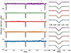 |
Fig. 1. ULTRACAM us, gs, rs, is, and SOAR phased-folded light curves (coloured points) of J2102−4145 with the best-fit light curve model over-plotted in black (left panel). Zoomed-in primary and secondary eclipses are also shown in the bottom-right and top-right panels, respectively. |
We started with a fixed 50% contribution from each star and changed the flux contribution according to the relative luminosities of the stars. For an ideal solution, the two threads must converge the same results within their respective error bars.
Once the spectral analysis converges and the relative changes of all stellar and binary parameters decrease below 0.5%, XTGRID calculates the errors by changing each parameter in one dimension until the chi-square change corresponds to the 60% confidence limit. Figure 2 shows the best-fit composite model for a representative VLT/X-shooter spectrum at orbital phase ϕ = 0.25. The inset plot in Fig. 2 depicts the RV differences for the primary and secondary components, revealing the binary nature. The same plot, but for the Gemini-GMOS data, can be seen in Fig. A.1.
The best fits for all X-shooter spectra can be seen in Fig. 3. The same plot, but for GMOS data, is shown in Fig. A.2. The Hα and Hβ composite line profiles are shown in the left and right panels, respectively, and are organised by the orbital phase. The final surface parameters and their errors are listed in Table 2.
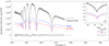 |
Fig. 2. Best-fit XTGRID with WD model to the VLT/X-shooter spectrum of J2102−4145 at orbital phase ϕ = 0.25 (maximum radial velocity difference) in the rest frame of the secondary. The observed spectrum can be reproduced by two nearly identical WD components (red and blue lines). At ϕ = 0.25 and 0.75, the components show the largest radial velocity difference and the double absorption core of the Hα reveals the binarity (inset). The phase-resolved spectral coverage for the entire orbit is available in Fig. 3. |
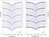 |
Fig. 3. Best-fit XTGRID with WD models and the spectral evolution of the composite Hα (right panel) and Hβ (left panel) composite line profiles in the VLT/X-shooter observations. Observations are in grey and black, where the black colour distinguishes orbital phases nearest to the conjunctions and quadratures. The composite model is in blue. We show here the continuum normalised spectra for easier stacking. All fits have been done on the original flux-calibrated data. |
Atmospheric parameters from the X-shooter spectra.
3.2. PHOEBE: Light curve fitting method
Since it has the highest signal-to-noise ratio of our full span of photometric data sets and consists of fast-cadence observations, we modelled the ULTRACAM light curves using the PHysics Of Eclipsing BinariEs v2.4 (PHOEBE, Prša et al. 2016; Horvat et al. 2018; Jones et al. 2020; Conroy et al. 2020) package to constrain all components of the binary. In addition, we simultaneously modelled the multi-band photometry and the primary and secondary RVs.
We assign both stars to have blackbody atmospheres and allow the secondary albedo to vary in each passband. Interpolated limb darkening coefficients following a power law were assigned to each star from the 3D WD models of Claret et al. (2020a). Interpolated gravity darkening coefficients were assigned using the tables of Claret et al. (2020b). The PHOEBE 2.2 Doppler beaming function was reinstated for our study (see Munday et al. 2023) and interpolated Doppler beaming coefficients from Claret et al. (2020a) were passed. For all of these interpolated components, the coefficients are unique for each of the Super SDSS filters and the respective tables were used for filters us, gs, rs, and is. The impact of smearing across a finite exposure time was corrected for assuming 9 s, 3 s, 3 s, and 3 s for the us, gs, rs, and is, respectively. Light-travel-time effects were handled with the PHOEBE code, accounting for Røemer delay. The synthetic RVs incorporate the impact of the stars’ surface gravity on the measured RVs and are determined from the centre of light of the system at a given phase.
In search for a system solution, we implemented an MCMC algorithm using the Python package EMCEE (Foreman-Mackey et al. 2013), where a series of walkers converged through minimisation of the χ2 between the observed light curves and the synthetic (and scaled) model light curves. The post burn-in posterior distribution of the MCMC was analysed using the CORNER python package (Foreman-Mackey 2016) and the resultant plot can be seen in Fig. C.1. The free parameters that we employed were combinations of the effective temperature (Teff), the radii and the masses of both stars, the secondary albedo in each passband, the systemic velocity and the system inclination.
The primary albedo was fixed at 1.0 in all bands as allowing both the primary and secondary to vary would lead to degeneracy between parameters and perhaps a nonphysical local minimum. There is also degeneracy between the star temperatures and the secondary albedo. To alleviate this, we first modelled with a fixed primary temperature as obtained from spectroscopy (see Table 2) and found secondary albedos of 1.04 ± 0.03, 1.01 ± 0.02, 1.00 ± 0.02, and 1.03 ± 0.05, for us, gs, rs, and is filters, respectively. To obtain a final model, we allowed the primary effective temperature to vary freely and forced Gaussian priors with the aforementioned secondary albedos. In this setup, the primary temperature is largely constrained by the interpolation of limb/gravity darkening models and its effect on the light curve morphology, while the secondary temperature is largely dependent on these same parameters and the relative eclipse depth. Furthermore, the eccentricity of the orbit was found to be very low, with an upper bound of e < 5 × 10⁻⁵ (2σ) or 2 × 10⁻⁵ (1σ), suggesting a nearly circular orbit.
Our resultant best-fit parameters are given in Table 3. In addition, the ULTRACAM us, gs, rs, is, and SOAR phase-folded light curves are shown in Fig. 1 with the best-fit for each light curve shown as a black line. We also depict the primary and secondary eclipses zoomed-in in the same figure. It is important to note that the SOAR and SMARTS-1m light curve were not used for this fit due to its lower cadence (∼30 s), resulting in a limited number of data points during each eclipse also a high smearing effect.
J2102−4145 system parameters from light curve fitting to the ULTRACAM photometry.
3.3. Light curve analysis: Looking for periodicities
To look for periodicities in the light curves due to pulsations, we used two different methods in order to remove the eclipses. The first consisted of solely masking the eclipses given that the duration of each eclipse is only 2 min. The second was subtracting the binary models from PHOEBE, and then using the residual light curve. In both cases, after each process, we calculated the Fourier Transform (FT), using the software Period04 (Lenz & Breger 2004). We accepted a frequency peak as significant if its amplitude exceeds an adopted significance threshold. In this work, the detection limit (dashed line in Figs. B.2–B.4) corresponds to the 1/1000 False Alarm Probability (FAP), where any peak with amplitude above this value has 0.1% probability of being a false detection due to noise. The FAP is calculated by shuffling the fluxes in the light curve while keeping the same time sampling, and computing the FT of the randomised data. This procedure is repeated N/2 times, where N is the number of points in the light curve. For each run, we compute the maximum amplitude of the FT. From the distribution of maxima, we take the 0.999 percentile as the detection limit (Romero et al. 2020). The internal uncertainties in frequency and amplitude were computed using a Monte Carlo method with 100 simulations with PERIOD04, while uncertainties in the periods were obtained through error propagation.
To ensure that the observed signal in our masked method is not influenced by the Doppler beaming effect, we generated a new PHOEBE model for SOAR and ULTRACAM data in us, gs, is, and rs bands removing the Doppler effect contribution. We thus subtract this new binary model from PHOEBE and subsequently analyse the residual light curve. This approach mirrors our previous methodology. This adjustment aimed to investigate and eliminate the possibility that the signals observed with masked eclipses (see Fig. B.2) were not caused by the Doppler beaming effect.
From the masking method, we found significant peaks in most of our data sets (see Fig. B.2). Yet, the same peaks were not seen in the FT for the residual light curves obtained by subtracting the binary model. This held true for both cases, whether the Doppler beaming effect was taken into account during the PHOEBE model calculation (Fig. B.3) or was not considered (Fig. B.4).
4. Results and discussion
J2102−4145 is an eclipsing double-lined and double-degenerate WD binary, as confirmed by Kosakowski et al. (2023). This star has a magnitude of G = 15.7 and is located at a Gaia-derived distance of 163.4 ± 1 pc (Bailer-Jones et al. 2021). Our investigation encompassed an extensive observational campaign, resulting in the acquisition of approximately 28 h of high-speed photometric data across multiple nights conducted using three different telescopes. These observations have provided critical insights into the orbital characteristics of this system, including parameters such as inclination and the orbital period, which was previously known from Kosakowski et al. (2023). Notably, our study yields highly precise parameter measurements, with a particular focus on the masses. Furthermore, these observations allowed us to determine the radii of both stellar components while simultaneously constraining the mass of each star.
Although Kosakowski et al. (2023) provided a comprehensive spectral analysis of this system, in this study we present an additional spectral analysis, by using our time-series spectroscopy data acquired independently with two different telescopes Gemini South/GMOS and VLT/X-shooter. This supplementary spectral analysis not only enhances the accuracy of the derived system’s fundamental properties but also enriches our understanding through comparative analysis.
4.1. The masses, radii, and effective temperatures of both WDs
We applied the iterative fitting procedure to disentangle the binary components from the Gemini/GMOS and X-shooter spectra, in conjunction with the model of the multi-band photometry ULTRACAM light curves. We determined the Teff and log g for both stars, which yielded the following parameters:  K, log g1 = 7.36 ± 0.01 for the primary star, and
  K, log g2 = 7.32 ± 0.01 for the secondary star. As well as the masses M1 = 0.375 ± 0.003 M⊙ for the primary star and M2 = 0.314 ± 0.003 M⊙ for the secondary star. Our mass estimates and Teff values are consistent with previous measurements, such as those reported by Kosakowski et al. (2023). Furthermore, our light curve fitting method enabled us to measure the radii of each individual WD. We obtained the following radii: R1 = 0.0211 ± 0.0002 R⊙ and
  . Additionally, we derived RVs from the X-shooter spectrum using only VIS arm data set. Those results can be seen in Fig. 4 and Table D.1, where the RV values for the primary star (RV1) are depicted as blue circles and red triangles for the secondary (RV2). We also show their respective sinusoidal fit, which yields to semi-amplitude values of K1 = 220.8 ± 0.7 km s−1 and K2 = 184.6 ± 0.8 km s−1. Our RV semi-amplitude values are comparable with the ones found by Kosakowski et al. (2023). The bottom plot of Fig. 4 shows the residuals for each RV curve. Those results are also consistent with previous measurements done by Kosakowski et al. (2023).
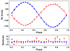 |
Fig. 4. Orbital solutions for each component of the double-lined binary J2102−4145 using X-shooter VIS arm data. The blue circle points represent the RV for the primary (hottest and more massive) star, while the red triangles represent the RVs for the secondary (cooler) star. |
A notable discrepancy is observed between the temperature and radius of the less massive WD, which appeared to be too hot for its derived mass and radius. This can be seen once we analysed the radius–Teff diagram in Fig. 5 in which the more massive star falls within the evolutionary models for the same derived mass, within its uncertainties. However, the less massive star should be much colder to match the models with a similar mass.
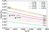 |
Fig. 5. Stellar radius as a function of the effective temperature for He-core WD evolutionary sequences with stellar masses going from 0.317 to 0.393 M⊙. The solid lines represent evolutionary models from Istrate et al. (2016) for metallicity of Z = 0.02, dotted lines are Istrate et al. (2016) models for metallicity Z = 0.001 and the dashed lines are models from Althaus et al. (2013) for metallicity Z = 0.001. Both stars of the eclipsing system J2102−4145, are shown in black circles, with their respective radius and Teff values found in this work. |
A possible explanation for this case includes heating during a CE phase or post-CE phase evolution (see Sect. 4.3 for further explanation). These processes may have influenced the secondary WD’s properties.
4.2. Periodicity in the light curve
As outlined in Sect. 3.3, two methods were employed to investigate potential periodicities in the residual light curve that could be indicative of pulsations. Initially, we applied a masking approach exclusively to the eclipses, revealing a distinct periodic variation primarily observed in the SOAR, ULTRACAM gs, and is bands. The corresponding FT results are presented in the top three panels of Fig. B.2, indicating a peak at a frequency of approximately ∼197.324594 μHz (equivalent to a period of 1.41 h). However, this periodicity was not consistently detected in other datasets, such as ULTRACAM us and rs, possibly due to higher cadence or increased noise levels.
Upon subtracting the binary model generated using PHOEBE, the same periodicity was not evident in the residual light curve in both cases, whether the Doppler beaming effect was taken into account during the PHOEBE model calculation (Fig. B.3) or was not considered (Fig. B.4). Nevertheless, this inconsistency raises doubts about the cause of this period.
However, it is worthwhile to note that the values derived in this study for effective temperature and log g placed both the primary and secondary stars outside the ZZ Ceti instability strip, as indicated by the green circles in Fig. 6. These findings align with the results presented in Kosakowski et al. (2023; illustrated by purple triangles in Fig. 6) for this same system.
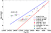 |
Fig. 6. Positions of the primary and the secondary stars of the binary system presented in this work, in the Teff − log g plane, are presented as green circles. The values of Teff and log g found in Kosakowski et al. (2023) for the same system are depicted as purple triangles. The other two pulsating WD in an eclipsing system found by Brown et al. (2023) are depicted as orange pentagons. The system found by Pyrzas et al. (2015) is depicted as a pink ×. The first confirmed pulsating WD in a double-degenerate eclipsing system from Parsons et al. (2020) is depicted as a blue square. The known ZZ Ceti (Romero et al. 2022) and ELMVs (Hermes et al. 2012, 2013a,b; Kilic et al. 2015; Bell et al. 2015, 2017; Pelisoli et al. 2018; Lopez et al. 2021) are shown as grey dots and black diamond shapes, respectively. The ELMV found by Guidry et al. (2021) is not being depicted since its atmospheric parameters have not been determined. The empirical ZZ Ceti instability strip published in Gianninas et al. (2015) is marked with dashed lines. |
In conclusion, the identified periodicity at a period of P = 1.41 h in specific light curves introduces intriguing possibilities but remains uncertain in its classification as a pulsation period and its verisimilitude. The potential impact of modelling artefacts and the contextual positioning of the system outside the ZZ Ceti instability strip underscores the need for a cautious interpretation of this observation.
4.3. Possible evolutionary path
Assuming that the primary (hottest) and most massive WD formed later implies that its progenitor was initially the less massive star in the system. This can be understood if we assume that the system underwent a first phase of mass transfer, which must have been stable, during which the progenitor of the low-mass WD lost its envelope while the mass of its main sequence (MS) companion increased. Given the current short orbital period (Porb = 2.4 h), the system must have later experienced a common envelope phase (CE, Paczynski 1976) when the progenitor of the hotter WD evolved towards the RGB.
In order to reconstruct the possible evolutionary history of this system, as well as its future, we used the Binary Star Evolution (BSE) code from Hurley et al. (2002). We started with initial binary systems composed of two MS stars and orbital periods below ∼3 days. The short orbital period ensures that the initially more massive star filled its Roche lobe before reaching the RGB phase, where the deep convective envelope would have most likely led to a CE phase. For the second mass transfer phase (the CE phase), BSE calculates the period after the CE is ejected using the standard α-formalism, that is,
 (2)
(2)
where Ebind is the binding energy of the envelope, ΔEorb is the change in orbital energy during the CE phase, and αCE is the CE efficiency, which corresponds to the fraction of ΔEorb that is used to unbind the envelope. The binding energy is calculated as:
 (3)
(3)
where Md, Md, e, and R are the total mass, envelope mass and radius of the donor at the onset of the CE phase. The binding energy parameter λ depends on the structure of the donor star, as well as on the inclusion or not of extra energy sources (in addition to gravitational and orbital) that might assist in unbinding the envelope. Some sources of additional energy suggested in the literature include thermal energy, hydrogen recombination energy, or enthalpy, but their contribution is still on debate (see Ivanova et al. 2013, for a comprehensive discussion). Nonetheless, any additional energy included would result in a reduced binding energy, that is, a larger value of λ.
The outcome of the CE phase is strongly dependent on the assumed values for αCE and λ. While αCE must be set as an input parameter in BSE, λ can either be set as a fixed value, or one can let the code calculate it. In the latter, one can also decide whether to include a fraction of the recombination energy. Given all the uncertainties in calculating λ, especially regarding what other potential sources of energy should be included, we have decided to set a fixed value of λ = 1. The CE efficiency αCE, on the other hand, was varied to ensure that the simulated systems survived the CE phase, resulting in very close but still detached binary systems.
We managed to reproduce systems similar to the one observed using initial masses in the range of ∼2 − 2.5 M⊙ for the primary and ≲1 M⊙ for its companion, with initial orbital periods in the range of ∼2−3 days, which caused the more massive star to fill its Roche lobe either towards the end of the MS or on the subgiant branch (Hertzsprung gap). An example of a possible evolutionary path obtained with the BSE code is shown in Fig. 7. The initial system in this sample is composed of two MS stars with masses of 2.30 M⊙ and 0.88 M⊙ at an orbital period of 2.2 days. The more massive star fills its Roche lobe on the Hertzsprung gap (HG). Initially, mass transfer from the more massive to the less massive star gradually decreases the orbital distance. However, when the donor star has transferred enough mass to its companion, the mass ratio reverses, and the orbital distance begins to increase. The donor star has time to reach the RGB phase, but as the orbital distance increases and the donor has a greatly reduced envelope, mass transfer remains stable. The mass transfer rate gradually decreases until the donor detaches from its Roche lobe and quickly becomes a low-mass helium WD, whose mass is not sufficient to ignite helium. The companion star, which accreted much of the mass transferred by the donor, becomes a blue straggler star (BSS), with a much larger mass than initially. This increase in mass accelerates its evolution and, since the orbital period is now longer than initially, it fills its Roche lobe when it is already on the RGB.
 |
Fig. 7. Example of a possible evolutionary path towards the observed system obtained with the BSE code from Hurley et al. (2002). The future of the system is also illustrated, based on the current masses and orbital period and assuming that angular momentum loss comes only from gravitational radiation. |
With a much larger mass ratio and the donor now in the RGB phase, this second mass transfer phase becomes dynamically unstable, triggering a CE phase. A very high CE efficiency (αCE > 5) was needed in order to survive the CE phase without merging. In the particular case we illustrated in Fig. 7 we used αCE = 6.6, in order to match the observed period at the predicted current time. This was based on the cooling age of the more massive WD in the observed system, which was estimated to be between ∼200 and ∼300 Myr based on the tracks for low-mass WDs from Althaus et al. (2013). For several of the configurations that resulted in simulated systems similar to the observed one, the core of the giant that expelled its envelope during the CE phase had enough mass to ignite helium, becoming a hot subdwarf star (sdB). For a mass of ∼0.37 M⊙, the stable core helium burning phase lasts about 500 million years (Arancibia-Rojas et al. 2024), until helium is depleted in the core. The star then goes through a brief sdO phase (a few million years, not shown in the figure) and ultimately becomes a WD, likely with a hybrid (He/CO) composition. The detached system is now composed of two low-mass WDs at a very short orbital period, which is decreasing due to gravitational radiation, until the two remnants merge to form a single WD. Given the observed orbital period and masses, this should occur in around 800 Myr (regardless of the previous evolution). The merger of the two low-mass WDs will trigger helium ignition, leading to the formation of a helium-rich hot subdwarf star undergoing core helium burning for ∼100 Myr, after which the object will evolve into a hybrid He/CO WD (see e.g. Zhang & Jeffery 2012; Dan et al. 2014; Schwab 2018). However, we decided not to include the mass of the resulting remnant in this figure, because the outcome of the merger also depends on how fast the merger process occurs (Zhang & Jeffery 2012).
We note that the example shown here is just an illustrative case of a possible evolutionary path given by the BSE code for a similar system, and we are not claiming that this was really the evolution experienced by J2102−4145. Here we discuss some uncertainties with respect to the evolution.
(1) The CE phase is poorly understood, and especially the efficiency parameter (αCE) and the structural parameter (λ) are not well constrained. A low efficiency (αCE ∼ 0.3) has been derived from the observed samples of close WDs with unevolved companions, including low-mass (spectral type M) MS companions (Zorotovic et al. 2010; Toonen & Nelemans 2013; Camacho et al. 2014), intermediate-mass (spectral type K to A) MS companions (Hernandez et al. 2022, and references therein), or brown dwarfs (Zorotovic & Schreiber 2022). For double WD systems, a larger efficiency (αCE ∼ 2, assuming λ = 1) was favoured by Nelemans et al. (2000), while recently Scherbak & Fuller (2023) also derived a low efficiency (αCE ∼ 1/3) when backtracking the second mass transfer phase in double degenerate systems with low-mass (helium-core) WDs. Reconstructing the evolution of J2102−4145 with BSE requires an unusually high efficiency (αCEλ > 5), which seems to be physically implausible. Nonetheless, a recent study by Renzo et al. (2023) demonstrated that rejuvenated stars, such as the proposed progenitor for the more massive WD in this system, possess significantly less bound envelopes. This implies that the binding energy parameter λ should be considerably larger than that of normal stars, resulting in a lower value for αCE, which might be consistent with αCE < 1. It is worth noting, however, that the calculations in Renzo et al. (2023) focused on massive rejuvenated stars, that will evolve into either a neutron star or a black hole. The authors suggest that a similar scenario may apply to lower-mass accretors, as far as they have a convective core on the MS (MZAMS ≳ 1.2 M⊙). In the example we present, the accretor has a smaller initial mass, so it likely had a radiative core and a convective envelope during the MS phase, before accreting the mass from its initially more massive companion. Consequently, the impact of accretion on the envelope’s binding energy remains uncertain in this specific case.
(2) Depending on the mass transfer rate, stable mass transfer can either be near fully conservative or highly non-conservative. By examining the total mass before and after the stable mass transfer phase in Fig. 7, we found that the first mass transfer phase was highly conservative, with a total mass loss from the system of approximately 6%. The BSE code does not provide the option to modify this conservativeness. However, a less conservative stable mass transfer phase would have resulted in a larger orbital separation at the end of mass transfer and a lower mass for the progenitor of the more massive WD. The increased orbital separation would have allowed the companion star to fill its Roche lobe later on the RGB, attaining a core mass similar to the observed one when its radius was larger. With a less massive and more extended envelope, the process of envelope ejection would have been facilitated, resulting in a reduced value of αCE.
(3) The core helium burning phase (as an sdB star) may or may not have occurred, depending on the mass that the progenitor of the secondly formed WD had before losing the envelope. For a core with less than 0.4 M⊙ to ignite helium after losing the envelope, the progenitor must have been more massive than ∼1.8 M⊙ (Han et al. 2002; Arancibia-Rojas et al. 2024). Less massive progenitors develop highly degenerate cores during the RGB phase and therefore require a higher core mass to trigger helium burning. Therefore, if the mass transfer was substantially less conservative than in our example, with more than ∼1 M⊙ lost from the system, a 0.37 M⊙ core would not have ignited helium and would have quickly become a helium WD after the CE phase. To test the effects of mass transfer conservativeness on the evolution, a more flexible and detailed stellar evolutionary code, such as MESA (Paxton et al. 2011), should be used. However, this goes beyond the scope of this work, as we are only presenting a possible evolutionary scenario. The occurrence of a hot subdwarf phase could provide an explanation for the high effective temperature of the less massive WD. As we saw in Sect. 4.1, the less massive WD in J2102−4145 has a very high effective temperature for the derived mass and radius. It is unlikely that the CE phase is responsible for the higher temperature, because this phase is too short and the accretor is not expected to retain any mass, and therefore any increase in effective temperature should rapidly diminish after the envelope ejection. The sdB phase, on the other hand, can last for approximately half a Gyr for a 0.37 M⊙ sdB, which could be sufficient to produce a long-lasting effect on the temperature of a close companion, especially if there was wind mass transfer from the hot subdwarf (more likely during the sdO phase) to the lower mass WD. If the core helium-burning phase is necessary, it implies that the assumption of highly conservative stable mass transfer is not too far from reproducing the actual evolutionary history of the system.
5. Summary
In this section, we present the key results and findings from our investigation of the eclipsing double-lined and double-degenerate WD binary system, J2102−4145. This system was previously confirmed in the study by Kosakowski et al. (2023), and our research builds upon and enhances our understanding of its properties.
Our study involved an extensive observational campaign, which spanned multiple nights and included data collected from three different telescopes, NTT/ULTRACAM, SOAR/Goodman, and SMARTS-1m, in which we acquired approximately 28 hours of high-speed photometric data. Also, while Kosakowski et al. (2023) had performed a comprehensive spectral analysis of J2102−4145, our study contributed supplementary spectral analysis conducted independently with two different telescopes: Gemini South/GMOS and VLT/X-shooter.
Our observations provided crucial insights into the orbital characteristics of J2102−4145. This included the determination of parameters such as the orbital inclination of  deg and the orbital period of Porb = 2.4 h, in which the last had been previously known from the work of Kosakowski et al. (2023). A central focus of our study was to achieve highly precise parameter measurements for the J2102−4145, binary system. We placed particular emphasis on accurately determining the masses of both WDs within the binary, giving us the values of M1 = 0.375 ± 0.003 M⊙ for the primary and M2 = 0.314 ± 0.003 M⊙ for the secondary. In addition to mass measurements, our observations allowed us to determine the radii, Teff and log g of both WD components: R1 = 0.0211 ± 0.0002 R⊙,
  K and log g1 = 7.36 ± 0.01 dex for the primary and
  ,
,  K and log g2 = 7.32 ± 0.01 dex for the secondary. This radius information adds to the overall understanding of the system’s properties.
From the X-shooter spectrum, we obtained radial velocity measurements that included semi-amplitude values of K1 = 220.8 ± 0.7 km s−1 for the primary star and K2 = 184.6 ± 0.8 km s−1 for the secondary star. Similar values were also found by Kosakowski et al. (2023). The consistency between our results and those of previous studies significantly supports our confidence in the conclusions drawn from this analysis.
Also, our investigation into potential periodicities in the residual light curve, employing two methods, revealed a periodic variation of approximately 1.41 h in specific bands. However, the inconsistent detection of this periodicity across all datasets raises doubts about its classification as a pulsation. Additionally, our analysis placing both stars outside the ZZ Ceti instability strip aligns with previous findings. The cause of the identified periodicity, while intriguing, remains uncertain in its nature and authenticity as a pulsation period. Considering the potential impact of modelling artefacts and the system’s contextual position outside the ZZ Ceti instability strip, caution is warranted in interpreting this observation.
An intriguing finding was the temperature and radius discrepancy observed in the less massive WD. The secondary star appeared hotter than expected for its mass and radius, prompting discussions about possible explanations, such as heating during a CE phase or post-CE phase evolution. We discussed a possible evolutionary path for the J2102−4145, system, which included initial mass transfer, a CE phase, and the eventual formation of two low-mass WD. While this serves as an illustrative example, it highlights the complexity of the system’s evolutionary history. Acknowledging uncertainties, particularly concerning the CE phase and mass transfer conservativeness, we considered the occurrence of a hot subdwarf phase as a potential explanation for the high Teff of the less massive WD.
In conclusion, our study contributes valuable insights into the J2102−4145, system, shedding light on its fundamental properties and potential evolutionary history. These findings enrich our understanding of binary WD systems and the intricate pathways they traverse.
Acknowledgments
We thank the anonymous referee for their suggestions, which helped improve our manuscript. L.A.A. acknowledges financial support from CONICYT Doctorado Nacional in the form of grant number No: 21201762 and ESO studentship programme. Based on observations collected with the GMOS spectrograph on the 8.1 m Gemini-South telescope at Cerro Pachón, Chile, under the programme GS-2022A-Q-416, and observation with Goodman SOAR 4.1 m telescope, at Cerro Pachón, Chile, and SMARTS-1m telescope at Cerro Tololo, Chile, under the programme allocated by the Chilean Time Allocation Committee (CNTAC), no: CN2022A-412490, and SOAR observational time through NOAO programme SO2021A-008_0516. J.M. was supported by funding from a Science and Technology Facilities Council (STFC) studentship. ULTRACAM operations and VSD are funded by the Science and Technology Facilities Council (grant ST/V000853/1). M.V. acknowledges support from FONDECYT (grant No: 1211941). I.P. acknowledges a Warwick Astrophysics prize post-doctoral fellowship made possible thanks to a generous philanthropic donation. P.N. acknowledges support from the Grant Agency of the Czech Republic (GAČR 22-34467S). The Astronomical Institute in Ondřejov is supported by the project RVO:67985815. This research has used the services of www.Astroserver.org under reference XG61YQ.
References
- Althaus, L. G., Miller Bertolami, M. M., & Córsico, A. H. 2013, A&A, 557, A19 [NASA ADS] [CrossRef] [EDP Sciences] [Google Scholar]
- Amaro-Seoane, P., Audley, H., Babak, S., et al. 2017, arXiv e-prints [arXiv:1702.00786] [Google Scholar]
- Arancibia-Rojas, E., Zorotovic, M., Vučković, M., et al. 2024, MNRAS, 527, 11184 [Google Scholar]
- Bailer-Jones, C. A. L., Rybizki, J., Fouesneau, M., Demleitner, M., & Andrae, R. 2021, AJ, 161, 147 [Google Scholar]
- Bell, K. J., Kepler, S. O., Montgomery, M. H., et al. 2015, in 19th European Workshop on White Dwarfs, eds. P. Dufour, P. Bergeron, & G. Fontaine, ASP Conf. Ser., 493, 217 [Google Scholar]
- Bell, K. J., Gianninas, A., Hermes, J. J., et al. 2017, ApJ, 835, 180 [Google Scholar]
- Bildsten, L., Shen, K. J., Weinberg, N. N., & Nelemans, G. 2007, ApJ, 662, L95 [Google Scholar]
- Brown, W. R., Kilic, M., Allende Prieto, C., & Kenyon, S. J. 2010, ApJ, 723, 1072 [Google Scholar]
- Brown, W. R., Gianninas, A., Kilic, M., Kenyon, S. J., & Allende Prieto, C. 2016, ApJ, 818, 155 [Google Scholar]
- Brown, W. R., Kilic, M., Kosakowski, A., & Gianninas, A. 2022, ApJ, 933, 94 [NASA ADS] [CrossRef] [Google Scholar]
- Brown, A. J., Parsons, S. G., van Roestel, J., et al. 2023, MNRAS, 521, 1880 [NASA ADS] [CrossRef] [Google Scholar]
- Camacho, J., Torres, S., García-Berro, E., et al. 2014, A&A, 566, A86 [NASA ADS] [CrossRef] [EDP Sciences] [Google Scholar]
- Claret, A., Cukanovaite, E., Burdge, K., et al. 2020a, A&A, 641, A157 [NASA ADS] [CrossRef] [EDP Sciences] [Google Scholar]
- Claret, A., Cukanovaite, E., Burdge, K., et al. 2020b, A&A, 634, A93 [EDP Sciences] [Google Scholar]
- Conroy, K. E., Kochoska, A., Hey, D., et al. 2020, ApJS, 250, 34 [Google Scholar]
- Dan, M., Rosswog, S., Brüggen, M., & Podsiadlowski, P. 2014, MNRAS, 438, 14 [NASA ADS] [CrossRef] [Google Scholar]
- Dhillon, V. S., Marsh, T. R., Stevenson, M. J., et al. 2007, MNRAS, 378, 825 [NASA ADS] [CrossRef] [Google Scholar]
- Dhillon, V. S., Bezawada, N., Black, M., et al. 2021, MNRAS, 507, 350 [NASA ADS] [CrossRef] [Google Scholar]
- Foreman-Mackey, D. 2016, J. Open Source Softw., 1, 24 [Google Scholar]
- Foreman-Mackey, D., Hogg, D. W., Lang, D., & Goodman, J. 2013, PASP, 125, 306 [Google Scholar]
- Gianninas, A., Kilic, M., Brown, W. R., Canton, P., & Kenyon, S. J. 2015, ApJ, 812, 167 [Google Scholar]
- Gimeno, G., Roth, K., Chiboucas, K., et al. 2016, in Ground-based and Airborne Instrumentation for Astronomy VI, eds. C. J. Evans, L. Simard, & H. Takami, SPIE Conf. Ser., 9908, 99082S [NASA ADS] [Google Scholar]
- Guidry, J. A., Vanderbosch, Z. P., Hermes, J. J., et al. 2021, ApJ, 912, 125 [NASA ADS] [CrossRef] [Google Scholar]
- Han, Z., Tout, C. A., & Eggleton, P. P. 2000, MNRAS, 319, 215 [Google Scholar]
- Han, Z., Podsiadlowski, P., Maxted, P. F. L., Marsh, T. R., & Ivanova, N. 2002, MNRAS, 336, 449 [Google Scholar]
- Hermes, J. J., Montgomery, M. H., Winget, D. E., et al. 2012, ApJ, 750, L28 [Google Scholar]
- Hermes, J. J., Montgomery, M. H., Winget, D. E., et al. 2013a, in 18th European White Dwarf Workshop, eds. J. Krzesiński, G. Stachowski, P. Moskalik, & K. Bajan, ASP Conf. Ser., 469, 57 [Google Scholar]
- Hermes, J. J., Montgomery, M. H., Gianninas, A., et al. 2013b, MNRAS, 436, 3573 [Google Scholar]
- Hermes, J. J., Brown, W. R., Kilic, M., et al. 2014, ApJ, 792, 39 [NASA ADS] [CrossRef] [Google Scholar]
- Hernandez, M. S., Schreiber, M. R., Parsons, S. G., et al. 2022, MNRAS, 517, 2867 [NASA ADS] [CrossRef] [Google Scholar]
- Hook, I. M., Jørgensen, I., Allington-Smith, J. R., et al. 2004, PASP, 116, 425 [NASA ADS] [CrossRef] [Google Scholar]
- Horvat, M., Conroy, K. E., Pablo, H., et al. 2018, ApJS, 237, 26 [Google Scholar]
- Hurley, J. R., Tout, C. A., & Pols, O. R. 2002, MNRAS, 329, 897 [Google Scholar]
- Iben, I., Jr., & Livio, M. 1993, PASP, 105, 1373 [CrossRef] [Google Scholar]
- Iben, I., Jr., & Tutukov, A. V. 1984, ApJS, 54, 335 [NASA ADS] [CrossRef] [Google Scholar]
- Iben, I., Jr., & Tutukov, A. V. 1985, ApJS, 58, 661 [NASA ADS] [CrossRef] [Google Scholar]
- Iben, I., Jr., & Tutukov, A. V. 1986, ApJ, 311, 753 [NASA ADS] [CrossRef] [Google Scholar]
- Istrate, A. G., Tauris, T. M., & Langer, N. 2014, A&A, 571, A45 [NASA ADS] [CrossRef] [EDP Sciences] [Google Scholar]
- Istrate, A. G., Marchant, P., Tauris, T. M., et al. 2016, A&A, 595, A35 [NASA ADS] [CrossRef] [EDP Sciences] [Google Scholar]
- Ivanova, N., Justham, S., Chen, X., et al. 2013, A&ARv, 21, 59 [Google Scholar]
- Jones, D., Conroy, K. E., Horvat, M., et al. 2020, ApJS, 247, 63 [Google Scholar]
- Kepler, S. O., Koester, D., Romero, A. D., Ourique, G., & Pelisoli, I. 2017, in 20th European White Dwarf Workshop, eds. P. E. Tremblay, B. Gaensicke, & T. Marsh, ASP Conf. Ser., 509, 421 [Google Scholar]
- Kilic, M., Hermes, J. J., Gianninas, A., & Brown, W. R. 2015, MNRAS, 446, L26 [Google Scholar]
- Kilic, M., Bergeron, P., Kosakowski, A., et al. 2020, ApJ, 898, 84 [Google Scholar]
- Kilic, M., Bergeron, P., Blouin, S., & Bédard, A. 2021, MNRAS, 503, 5397 [NASA ADS] [CrossRef] [Google Scholar]
- Kosakowski, A., Brown, W. R., Kilic, M., et al. 2023, ApJ, 950, 141 [CrossRef] [Google Scholar]
- Lauffer, G. R., Romero, A. D., & Kepler, S. O. 2018, MNRAS, 480, 1547 [NASA ADS] [CrossRef] [Google Scholar]
- Lenz, P., & Breger, M. 2004, in The A-Star Puzzle, eds. J. Zverko, J. Ziznovsky, S. J. Adelman, & W. W. Weiss, 224, 786 [Google Scholar]
- Li, Z., Chen, X., Chen, H.-L., & Han, Z. 2019, ApJ, 871, 148 [NASA ADS] [CrossRef] [Google Scholar]
- Liebert, J., Bergeron, P., Eisenstein, D., et al. 2004, ApJ, 606, L147 [NASA ADS] [CrossRef] [Google Scholar]
- Lopez, I. D., Hermes, J. J., Calcaferro, L. M., et al. 2021, ApJ, 922, 220 [NASA ADS] [CrossRef] [Google Scholar]
- Marsh, T. R., Dhillon, V. S., & Duck, S. R. 1995, MNRAS, 275, 828 [Google Scholar]
- Munday, J., Tremblay, P. E., Hermes, J. J., et al. 2023, MNRAS, 525, 1814 [NASA ADS] [CrossRef] [Google Scholar]
- Nelemans, G., Verbunt, F., Yungelson, L. R., & Portegies Zwart, S. F. 2000, A&A, 360, 1011 [NASA ADS] [Google Scholar]
- Németh, P., Kawka, A., & Vennes, S. 2012, MNRAS, 427, 2180 [Google Scholar]
- Paczynski, B. 1976, in Structure and Evolution of Close Binary Systems, eds. P. Eggleton, S. Mitton, & J. Whelan, 73, 75 [NASA ADS] [CrossRef] [Google Scholar]
- Panei, J. A., Althaus, L. G., Chen, X., & Han, Z. 2007, MNRAS, 382, 779 [Google Scholar]
- Parsons, S. G., Brown, A. J., Littlefair, S. P., et al. 2020, Nat. Astron., 4, 690 [Google Scholar]
- Paxton, B., Bildsten, L., Dotter, A., et al. 2011, ApJS, 192, 3 [Google Scholar]
- Pelisoli, I., & Vos, J. 2019, MNRAS, 488, 2892 [Google Scholar]
- Pelisoli, I., Kepler, S. O., Koester, D., et al. 2018, MNRAS, 478, 867 [Google Scholar]
- Prada Moroni, P. G., & Straniero, O. 2009, A&A, 507, 1575 [NASA ADS] [CrossRef] [EDP Sciences] [Google Scholar]
- Prša, A., Conroy, K. E., Horvat, M., et al. 2016, ApJS, 227, 29 [Google Scholar]
- Pyrzas, S., Gänsicke, B. T., Hermes, J. J., et al. 2015, MNRAS, 447, 691 [Google Scholar]
- Renzo, M., Zapartas, E., Justham, S., et al. 2023, ApJ, 942, L32 [NASA ADS] [CrossRef] [Google Scholar]
- Romero, A. D., Antunes Amaral, L., Kepler, S. O., et al. 2020, MNRAS, 497, L24 [Google Scholar]
- Romero, A. D., Kepler, S. O., Hermes, J. J., et al. 2022, MNRAS, 511, 1574 [NASA ADS] [CrossRef] [Google Scholar]
- Scherbak, P., & Fuller, J. 2023, MNRAS, 518, 3966 [Google Scholar]
- Schwab, J. 2018, MNRAS, 476, 5303 [Google Scholar]
- Shporer, A., Kaplan, D. L., Steinfadt, J. D. R., et al. 2010, ApJ, 725, L200 [Google Scholar]
- Steinfadt, J. D. R., Bildsten, L., & Arras, P. 2010, ApJ, 718, 441 [Google Scholar]
- Toonen, S., & Nelemans, G. 2013, A&A, 557, A87 [NASA ADS] [CrossRef] [EDP Sciences] [Google Scholar]
- Tremblay, P. E., & Bergeron, P. 2009, ApJ, 696, 1755 [Google Scholar]
- Tremblay, P. E., Ludwig, H. G., Steffen, M., & Freytag, B. 2013, A&A, 559, A104 [NASA ADS] [CrossRef] [EDP Sciences] [Google Scholar]
- Tremblay, P. E., Fontaine, G., Freytag, B., et al. 2015, ApJ, 812, 19 [Google Scholar]
- Tremblay, P. E., Cummings, J., Kalirai, J. S., et al. 2016, MNRAS, 461, 2100 [NASA ADS] [CrossRef] [Google Scholar]
- Tremblay, P. E., Hollands, M. A., Gentile Fusillo, N. P., et al. 2020, MNRAS, 497, 130 [NASA ADS] [CrossRef] [Google Scholar]
- Vernet, J., Dekker, H., D’Odorico, S., et al. 2011, A&A, 536, A105 [NASA ADS] [CrossRef] [EDP Sciences] [Google Scholar]
- Wang, K., Németh, P., Luo, Y., et al. 2022, ApJ, 936, 5 [CrossRef] [Google Scholar]
- Webbink, R. F. 1984, ApJ, 277, 355 [NASA ADS] [CrossRef] [Google Scholar]
- Zenati, Y., Toonen, S., & Perets, H. B. 2019, MNRAS, 482, 1135 [NASA ADS] [CrossRef] [Google Scholar]
- Zhang, X., & Jeffery, C. S. 2012, MNRAS, 419, 452 [NASA ADS] [CrossRef] [Google Scholar]
- Zorotovic, M., & Schreiber, M. R. 2017, MNRAS, 466, L63 [CrossRef] [Google Scholar]
- Zorotovic, M., & Schreiber, M. 2022, MNRAS, 513, 3587 [NASA ADS] [CrossRef] [Google Scholar]
- Zorotovic, M., Schreiber, M. R., Gänsicke, B. T., & Nebot Gómez-Morán, A. 2010, A&A, 520, A86 [NASA ADS] [CrossRef] [EDP Sciences] [Google Scholar]
Appendix A: Extra GMOS/Gemini-South spectra
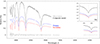 |
Fig. A.1. Best-fit XTGRID with WD model to the Gemini/GMOS spectrum of J2102-4145 at orbital phase ϕ = 0.75 (maximum radial velocity difference) in the rest frame of the secondary. The observed spectrum can be reproduced by two nearly identical WD components (red and blue lines). The phase-resolved spectral coverage for the entire orbit is available in Figure A.2. The wavelength gap between ∼520–625 nm is due to the bad amplifier number 5 (see Section 2.2). The flux of the observation was adjusted to the flux level of the theoretical composite continuum. |
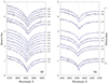 |
Fig. A.2. Best-fit XTGRID with WD models and the spectral evolution of the composite Hα (right panel) and Hβ (left panel) composite line profiles in the Gemini/GMOS observations in the rest frame of the primary. The fluxes of the observations were adjusted to the flux level of the theoretical composite continuum. |
Appendix B: Light curve analysis for periodicity
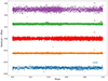 |
Fig. B.1. ULTRACAM light curve residuals after subtraction of the binary model in us, gs, rs, is, and SOAR, respectively. |
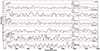 |
Fig. B.2. FT for J2102-4145, for SOAR, ULTRACAM us, gs, is, rs, and SMARTS-1m observations. The 1/1000 FAP detection limit (red dashed line) was computed using random shuffling of the data. The spectral window for each case is depicted as an inset plot, with the x-axis in μHz and all inset plots being in the same scale. For the rs ULTRACAM data, the combination (f1 + f2)/2 of the periods of 1.61 h (171.872 μHz) and 1.01 hr (274.345 μHz) its half of the orbital period. |
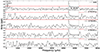 |
Fig. B.3. FT for J2102-4145, for SOAR, ULTRACAM us, gs, is, and rs for the residual light curve subsequent to subtracting the light curve fit generated using PHOEBE (see Section 3.3 for further information). The 1/1000 FAP detection limit (red dashed line) was computed using random shuffling of the data. The spectral window for each case is depicted as an inset plot, with the x-axis in μHz and all inset plots being in the same scale. For the SOAR data, although the 6.17 hr is above our threshold, it exceeds the duration of our light curve, which makes it less reliable. |
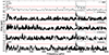 |
Fig. B.4. For the target J2102-4145 observed with SOAR and ULTRACAM us, gs, is, and rs FT analysis on the residual light curve, obtained after subtracting the light curve fit generated using PHOEBE (details in Section 3.3). The SOAR and ULTRACAM data in us, gs, is, and rs bands were used, mirroring the approach undertaken for Figure B.3. However, in this case, a new PHOEBE model was applied without considering the Doppler beaming effect. This adjustment aimed to investigate and eliminate the possibility that the 1.4-hour signal observed with masked eclipses (see Figure B.2) was caused by the Doppler beaming effect. |
Appendix C: Posterior probability distributions
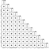 |
Fig. C.1. Corner plot of the phoebe2 MCMC (Foreman-Mackey 2016) posteriors for the primary mass (M1) and radius (R1), the secondary mass (M2), radius (R2) and effective temperature (T2), as well as the binary orbital inclination (i). |
Appendix D: Extra tables
RV values for the primary and secondary star.
Primary and secondary eclipse timings for the J2102-4145 system.
All Tables
J2102−4145 system parameters from light curve fitting to the ULTRACAM photometry.
All Figures
|
Fig. 1. ULTRACAM us, gs, rs, is, and SOAR phased-folded light curves (coloured points) of J2102−4145 with the best-fit light curve model over-plotted in black (left panel). Zoomed-in primary and secondary eclipses are also shown in the bottom-right and top-right panels, respectively. |
| In the text | |
|
Fig. 2. Best-fit XTGRID with WD model to the VLT/X-shooter spectrum of J2102−4145 at orbital phase ϕ = 0.25 (maximum radial velocity difference) in the rest frame of the secondary. The observed spectrum can be reproduced by two nearly identical WD components (red and blue lines). At ϕ = 0.25 and 0.75, the components show the largest radial velocity difference and the double absorption core of the Hα reveals the binarity (inset). The phase-resolved spectral coverage for the entire orbit is available in Fig. 3. |
| In the text | |
|
Fig. 3. Best-fit XTGRID with WD models and the spectral evolution of the composite Hα (right panel) and Hβ (left panel) composite line profiles in the VLT/X-shooter observations. Observations are in grey and black, where the black colour distinguishes orbital phases nearest to the conjunctions and quadratures. The composite model is in blue. We show here the continuum normalised spectra for easier stacking. All fits have been done on the original flux-calibrated data. |
| In the text | |
|
Fig. 4. Orbital solutions for each component of the double-lined binary J2102−4145 using X-shooter VIS arm data. The blue circle points represent the RV for the primary (hottest and more massive) star, while the red triangles represent the RVs for the secondary (cooler) star. |
| In the text | |
|
Fig. 5. Stellar radius as a function of the effective temperature for He-core WD evolutionary sequences with stellar masses going from 0.317 to 0.393 M⊙. The solid lines represent evolutionary models from Istrate et al. (2016) for metallicity of Z = 0.02, dotted lines are Istrate et al. (2016) models for metallicity Z = 0.001 and the dashed lines are models from Althaus et al. (2013) for metallicity Z = 0.001. Both stars of the eclipsing system J2102−4145, are shown in black circles, with their respective radius and Teff values found in this work. |
| In the text | |
|
Fig. 6. Positions of the primary and the secondary stars of the binary system presented in this work, in the Teff − log g plane, are presented as green circles. The values of Teff and log g found in Kosakowski et al. (2023) for the same system are depicted as purple triangles. The other two pulsating WD in an eclipsing system found by Brown et al. (2023) are depicted as orange pentagons. The system found by Pyrzas et al. (2015) is depicted as a pink ×. The first confirmed pulsating WD in a double-degenerate eclipsing system from Parsons et al. (2020) is depicted as a blue square. The known ZZ Ceti (Romero et al. 2022) and ELMVs (Hermes et al. 2012, 2013a,b; Kilic et al. 2015; Bell et al. 2015, 2017; Pelisoli et al. 2018; Lopez et al. 2021) are shown as grey dots and black diamond shapes, respectively. The ELMV found by Guidry et al. (2021) is not being depicted since its atmospheric parameters have not been determined. The empirical ZZ Ceti instability strip published in Gianninas et al. (2015) is marked with dashed lines. |
| In the text | |
|
Fig. 7. Example of a possible evolutionary path towards the observed system obtained with the BSE code from Hurley et al. (2002). The future of the system is also illustrated, based on the current masses and orbital period and assuming that angular momentum loss comes only from gravitational radiation. |
| In the text | |
|
Fig. A.1. Best-fit XTGRID with WD model to the Gemini/GMOS spectrum of J2102-4145 at orbital phase ϕ = 0.75 (maximum radial velocity difference) in the rest frame of the secondary. The observed spectrum can be reproduced by two nearly identical WD components (red and blue lines). The phase-resolved spectral coverage for the entire orbit is available in Figure A.2. The wavelength gap between ∼520–625 nm is due to the bad amplifier number 5 (see Section 2.2). The flux of the observation was adjusted to the flux level of the theoretical composite continuum. |
| In the text | |
|
Fig. A.2. Best-fit XTGRID with WD models and the spectral evolution of the composite Hα (right panel) and Hβ (left panel) composite line profiles in the Gemini/GMOS observations in the rest frame of the primary. The fluxes of the observations were adjusted to the flux level of the theoretical composite continuum. |
| In the text | |
|
Fig. B.1. ULTRACAM light curve residuals after subtraction of the binary model in us, gs, rs, is, and SOAR, respectively. |
| In the text | |
|
Fig. B.2. FT for J2102-4145, for SOAR, ULTRACAM us, gs, is, rs, and SMARTS-1m observations. The 1/1000 FAP detection limit (red dashed line) was computed using random shuffling of the data. The spectral window for each case is depicted as an inset plot, with the x-axis in μHz and all inset plots being in the same scale. For the rs ULTRACAM data, the combination (f1 + f2)/2 of the periods of 1.61 h (171.872 μHz) and 1.01 hr (274.345 μHz) its half of the orbital period. |
| In the text | |
|
Fig. B.3. FT for J2102-4145, for SOAR, ULTRACAM us, gs, is, and rs for the residual light curve subsequent to subtracting the light curve fit generated using PHOEBE (see Section 3.3 for further information). The 1/1000 FAP detection limit (red dashed line) was computed using random shuffling of the data. The spectral window for each case is depicted as an inset plot, with the x-axis in μHz and all inset plots being in the same scale. For the SOAR data, although the 6.17 hr is above our threshold, it exceeds the duration of our light curve, which makes it less reliable. |
| In the text | |
|
Fig. B.4. For the target J2102-4145 observed with SOAR and ULTRACAM us, gs, is, and rs FT analysis on the residual light curve, obtained after subtracting the light curve fit generated using PHOEBE (details in Section 3.3). The SOAR and ULTRACAM data in us, gs, is, and rs bands were used, mirroring the approach undertaken for Figure B.3. However, in this case, a new PHOEBE model was applied without considering the Doppler beaming effect. This adjustment aimed to investigate and eliminate the possibility that the 1.4-hour signal observed with masked eclipses (see Figure B.2) was caused by the Doppler beaming effect. |
| In the text | |
|
Fig. C.1. Corner plot of the phoebe2 MCMC (Foreman-Mackey 2016) posteriors for the primary mass (M1) and radius (R1), the secondary mass (M2), radius (R2) and effective temperature (T2), as well as the binary orbital inclination (i). |
| In the text | |
Current usage metrics show cumulative count of Article Views (full-text article views including HTML views, PDF and ePub downloads, according to the available data) and Abstracts Views on Vision4Press platform.
Data correspond to usage on the plateform after 2015. The current usage metrics is available 48-96 hours after online publication and is updated daily on week days.
Initial download of the metrics may take a while.