| Issue |
A&A
Volume 694, February 2025
|
|
|---|---|---|
| Article Number | A243 | |
| Number of page(s) | 13 | |
| Section | Astronomical instrumentation | |
| DOI | https://doi.org/10.1051/0004-6361/202453051 | |
| Published online | 18 February 2025 | |
Tackling artefacts in the timing of relativistic pulsar binaries: Towards the SKA
1
Max-Planck-Institut für Radioastronomie,
Auf dem Hügel 69,
53121
Bonn,
Germany
2
Dipartimento di Fisica “G. Occhialini”, Università degli Studi di Milano-Bicocca,
Piazza della Scienza 3,
Milano
20126,
Italy
3
Manly Astrophysics,
15/41-42 East Esplanade,
Manly,
NSW 2095,
Australia
4
Jodrell Bank Centre for Astrophysics, Department of Physics and Astronomy, University of Manchester,
Manchester
M13 9PL,
UK
★ Corresponding author; This email address is being protected from spambots. You need JavaScript enabled to view it.
; This email address is being protected from spambots. You need JavaScript enabled to view it.
Received:
18
November
2024
Accepted:
26
January
2025
Abstract
Common signal-processing approximations produce artefacts when timing pulsars in relativistic binary systems, especially edge-on systems with tight orbits, such as the Double Pulsar. In this paper, we use extensive simulations to explore various patterns that arise from the inaccuracies of approximations made when correcting dispersion and Shapiro delay. In a relativistic binary, the velocity of the pulsar projected onto the line of sight varies significantly on short timescales, causing rapid changes in the apparent pulsar spin frequency, which is used to convert dispersive delays to pulsar rotational phase shifts. A well-known example of the consequences of this effect is the artificial variation of dispersion measure (DM) with binary phase, first observed in the Double Pulsar 20 years ago. We show that ignoring the Doppler shift of the spin frequency when computing the dispersive phase shift exactly reproduces the shape and magnitude of the reported DM variations. We also simulate and study two additional effects of much smaller magnitude, which are caused by the assumption that the spin frequency used to correct dispersion is constant over the duration of the sub-integration and over the observed bandwidth. We show that failure to account for these two effects leads to orbital phase-dependent dispersive smearing that leads to apparent orbital DM variations. The functional form of the variation depends on the orbital eccentricity. In addition, we find that a polynomial approximation of the timing model is unable to accurately describe the Shapiro delay of edge-on systems with orbits of less than four hours, which poses problems for the measurements of timing parameters, most notably the Shapiro delay. This will be a potential issue for sensitive facilities such as the Five-hundred-meter Aperture Spherical Telescope (FAST) and the forthcoming Square Kilometre Array (SKA); therefore, a more accurate phase predictor is indispensable.
Key words: methods: data analysis / methods: numerical / binaries: close / stars: neutron / pulsars: individual: J0737–3039A
© The Authors 2025
 Open Access article, published by EDP Sciences, under the terms of the Creative Commons Attribution License (https://creativecommons.org/licenses/by/4.0), which permits unrestricted use, distribution, and reproduction in any medium, provided the original work is properly cited.
This article is published in open access under the Subscribe to Open model.
Open Access funding provided by Max Planck Society.
1 Introduction
Relativistic binary pulsars play an important and sometimes unique role in the study of gravitational and fundamental physics. Fifty years ago, in the summer of 1974, Russell Hulse and Joseph Taylor discovered the first binary pulsar (Hulse & Taylor 1975), which enabled tests of Einstein’s general theory of relativity (GR, Einstein 1915) beyond the weak-field slow-motion regime. Continued observation of the Hulse-Taylor pulsar enabled studies of strong-field and radiative aspects of the gravitational interaction, which provided the first evidence of the existence of gravitational waves (Taylor et al. 1979; Taylor & Weisberg 1982, 1989). Since then, more binary pulsars suitable for testing GR and alternative theories of gravity have been discovered (Wex & Kramer 2020; Freire & Wex 2024). Relativistic effects in binaries are described by post-Keplerian parameters that can be precisely measured by pulsar timing. These parameters allow for the determination of neutron star masses and even moments of inertia (Hu et al. 2020), and as such, they play an important role in constraining the equation of state of matter at supranuclear densities (Özel & Freire 2016; Hu & Freire 2024). One particularly exceptional binary system for such studies is the Double Pulsar.
PSR J0737–3039A/B was discovered 21 years ago and remains the only known Double Pulsar system (Burgay et al. 2003; Lyne et al. 2004). It consists of a 23-ms ‘recycled’ pulsar A and a 2.8-s ‘normal’ pulsar B that orbit each other in a mildly eccentric (e = 0.088) 2.45-h compact orbit. Its highly relativistic nature and nearly edge-on orientation make it an exceptional laboratory for testing GR effects and its higher-order terms in the orbital dynamics and photon propagation time. Various relativistic effects have been measured with extraordinary precision, including periastron precession, Einstein delay, and orbital period decay (Kramer et al. 2006, 2021), as well as relativistic spin precession of B (Breton et al. 2008; Lower et al. 2024), relativistic deformation of the orbit (Kramer et al. 2021), and propagation effects of the signal from A through the strong gravitational field of B (Kramer et al. 2021; Hu et al. 2022). However, high precision measurement of the signal of interest can be complicated by a number of obstacles related to, for example, ionised interstellar medium, strong profile evolution over the frequency band, or subtle effects that are not adequately handled by current data processing software. The latter is the main focus of this paper.
A well-known example of inadequate data processing led to an apparent orbital variation in the dispersion measure (DM; the column density of free electrons along the line of sight to the pulsar) of PSR J0737–3039A (Ransom et al. 2004, later withdrawn). Based on observations from the Green Bank Telescope (GBT), the amplitude of these variations was found to be as high as ~0.05 pc cm−3. In the original article, the observed phase-dependent DM modulation was mainly attributed to propagation effects in the plasma of the interstellar medium and/or in a warm magnetised wind (presumably from pulsar B) that does not follow the standard cold-plasma dispersion relation. In later discourse, it was confirmed that the observed DM variations were spurious and due to incorrect data processing1. However, the origin, magnitude, and functional form of the artefact have often been misunderstood. In this paper, we show that the apparent DM modulation is caused by completely neglecting the Doppler shift of the pulsar’s spin frequency when computing the dispersive phase shift. We discuss this ‘dispersive Doppler variation’ (DDV) in detail in Section 4.1.
Dispersive Doppler variation is sometimes confused with two second-order effects that are caused by the common practise of integrating the frequency-resolved average profile before correcting the dispersive delay. First, when later computing and correcting the dispersive phase, it is necessary to assume a constant spin frequency over the sub-integration interval. However, the pulsar spin frequency changes due to the Doppler effect, and neglecting this variation over the duration of the sub-integration results in orbital phase-dependent ‘temporal dispersive Doppler smearing’ (TDDS), as detailed in Section 4.2.1. Second, before correcting the dispersive delay, the signal received at higher radio frequency corresponds to later orbital phase (and, thus also, different spin frequency) compared to the signal received simultaneously at lower radio frequency. If the differential spin frequency over the observed bandwidth is ignored when computing and correcting the dispersive phase, it leads to orbital phasedependent ‘spectral dispersive Doppler smearing’ (SDDS). In Section 4.2.2, we show that this effect is generally much smaller than TDDS and becomes significant only at frequencies below 350 MHz.
Moreover, as already pointed out by Hu et al. (2022), folding with an incorrectly configured phase predictor can lead to biases in the derived Shapiro delay parameters. This is because the polynomial approximation fails to fit the sharp Shapiro delay (Shapiro 1964), which is described by a logarithmic function. Therefore, in this work, we also investigate the impact of this folding issue with regard to the compactness of the binary and the configuration of the predictor. As we show in Section 6, the software typically used today can potentially limit timing precision and bias Shapiro delay measurements, especially for extremely sensitive instruments such as the Five-hundred- meter Aperture Spherical Telescope (FAST) and the Square Kilometre Array (SKA). Not only is this relevant for the Double Pulsar, but it is also important for other highly relativistic binary pulsars, such as PSR J1946+2052 (Stovall et al. 2018) and PSR J1757−1854 (Cameron et al. 2018), as well as for the upcoming discoveries in the near future.
The aforementioned effects have been discussed in Hu et al. (2022) and addressed when processing the MeerKAT data, but were not extensively explained. Given that there is still a lack of literature on these effects, and to avoid further confusion in the community, we conduct an in-depth study of these artefacts with pulsar data simulations. In the following, we give a brief introduction of pulsar timing and data processing software PSRCHIVE before a detailed description of the pulsar data simulator in Section 3. We reproduce the apparent DM variation caused by DDV and demonstrate two second-order effects, TDDS and SDDS, with simulations in Section 4 and present detailed mathematical expressions of these effects for the first time. Similar Doppler effects caused by the Earth’s motion are discussed in Section 5. We demonstrate the folding issue with polynomial approximation in Section 6 with simulations and conclude the paper in Section 7 with an outlook into the future.
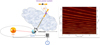 |
Fig. 1 Illustration of the pulsar signal from a binary pulsar to timing data products. The binary motion of the pulsar around the binary barycentre (BB) causes Doppler shift of pulsar spin frequency. The pulsar signal propagates through ionised interstellar medium and suffers dispersive delay, causing the low-frequency signal to be delayed more than the signal at higher frequency. The plot on the right demonstrates this effect for PSR J0737–3039A observed at the L band of the MeerKAT telescope (Hu 2023). The received signal is further transferred to the Solar System Barycentre (SSB), where the Doppler shift of Earth’s motion has to be corrected. |
2 Pulsar timing
In this section we provide an overview of pulsar timing observation and data processing routines. A schematic diagram is shown in Fig. 1. Pulsars are rotating neutron stars. As the pulsar rotates, a series of pulse signals from its magnetic poles travel through the ionised interstellar medium (IISM) before arriving at the radio telescope and being time-stamped by a maser clock. Due to the interaction with the ionised media, the radio waves suffer a frequency-dependent time delay with respect to the signal at infinite frequency of
 (1)
(1)
where 𝔇 is the dispersion constant defined as 1/(2.41000 × 10−4)MHz2pc−1cm3s in pulsar software (Manchester & Taylor 1972) and DM0 ≃ 48.9 pc cm−3 is the intrinsic DM of PSR J0737–3039A at the observing epoch. The dispersive time delay between two edge frequencies of the band ƒlow and ƒhigh is therefore (Lorimer & Kramer 2004):
 (2)
(2)
Since the time delay is inversely proportional to the square of the frequency, the effect is most prominent at lower frequencies, as illustrated in the plot on the right of Fig. 1. After compensating for the dispersive delay (‘de-dispersing’), one expects to see an aligned profile in frequency such as the left panel of Fig. 2.
Single pulses are generally weak and vary in shape. To obtain a significant and stable pulse profile for pulsar timing, the incoming pulses are channelised in frequency and coherently de-dispersed within each channel, before being folded at the topocentric pulsar period over a sub-integration interval (typically ~10 s). Pulsars have excellent rotational stability. However, if the pulsar is moving in a binary system, the observed pulsar spin frequency ν will be Doppler shifted as a function of the orbital phase. As we show in this paper, the combination of dispersive delay and Doppler shift can introduce various artefacts if the data are not processed adequately.
Due to Earth’s orbital and rotational motion in the Solar System, the time of arrival (TOA) of the pulsar signal received at the telescope (‘topocentric’) must be transformed to the inertial reference frame at the Solar System Barycentre (SSB). Similar to the binary pulsar, Doppler frequency shift of Earth’s motion has to be considered in addition to other barycentric corrections (see e.g. Lorimer & Kramer 2004, for a more complete overview).
Pulsar observing systems that produce phase-resolved averages of observed quantities, such as the Stokes parameters, require a model that predicts the pulse phase as a function of time. Evaluation of the physical timing model at every time sample is not computationally feasible; therefore, a polynomial is fit to the timing model and used to predict phase. For example, the timing program TEMPO2 (Nice et al. 2015) produces onedimensional polynomials ϕ(1)(t; ƒ0) that predict pulsar rotational phase as a function of topocentric time t at a single topocentric reference frequency ƒ0. In commonly used signal processing software such as DSPSR (van Straten & Bailes 2011)3, the phase predicted by ϕ(1)(t; ϕ0) is applied to all frequency channels that span the observed band. The dispersive delays between the frequency channels are corrected only after integrating over some period of time, T. In this case, the dedispersed pulse phase at time t and radio frequency ƒ is described by the following approximation, which can be compared to Eq. (27) of Hobbs et al. (2006, hereafter ‘HEM2006’).
 (3)
(3)
Here, v(1) = dϕ(1)/dt predicts the topocentric spin frequency of the pulsar at t and ƒ0; tmid is an epoch near the middle of the sub-integration; and ∆tDM corrects the dispersive delay between ƒ and ƒ0 ; this correction varies with time owing to the motion of the observatory with respect to the SSB. Equation (3) breaks down when the topocentric spin frequency of the pulsar varies significantly during either the sub-integration time T or the dispersive delay interval ∆tDM , whichever is greatest. An exact expression for a de-dispersed pulse phase is given by
![Mathematical equation: $\phi (t,f) = {\phi _{(1)}}\left( {t - \Delta {t_{{\rm{DM}}}}\left[ {t,f,{f_0}} \right];{f_0}} \right),$](/articles/aa/full_html/2025/02/aa53051-24/aa53051-24-eq4.png) (4)
(4)
Accurate calculation of the dispersive delay requires compensation of the Doppler shift due to the motion of the observatory with respect to the SSB, and this physical model can also be approximated by a best-fit polynomial. A similar approach is introduced by HEM2006, in which two-dimensional Chebyshev polynomials are used to predict pulse phase as a function of topocentric time and frequency. Commonly used signal processing software packages, such as DSPSR, PSRCHIVE and PRESTO, do not yet fully implement the required polynomials, and continue to use the approximation presented in Eq. (3). The artefacts caused by the difference between ф(t, f) and  are discussed and demonstrated using simulations in Sections 4 and 5.
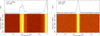 |
Fig. 2 Example of simulated pulsar data files as shown by pazi command of the PSRCHIVE software. The left panel shows the simulated data using the Double Pulsar profile and the right panel shows the simulated data using a broad Gaussian profile. |
Setup used to generate various datasets used in the current paper.
3 Pulsar data simulator
In the current paper we make extensive use of the python-based PULSAR SIGNAL Simulator (PSRSIGSIM) package, the main purpose of which is to produce realistic pulsar datasets. The details of the original version of the software developed by the North American Nanohertz Observatory for Gravitational Waves (NANOGrav) are described in Shapiro-Albert et al. (2021). We have kept the core of the native version; however, some of the modules have been modified to fit the purposes of our investigation4. In particular, the pieces of the code have been updated to achieve phase connection with ‘polyco’ and ‘T2predict’ phase predictors, based on TEMPO and TEMPO2 (Hobbs et al. 2006) pulsar timing software, respectively. For the rest of the paper the phase-connection has been implemented with the ‘polyco’ predictor, given that the complete timing model for the Double Pulsar is only available in TEMPO. See Section 6 for more details on phase connection.
The PSRSIGSIM has been used to create a series of phase- connected simulated pulsar observations. For this work, we have exclusively used the FILTERBANKSIGNAL class to produce channelised, time-resolved data cubes with pulsar observations folded modulo pulsar period. Thanks to built-in support of the PULSAR DATA TOOLBOX (PDAT, Hazboun & Shapiro-Albert 2020) the resulting data cubes are output in the PSRFITS format, which is compatible with the PSRCHIVE software (Hotan et al. 2004), most commonly used to analyse pulsar astronomical data. PSRSIGSIM produces one pulsar data file per observational epoch with a customised number of frequency channels, phase bins and time sub-integrations. The profile shape and pulsar ephemeris are also fully user definable. Examples of generated pulsar data files are demonstrated in Fig. 2. Although PSRSIGSIM software supports the creation of pulsar data files with frequency-evolving templates (through PORTRAIT class), in this work we ignore any possible profile shape change along the frequency band, both intrinsic and related to scattering in the IISM. We note that in reality profile changes will further complicate the situation.
The functionality of PSRSIGSIM is particularly when investigating the influence of various frequency-dependent effects on pulsar timing. In particular, in this paper we simulate apparent chromatic artefacts induced by the motion of a pulsar in a binary system, such as those that are observed in the real data of PSR J0737–3039A. To explore their nature and observational manifestation, a number of different pulsar ephemerides (e.g., with a pulsar in a circular or elliptical orbit) and profile shapes have been used. The setup has been adapted for each effect separately and is summarised in corresponding sections and Table 1.
4 Doppler effects from binary pulsars
4.1 Dispersive Doppler variation (DDV)
In this section, we show that the effect apparently observed by Ransom et al. (2004) in fact arises due to an unaccounted relativistic Doppler shift of pulsar spin frequency as the pulsar moves on its orbit in a binary system, which is practically equivalent to assuming a constant pulsar spin frequency over the orbit when computing the dispersive phase shift. The Doppler- shifted spin frequency observed at the observatory on Earth v(t) is related to the emission frequency v0 as
 (5)
(5)
where β(t) is the ratio of the radial velocity of the pulsar  and the speed of light c. It is assumed that
  if the pulsar is moving away from us. The pulse phase difference from dispersive delay
  is then given by the product of the dispersive delay time ∆tDM and the observed spin frequency v(t):
 (6)
(6)
However, if the data are de-dispersed using v0 (instead of vobs) as if the pulsar were fixed at the binary barycentre (as if ‘solitary’), this would then lead to an apparent DM of DM′ = DM0 + δDM, and a pulse phase difference
 (7)
(7)
If the phase shift caused by dispersion (Eq. (6)) is corrected without accounting for the Doppler shift of spin frequency (Eq. (7)), by equalling Eqs. (6) and (7), one obtains the apparent DM variation
 (8)
(8)
Using the Taylor expansion, we can simplify it to the first order as
 (9)
(9)
For PSR J0737−3039A, the orbital velocity is about a thousandth of the speed of light, given that the orbit is nearly edge on. The maximum DM variation is thus δDMmax ≃ 10−3 DM0 = 0.05 pc cm−3. This is consistent with the DM amplitude reported in Ransom et al. (2004). The occurrence of this error can also be expressed following Eq. (3) as:
 (10)
(10)
In order to reproduce the observed behaviour shown in Ransom et al. (2004), we simulated pulsar data files using the PSRSIGSIM software with the following setup. The profile and ephemeris are those of the Double Pulsar. The generated 4- minute data files have a time resolution of 10 seconds. The total bandwidth of 100 MHz is split into 200 channels with a central frequency of 452 MHz. Details of the simulation correspond to the Setting 1 described in Table 1. The pulsar software package PSRCHIVE corrects the frequency-dependent effects in relation to the centre frequency, while the version of Berkeley-Caltech Pulsar Machine (BCPM, Kaspi et al. 2004) used the highest frequency of the band as the reference value. Therefore, the total bandwidth of simulated data files is twice the bandwidth of the original observations. The upper part of the frequency was discarded later in the post-processing. The simulated data files were de-dispersed with a modified parameter file that did not contain the binary model (in other words we assumed that the spin frequency is constant over the binary orbit), which effectively introduce the effect of uncorrected orbital Doppler shift of the spin frequency. All other processing steps were performed with the re-installed original parameter file of J0737–3039A. The results are shown in Figs. 3 and 4. Fig. 3 presents the timing residuals in four different sub-bands as a result of the uncorrected Doppler effect, while the apparent DM measured from the simulated data is demonstrated in Fig. 4.
Therefore, as confirmed by the mathematics and further with simulations, the incomplete correction of the Doppler shift of the pulsar spin frequency, combined with the dispersive delay caused by the IISM, creates apparent DM variations of the required magnitude.
In the past, this problem has been diminished by splitting the timing data into narrow sub-bands and folding each sub-band using a one dimensional phase predictor computed with a reference frequency equal to the centre of the band. To demonstrate this, we divide these data (402–452 MHz) into 25 sub-bands, each with a bandwidth of 2 MHz, and calculate the time delays within the sub-bands using Eq. (6). The results are shown in Fig. 5, where the difference between the lower (upper) edge and the centre of the sub-bands is shown in red (blue) for all 25 subbands. The maximum amplitude corresponds to the sub-band with the lowest frequency. The error introduced by this effect is reduced from ~200 µs in Fig. 3 to a level of ~5 µs, which is well below the observational error of the pulse arrival time (~20 µs for the GBT data), and therefore has little impact on the timing precision. The bandwidth can be chosen in such a way that the time difference within the sub-bands is smaller than the observational error. This approach was employed in the analysis of the 16-yr data (Kramer et al. 2006, 2021), which helped to improve the timing precision before PSRCHIVE became available (while minimising the higher-order spectral smearing effect discussed in the following section). As PSRCHIVE already takes into account the Doppler effect of spin frequency properly, such apparent orbital DM variation should no longer be present. However, the effect may still occur when the data are processed by other software such as SIGPROC.
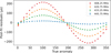 |
Fig. 3 Timing variations simulated by PSRSIGSIM software as a function of a true anomaly for 4×12.5 MHz sub-bands covering a 50 MHz band centered at 427 MHz. The setup repeats the one used in the Ransom et al. (2004). The apparent variations in timing residuals have the same magnitude of ~200 µs as reported by Ransom et al. (2004). |
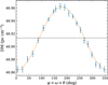 |
Fig. 4 Apparent DM variation reproduced by de-dispersing the simulated data with a non-binary model (shown as blue points), that is, ignoring the dispersive Doppler variation (DDV). The data are plotted against pulsar’s angular orbital position ψ = ω + θ (ω is the longitude of periastron and θ is the relativistic true anomaly) with respect to the ascending node. Both amplitude and phase are consistent with Fig. 2 in Ransom et al. (2004), given that ω ~ 80°. The dashed horizontal line indicates the DM used in the simulation, and the orange line represents the calculation with Eq. (9), which matches perfectly with the simulation. |
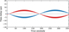 |
Fig. 5 Dispersive time delay within a narrow 2 MHz-band as a comparison to Fig. 3. For all 25 sub-bands, the time difference between the lower edge of the sub-band and the central frequency is shown in red, while the time difference between the upper edge and central frequency is shown in blue. The lower the frequency of the sub-band, the greater the amplitude of the time delay. As one data point is generated per subband for a given sub-integration, this adds a ~10 µs error to the data. |
4.2 Second-order dispersive Doppler effects
In addition to the first-order dispersive Doppler effect, DDV, two second-order effects of much smaller magnitude occur with the current data processing software and cause profile smearing. The magnitude of these effects can be estimated using the frequency-dependent difference between  and ф (Eqs. (3) and (4), respectively), which is approximated using the Taylor expansion of the phase predictor,
 (11)
(11)
where ∆t = t − tmid, such that the topocentric spin frequency is
 (12)
(12)
Ignoring any variation in the motion of the observatory during the sub-integration time, all dispersive Doppler smearing artefacts caused by the motion of the pulsar are described by the phase difference,
![Mathematical equation: $\matrix{ {\Delta \phi (t,f)} \hfill & { = \tilde \phi (t,f) - \phi (t,f)} \hfill \cr {} \hfill & { = \Delta {t_{{\rm{DM}}}}(t,f)\left[ {{{\ddot \phi }_0}\Delta t - {1 \over 2}{{}_0}\Delta {t^2} + \ldots } \right]} \hfill \cr {} \hfill & { - {1 \over 2}\Delta t_{{\rm{DM}}}^2(t,f)\left[ {{{\ddot \phi }_0} + \Delta t + \ldots } \right]} \hfill \cr {} \hfill & { + {1 \over 6}{{}_0}\Delta t_{{\rm{DM}}}^3(t,f) + \ldots } \hfill \cr } $](/articles/aa/full_html/2025/02/aa53051-24/aa53051-24-eq18.png) (13)
(13)
The leading term in this equation (proportional to ∆tDM) describes the temporal dispersive Doppler smearing (TDDS) effect, while the second term represents the spectral dispersive Doppler smearing (SDDS) effect. The magnitude and manifestation of these effects in pulsar timing data are discussed in the following sections.
4.2.1 Temporal dispersive Doppler smearing (TDDS)
Temporal dispersive Doppler smearing arises when the temporal variation of the Doppler-shifted pulsar spin frequency is neglected in the calculation and correction of the dispersive phase shift. This occurs whenever the average profile is integrated before the dispersive delay is corrected, and the amount of smearing increases with in tegration length.
At conjunction, where  , the total dispersive smearing over the sub-integration time T is approximately
 (14)
(14)
where v0 = v(1)(tmid, f0) is the pulsar spin frequency at the midtime of the sub-integration, ar is the radial acceleration of the pulsar, and c is the speed of light. Although maximal at conjunction, this smearing is also symmetric for either a circular orbit or an elliptical orbit for which periastron is at conjunction (for the first half of T, ∆t < 0, and for the second half, ∆t > 0). Therefore, in such cases, the impact on arrival times is minimal at conjunction. In contrast, at the (ascending and descending) nodes, where  , TDDS is dominated by the
  term and varies quadrat- ically with ∆t. Therefore, the smearing is asymmetric and the impact on arrival times is maximal at the nodes.
Predicting the impact of smearing on arrival times is not trivial due to its strong dependence on the intrinsic shape of the average pulse profile. However, estimating the amount of smearing still provides a useful order of magnitude estimate. After 5 minutes of integration using a polynomial computed for f0 = 815 MHz to fold a signal at f = 570 MHz, there is ~70 µs of smearing in PSR J0737–3039A. This second-order smearing is eliminated by correcting the dispersive delay before any temporal-averaging is applied.
To demonstrate this effect, we simulate pulsar data files at frequencies similar to the UHF band of MeerKAT (570– 1060 MHz) with different profiles and orbital eccentricities. The specification of the simulated dataset is described by Setting 2a in Table 1. The data were folded every 30 minutes without prior de-dispersion, which would otherwise have mitigated the effect. Figs. 6 and 7 show how the effect alters the PSR J0737–3039A profile and a narrow Gaussian profile (width-period ratio of 0.006) at a chosen orbital phase near the superior conjunction (ranging from 88° to 160°) where the smearing effect is prominent. A circular orbit is assumed in both cases. It can be seen that after folding the pulse profiles (black lines in the left panels) are broadened at lower and upper parts of the band, compared to the standard template in red. The difference in the black and red profiles is shown on the right panels.
For each of these profile shapes, Fig. 8 shows the arrival-time residuals after fitting for DM. For a relatively wide profile such as that of J0737–3039A, the apparent DM can be effectively removed by the fit. As a result, nearly flat residuals as a function of frequency are observed in Fig. 8a. Similar results are obtained in a simulation with a broad Gaussian profile (width-period ratio of 0.1). This suggests that for wide pulse profiles, TDDS leads to residuals that can be reabsorbed with an inverse quadratic dependence on the observation frequency, which results in biased DM estimates.
However, for narrow profiles, the residuals have a different functional form, as is illustrated in Fig. 8b. In contrast to the broad profile case, significant spectral structure remains in the residuals after fitting for DM. From Fig. 7 one can see that the profile is predominantly smeared to the left (right) at the lower (upper) part of the frequency band. Therefore, it is reasonable to expect that the residuals should follow the same "DM-like" trend as seen in Fig. 8a. This is indeed the case for residuals ≳660 MHz. However, below ~660 MHz, although the smearing is wider on the left, it has a higher peak on the right (see Fig. 7). This asymmetric smearing causes the template to be matched to the peak component on the right-hand side of the smeared profile, corresponding to positive residual delay. This anomaly is not observed when the width of the pulse is substantially greater than the timescale of the TDDS. Despite this anomaly, the resulting apparent DM variations are similar for different pulse widths.
In Fig. 9 we show the apparent DM variation caused by orbital profile smearing using J0737–3039A’s profile for different orbital eccentricities. A circular orbit leads to a sinusoidal variation (blue), whereas the Double Pulsar orbit (e = 0.088) results in a slightly asymmetric variation, which is consistent with what has been seen with MeerKAT when processing the data in a similar fashion. The amplitude of this effect is an order of magnitude smaller than the DDV described in Section 4.1 and found in Ransom et al. (2004). As the eccentricity increases, the variation becomes more dramatic in amplitude, as indicated by the green points in Fig. 9 for e = 0.6.
To summarise, for highly relativistic binaries, observations with a sufficiently wide band could result in orbital phase-dependent profile smearing that can cause apparent phasedependent DM variations, if TDDS is not taken into account. Such smearing of a profile can be eliminated if the data are de-dispersed first before integration.
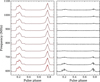 |
Fig. 6 Profile comparison using the J0737–3039A profile with a circular orbit. The black lines in the left panel show the profile of processed data at different frequencies as compared to the standard template in red, and the right panel shows the difference between the smeared profile and the standard profile (magnified by five times) without any phase shift. |
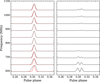 |
Fig. 7 Same as Fig. 6 but for a narrow Gaussian profile with a circular orbit. We note that the pulse phase is zoomed to show the details of pulse profile and that the residuals in the right panel are not magnified. |
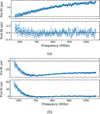 |
Fig. 8 Pre-fit and post-fit residuals after fitting for DM shown in relation to frequency. The figures show the same orbital phase (ψ ~ 130°) in a circular orbit but for different pulse profiles. (a) J0737–3039A profile (see Fig. 6), residuals can mostly be absorbed by fitting DM. (b) Narrow Gaussian profile (see Fig. 7), only residuals ≳660 MHz are absorbed by fitting for the DM. |
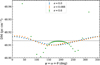 |
Fig. 9 Apparent DM variation caused by orbital profile smearing for different eccentricities using the J0737–3039A profile. |
4.2.2 Spectral dispersive Doppler smearing (SDDS)
In contrast to TDDS, the SDDS effect arises when spectral variation of the Doppler-shifted pulsar spin frequency across the observed bandwidth is neglected when computing and correcting the dispersive phase shift. The sign and magnitude of the effect depends on orbital phase and is independent of integration length.
For highly relativistic systems such as the Double Pulsar, due to a significant change in the position of the pulsar in its orbit during the dispersive delay time, pulses which are received simultaneously at different frequencies were originally emitted at different orbital phases. However, the current implementation of PSRCHIVE uses phase predictions at a single central frequency. When this predictor is used to fold data at other frequencies, it effectively neglects the difference in apparent spin frequency between different bands and causes profile smearing after averaging in frequency. This effect was commonly misaccepted by the community5 as an explanation for the DM variations seen in Ransom et al. (2004).
More specifically, if the data are folded with a slightly higher spin frequency (i.e. shorter spin period), the profile shifts to the right, and vice versa. A schematic of pulse broadening due to folding with wrong spin periods is demonstrated in Fig. 10. At the conjunctions (ψ = 90°/270º), when individual profiles move both left- and rightwards, the average profile becomes broadened on both sides and the impact on the arrival time is minimal. While at the ascending and descending nodes (ψ = 0°/180°), the profiles shift towards one direction, and therefore the impact on the arrival time is maximal. As the effect is most prominent at low frequencies, it is covariant with scattering caused by turbulent IISM plasma.
The spectral smearing expansion in Eq. (13) is dominated by the leading  term; therefore, the SDDS is maximal at conjunction, where
 (15)
(15)
When using a polynomial computed for f0 = 815 MHz to fold a signal at f = 570 MHz, the maximal inaccuracy is ~37 ns for PSR J0737–3039A. Compared to TDDS, the SDDS is not related to integration time, but, because it is proportional to  , it becomes much more significant at lower radio frequency. For example, even though this effect is three orders of magnitude smaller than the temporal smearing at the UHF band and does not affect the timing precision, it becomes the dominant effect at low frequencies, as shown in Section 4.2.3.
From a technical point of view, the SDDS can also be avoided by applying the de-dispersion routine prior to averaging. In this case, data at all observational frequencies effectively correspond to the same orbital phase so that the same spin frequency can be applied.
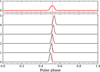 |
Fig. 10 Schematic of folding with wrong spin periods. The resulted averaged profile (red) becomes broader and flatter. Viewing from top down, folding with a long spin period shifts the centre of the averaged profile to the left; from bottom up, folding with a short spin period shifts the averaged profile to the right. |
4.2.3 Simulations for the SKA and separating the two effects at low frequencies
Both SDDS and TDDS lead to a frequency dependent shift that can manifest itself as orbital DM variations (especially for broad pulse profiles). Therefore, the two effects are highly covariant and difficult to disentangle. The most striking difference is evident from the Eqs. (14) and (15): in contrast to spectral smearing, temporal smearing depends on integration time and, therefore, there are some regimes where one is dominant over the other.
We plot the maximum magnitude of these two effects (over the orbital phase) in Fig. 11 for binaries with different orbital periods (i.e. accelerations). The left axis shows the smearing for the case of SKA-Low, whereas the right axis shows the values for the SKA-Mid, which is ~60 times smaller. The smearing increases significantly with acceleration (for both effects) and sub-integration length (for temporal smearing). The magnitude of these two effects is approximately equal when the sub-integration length T approaches half of the dispersive delay time. At SKA-Mid, the induced timing residuals are dominated by the temporal smearing starting from T = 0.6 s, as well as for the UHF band as showed in Sections 4.2.1 and 4.2.2. However, at SKA-Low, where the dispersive delay is much longer, the smearing is dominated by the spectral Doppler effect when T < 38 s.
In order to separate these two effects and illustrate the SDDS, we simulate SKA-Low data (50–350 MHz, see Setting 2b in Table 1) with different sub-integration lengths. The comparison of timing residuals with different T is shown in Fig. 12. For sub-integration time (T = 10, 15, 30 s) smaller than half of the dispersive delay time (38 s), the magnitude of residuals remains the same, indicating that the smearing is dominated by SDDS. The lower panel shows the timing residuals for T = 10 s for four different orbital phases, which agrees with the theoretical prediction of Eq. (15) for SDDS (grey lines). In contrast, when the sub-integration time is much longer than half of the dispersive delay time (T = 100 s), the magnitude of residuals increases and spreads around the mean. This different observing manifestation comes from the TDDS. In Fig. 13 we show the spectrum of the data for the latter case where the pulse is smeared in both directions at the lowest frequencies, resembling the ‘Eiffel Tower’.
At higher frequency such as SKA-Mid (350–1450 MHz, see Setting 2c in Table 1), the effect is dominated by TDDS and is demonstrated in Fig. 14 with sub-integration time of 500 s, 900 s and 1000 s, respectively. The timing residuals caused by TDDS increase with sub-integration length at the given orbital phase, with the most prominent effect occurring at the lower part of the band as predicted by Eq. (14).
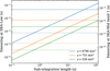 |
Fig. 11 Maximum smearing with respect to sub-integration length for SKA-Low (left y-axis) and SKA-Mid (right y-axis) calculated using Eqs. (14) and (15), assuming the spin period and DM of PSR J0737–3039A, a mass of 1.4 M⊙, and circular orbits. The blue, orange, and green lines denote orbital periods of 15 min, 1 h, and 2.45 h (PSR J0737–3039A), respectively, with the maximum acceleration labelled. The SDDS (dashed lines for SKA-Low and dotted lines for SKA-Mid) dominates over the TDDS (solid lines) when the sub-integration length is smaller than half of the dispersive delay time (∆tDM = 76.1 s for SKA-Low and ∆tDM = 1.2 s for SKA-Mid), and vice versa. |
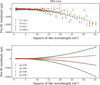 |
Fig. 12 Timing residuals plotted against wavelength squared for simulated SKA-Low data. Upper panel: Timing residuals for a chosen epoch perturbed by SDDS and TDDS different sub-integration times T. For T = 10, 15, 30 s, the effect of SDDS prevails the TDDS and the residuals are consistent; while for T = 100 s, the TDDS dominates and distorts the signal at lower part of the frequency band (see Fig. 13) and increases the residuals. Lower panel: Timing residuals for T = 10 s dominated by the SDDS. The colours correspond to different orbital phases ψ. Grey lines illustrate the theoretical magnitude of the SDDS predicted by Eq. (15). |
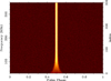 |
Fig. 13 The TDDS effect in the simulated SKA-Low data for T = 100 s to make the effect more prominent. The corresponding residuals are demonstrated in Fig. 12. |
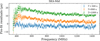 |
Fig. 14 Timing residuals of the TDDS effect simulated for the SKA- Mid data (Setting 2b). The magnitude of the effect gradually increases with the sub-integration time T as predicted by Eq. (14). |
5 Topocentric Doppler effects
In the previous section we discussed three dispersive Doppler artefacts related to the pulsar’s orbital motion. Here we complete this discussion by also considering the observatory’s motion relative to the SSB and its related impact.
5.1 Topocentric dispersive Doppler variation (TopoDDV)
In Eqs. (3) and (4), time and frequency are specified in the topocentric reference frame of the observatory. However, dispersion takes place in the rest frame of the IISM, which assumed to have constant velocity with respect to the SSB. Therefore, before computing the (topocentric) dispersive delay ∆tDM, topocentric frequencies are first converted to barycentric frequencies, then the resulting barycentric delay is converted to a topocentric delay as follows. Given the velocity of the observatory with respect to the SSB projected onto the line of sight to the pulsar, υtopo(t), topocentric frequency f is related to barycentric frequency fSSB by f = [1 + βtopo(t)] fSSB, where βtopo(t) = υtopo(t)/c is positive when the observatory is moving toward the pulsar. Similarly, any signal propagation interval (such as wave period or dispersive delay) is transformed from the rest frame of the SSB to that of the observatory by ∆t = ∆tSSB [1 + βtopo(t)]−1. Combining the transformations of radio frequency and time interval yields the following expression for the topocentric DDV (TopoDDV), corrected for the motion of the observatory with respect to the SSB,
![Mathematical equation: $\matrix{ {\Delta {t_{{\rm{DM}}}}\left( {t,f,{f_0}} \right)} \hfill & { = \Delta {t_{{\rm{DM}},{\rm{SSB}}}}\left( {{f_{{\rm{SSB}}}},{f_{0,{\rm{SSB}}}}} \right){{\left[ {1 + {\beta _{{\rm{topo}}}}(t)} \right]}^{ - 1}}} \hfill \cr {} \hfill & { = D\left[ {f_{{\rm{SSB}}}^{ - 2} - f_{0,{\rm{SSB}}}^{ - 2}} \right]{{\left[ {1 + {\beta _{{\rm{topo}}}}(t)} \right]}^{ - 1}}} \hfill \cr {} \hfill & { = D\left( {{f^{ - 2}} - f_0^{ - 2}} \right)\left[ {1 + {\beta _{{\rm{topo}}}}(t)} \right],} \hfill \cr } $](/articles/aa/full_html/2025/02/aa53051-24/aa53051-24-eq26.png) (16)
(16)
where D = 𝒟 × DM. In the current version of PSRCHIVE, the barycentric correction is disabled by default, and can be enabled by setting Dispersion::barycentric_correction = 1 in the psrchive.cfg file. When enabled, the correction is approximated by
![Mathematical equation: $\Delta {t_{{\rm{DM}}}}\left( {t,f,{f_0}} \right) \simeq D\left( {{f^{ - 2}} - f_0^{ - 2}} \right){\left[ {1 - {\beta _{{\rm{topo}}}}(t)} \right]^{ - 1}},$](/articles/aa/full_html/2025/02/aa53051-24/aa53051-24-eq27.png) (17)
(17)
which is valid for small βtopo(t). If this correction is not enabled, Earth’s orbital velocity will induce an apparent annual modulation of DM with a maximum relative amplitude of δDMmax/DM ≃ 10−4 for pulsars near the ecliptic plane. A much smaller apparent diurnal variation of DM due to Earth’s rotation has a maximum relative amplitude of δDMmax/DM ≃ 10−6 for a pulsar and observatory near the equator.
5.2 Topocentric temporal dispersive Doppler smearing (TopoTDDS)
When phase is predicted using Eq. (3), the variation of the velocity of the observatory over the sub-integration time also leads to phase drift and profile smearing, as demonstrated in Section 7 of HEM2006. Including this variation in Eq. (13) gives rise to an additional term:
![Mathematical equation: $\matrix{ {\Delta {\phi _{{\rm{topo}}}}(t,f)} & { = {{\dot \phi }_0}\left[ {\Delta {t_{{\rm{DM}}}}\left( {t,f,{f_0}} \right) - \Delta {t_{{\rm{DM}}}}\left( {{t_{{\rm{mid}}}},f,{f_0}} \right)} \right]} \cr {} & { = {v_0}D\left( {{f^{ - 2}} - f_0^{ - 2}} \right)\left[ {{\beta _{{\rm{topo}}}}(t) - {\beta _{{\rm{topo}}}}\left( {{t_{{\rm{mid}}}}} \right)} \right].} \cr } $](/articles/aa/full_html/2025/02/aa53051-24/aa53051-24-eq28.png) (18)
(18)
Over the duration of the sub-integration T, the total smearing is, to the first order,
 (19)
(19)
where atopo is the acceleration of the observatory with respect to the SSB, projected onto the line of sight to the pulsar. For a pulsar in the ecliptic plane with DM=50 pc cm−3, integrating for T = 30 s using a polynomial computed for f0 = 200 MHz to fold a signal at f = 50 MHz results in maximum smearing of ~46 ns. In MeerKAT L-band observations of PSR J0737–3039A, the effect is two orders of magnitude smaller.
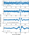 |
Fig. 15 Timing residuals of the simulated data files versus orbital phase for binary systems with orbital periods of 4.5 h, 3 h, 2.45 h, and 1 h. The spiky features appearing at the superior conjunction (ψ = 90°) demonstrate the limitations of the current software, in this case, the ‘polyco’ predictor. The simulation was done with TZNSPAN=3 min and 20 coefficients. |
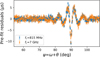 |
Fig. 16 Same as Fig. 15 but for the Double Pulsar with observations simulated at two remote radio frequencies of 815 MHz (blue) and 7000 MHz (orange). The figure clearly shows that the systematic issue due to folding is independent of observational frequency. |
6 Folding issues with phase predictors
Another systematic issue that arises when timing highly relativistic pulsar binaries is due to the limited accuracy of current phase predictors. When averaging the data in frequency or time, PSRCHIVE and DSPSR do not use the pulsar ephemeris directly, but rather use pulse phase predictions. Commonly, the pulse phase prediction information is supplied by a predictive polynomial file derived from the pulsar ephemeris, which are ‘polyco’ or ‘T2predict’ files generated using the pulsar timing software TEMPO and TEMPO2, respectively. This contains a set of polynomial coefficients that describe the pulse phase and spin frequency for a given observation frequency and time range. The parameter TZNSPAN defines the valid time span covered by each unique set of coefficients. One should emphasise that the predictor does not represent the exact timing solution, but rather the approximation of it using polynomial/Chebyshev expansion. These approximated polynomials generally describe the timing solution well, but fail for relativistic binaries especially at the superior conjunction due to the sharpness of the Shapiro delay, which follows a natural logarithm (Blandford & Teukolsky 1976; Damour & Deruelle 1986):
 (20)
(20)
![Mathematical equation: $\matrix{ {{\Lambda _u}} & { = 1 - e\cos u - s[\sin \omega (\cos u - e)} \cr {} & {\left. { + {{\left( {1 - {e^2}} \right)}^{1/2}}\cos \omega \sin u} \right].} \cr } $](/articles/aa/full_html/2025/02/aa53051-24/aa53051-24-eq31.png) (21)
(21)
The parameters r and s are the post-Keplerian parameters representing the ‘range’ and ‘shape’ of the Shapiro time delay as the pulsar signal passes in the vicinity of the companion, which can be measured using pulsar timing. e is the orbital eccentricity, u is the relativistic eccentric anomaly, and ω is the longitude of periastron. The limitation of polynomial approximation has been known for a long time, which can in principle affect all timing parameters, but is most easily seen in the Shapiro delay parameters. As noted by Hu et al. (2022), inappropriate choice of a predictor and relevant parameters (TZNSPAN and the number of polynomial coefficients – ‘TZNCOEF’) can cause bias in the measurements of Shapiro delay parameters.
In order to demonstrate the difference between the exact timing solution and the ‘polyco’-predicted phase, we simulate a series of data files with the setup listed in Table 1. For comparison purposes, we generate pulsar data files with different orbital periods, and here we choose to present four cases: 4.5 h, 3 h, 2.45 h (i.e. the Double Pulsar) and 1 h. For all four cases the resolution of the predictor, defined by the TZNSPAN parameter, is fixed to 3 min. After generation, fully resolved data files are de-dispersed and frequency-averaged. The pulsar data files are generated with ultra-high signal-to-noise ratio, so their precision exceeds that of data from existing telescopes. Given that PSRSIGSIM generates pulsar data files based on the polynomial expansion of the timing solution (predictor), the discrepancies of interest should be visible in the residuals after subtracting the best-fit timing model and are indeed shown in Fig. 15. As expected the difference is most prominent at orbital phase ψ = 90°, which corresponds to the superior conjunction of the binary system. Fig. 15 also clearly shows that the systematic error increases as the orbital period decreases. One should note here that the considered effect does not depend on observational frequency and bandwidth, as it is demonstrated in Fig. 16.
Such discrepancies are not immediately visible in real observations, but will propagate in the timing analysis at specific stages of post-processing. To be more precise, systematic error arises at the superior conjunction of highly relativistic binaries, when forming the sub-integrated data with, for example, DSPSR software, which uses polynomial expansion in its base. To simulate the effect as it appears in the real data, we create pulsar data files with 1 s sub-integration length and 1 min time resolution for the predictor (defined by the parameter TZNSPAN), which is the smallest possible TZNSPAN that is compatible with the PSRCHIVE software. This allows us to mimic realistic observations as closely as possible. Data were simulated for PSR J0737–3039A and a fake binary pulsar with an orbital period of 4.5 h (Setting 3b in Table 1). When averaging the data only in frequency with TZNSPAN=1 min, the systematic error of interest is not visible in either system. However, if the resolution of the ‘polyco’ predictor in the original file is reduced (i.e. a larger TZNSPAN) and the sub-integration length of the data is increased, the systematic effect appears.
As demonstrated in Fig. 17, the longer the sub-integration length and the worse the resolution of the phase predictor, the larger the effect. Specifically, the systematic error of interest is shown for two different values of TZNSPAN, 1 min and 1 h, and two different time-averaging factors, which are 60 and 120, corresponding to 1 min and 2 min length of sub-integration. For the Double Pulsar, the size of the effect is as high as ~5 µs for 30-s sub-integration time and TZNSPAN=1 min, which is still below the root mean square (RMS) of MeerKAT data with the same sub-integration (Hu et al. 2022). However, it can bias the Shapiro parameter measurements and is expected to be more visible in a few years with the SKA. In Table 2 we estimate the expected bias in the Shapiro parameters s and r for MeerKAT and the SKA-Mid at different stages: the Array Assembly (AA)* in 2028 and the final AA46. Although the accuracy of long-term post- Keplerian parameters is not studied in this work, it is expected that they will also be affected by inaccuracies in the modelling of the Shapiro delay.
Although the Double Pulsar is not in the field of view of FAST, currently the most sensitive radio telescope, other relativistic binaries such as PSR J1946+2052 may face the same problem. For sensitive telescopes such as FAST and the SKA, shorter integration times can be used to achieve the target sensitivity. Despite this, due to the improved sensitivity of these instruments, the folding problem will be even more evident due to the limited accuracy of the polynomial approximation and the limited implementation of the TZNSPAN parameter in the current software. In order to mitigate this folding artefact, the temporal resolution of the phase predictor and/or the approximation method needs to be improved.
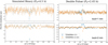 |
Fig. 17 Timing residuals of the simulated data files as a function of the orbital phase. A fictional binary with orbital period Pb = 2.45 h is shown on the left and the Double Pulsar is shown on the right. For all cases the original time resolution of the generated data files is TZNSPAN=1 min. Results with the originally installed 1-min resolution ‘polyco’ predictor are in orange, while in blue colour the results with re-installed ‘polyco’ with TZNSPAN=1 h resolution are shown. The upper panel shows the residuals after folding the originally generated fits files and reducing the time resolution by a factor of 60 (so that the resultant time resolution of the files is 1 min). The bottom panel is the same, but the time-averaging factor is 120 (2 min). The spiky features at phase ~0.25 represent limitations of the ‘polyco’ predictor, and become more pronounced as the time resolution of the predictor deteriorates and the sub-integration time (‘tsub’) increases. The effect is amplified for more relativistic binaries. |
Estimated bias in Shapiro parameters s and r for MeerKAT and the SKA based on simulated data.
List of all artefacts discussed in this paper along with their causes, manifestations, and solutions.
7 Summary and discussion
In this paper, we discussed several data processing issues that could arise in compact binary pulsar systems and summarised their causes, manifestations and solutions in Table 3.
Firstly, we have appropriately addressed the nature of the apparent DM variation seen in Ransom et al. (2004). For the first time, we have used mathematical expressions and simulations to show that the effect is due to an unaccounted first-order dispersive Doppler effect, the DDV. This Doppler shift of spin frequency has been implemented in the computation of dispersive phase shift in commonly used pulsar processing software PSRCHIVE and DSPSR, so such artefacts should not occur when processing the data with these tools.
Secondly, we have looked at two second-order dispersive Doppler effects that could cause orbital dependent profile smearing and mimic DM variation. TDDS occurs when a constant spin frequency is used to correct dispersion over the duration of the sub-integration time, whereas SDDS occurs when a constant spin frequency is applied over the observed bandwidth when computing the dispersive delay. Although the manifestations of both effects are similar, TDDS dominates over SDDS unless for observations at very low frequencies. Therefore in Section 4.2.3, we considered the special case of observing relativistic pulsar binaries using SKA-Low (50–350 MHz). At these low radio frequencies, for a pulsar in a circular orbit with a period of 1 h, folding with a one-dimensional phase predictor will result in significant TDDS of the order of 1 ms per 5 s of integration and SDDS of the order of 10 ms. A pulsar in an orbit with a period of 15 min will suffer TDDS of the order of 1 ms for each second of integration and SDDS of the order of 100 ms. Both TDDS and SDDS can be prevented, however, by de-dispersing the data prior to time integration (e.g. removing the inter-channel dispersive delays with ‘-K’ option in DSPSR). In addition, SDDS can also be avoided by utilising a two-dimensional phase predictor (or equivalent).
Finally, we have shown that the current folding techniques with polynomial approximation fail to describe the Shapiro delay with sufficient accuracy for compact binaries with <4 h edge-on orbit and could cause problems in the measurements of Shapiro delay parameters. As Shapiro delay parameters are often measured with high precision in a short timescale compared to other post-Keplerian parameters, they play important roles in testing gravity (Freire & Wex 2024), measuring neutron star masses and moment of inertia (Hu et al. 2020; Hu & Freire 2024), and subsequently help to constrain the equation of state of matter at supranuclear densities. This is not only relevant to the Double Pulsar, but also to other compact binaries, such as the 1.88 h-orbit double neutron star system PSR J1946+2052. Ongoing pulsar surveys are expected to discover more binary pulsar systems with tighter orbits, where the limitation of polynomial approximation becomes even more prominent. Such previously undetectable artefacts will become more visible with the everimproving sensitivity of the radio facilities. In particular, the FAST and the SKA (under construction) are expected to be significantly affected by these signatures and potentially limit the accuracy of timing parameters and consequently gravity tests. Therefore, a more accurate phase predictor is indispensable to minimise the systematic error in data processing and take the precision of gravity tests and the study of extreme matter to new heights.
Acknowledgements
We thank the anonymous referee for valuable and constructive feedback. We are grateful to Ramesh Karuppusamy for fruitful discussions and careful reading of the manuscript. HH acknowledges constant support from the Max Planck Society and funding by the MPG-CAS LEGACY collaboration. NKP is funded by the Deutsche Forschungsgemeinschaft (DFG, German Research Foundation)– Projektnummer PO 2758/1–1, through the Walter–Benjamin programme.
References
- Blandford, R., & Teukolsky, S. A. 1976, ApJ, 205, 580 [Google Scholar]
- Breton, R. P., Kaspi, V. M., Kramer, M., et al. 2008, Science, 321, 104 [NASA ADS] [CrossRef] [Google Scholar]
- Burgay, M., D’Amico, N., Possenti, A., et al. 2003, Nature, 426, 531 [NASA ADS] [CrossRef] [Google Scholar]
- Cameron, A. D., Champion, D. J., Kramer, M., et al. 2018, MNRAS, 475, L57 [NASA ADS] [CrossRef] [Google Scholar]
- Damour, T., & Deruelle, N. 1986, Ann Inst. Henri Poincaré (A) Phys. Théor., 44, 263 [Google Scholar]
- Einstein, A. 1915, Sitzungsberichte der Königlich Preussischen Akademie der Wissenschaften, 844 [Google Scholar]
- Freire, P. C. C., & Wex, N. 2024, Liv. Rev. Relativ., 27, 5 [NASA ADS] [CrossRef] [Google Scholar]
- Hazboun, J. S., & Shapiro-Albert, B. 2020, https://doi.org/10.5281/zenodo.4088660 [Google Scholar]
- Hobbs, G. B., Edwards, R. T., & Manchester, R. N. 2006, MNRAS, 369, 655 [Google Scholar]
- Hotan, A. W., van Straten, W., & Manchester, R. N. 2004, PASA, 21, 302 [Google Scholar]
- Hu, H. 2023, PhD thesis, University of Bonn, Germany [Google Scholar]
- Hu, H., & Freire, P. C. C. 2024, Universe, 10, 160 [CrossRef] [Google Scholar]
- Hu, H., Kramer, M., Wex, N., Champion, D. J., & Kehl, M. S. 2020, MNRAS, 497, 3118 [NASA ADS] [CrossRef] [Google Scholar]
- Hu, H., Kramer, M., Champion, D. J., et al. 2022, A&A, 667, A149 [NASA ADS] [CrossRef] [EDP Sciences] [Google Scholar]
- Hulse, R. A., & Taylor, J. H. 1975, ApJ, 195, L51 [NASA ADS] [CrossRef] [Google Scholar]
- Kaspi, V. M., Ransom, S. M., Backer, D. C., et al. 2004, ApJ, 613, L137 [NASA ADS] [CrossRef] [Google Scholar]
- Kramer, M., Stairs, I. H., Manchester, R. N., et al. 2006, Science, 314, 97 [NASA ADS] [CrossRef] [Google Scholar]
- Kramer, M., Stairs, I. H., Manchester, R. N., et al. 2021, Phys. Rev. X, 11, 041050 [NASA ADS] [Google Scholar]
- Lorimer, D. R., & Kramer, M. 2004, Handbook of Pulsar Astronomy, 4 [Google Scholar]
- Lower, M. E., Kramer, M., Shannon, R. M., et al. 2024, A&A, 682, A26 [NASA ADS] [CrossRef] [EDP Sciences] [Google Scholar]
- Lyne, A. G., Burgay, M., Kramer, M., et al. 2004, Science, 303, 1153 [CrossRef] [PubMed] [Google Scholar]
- Manchester, R. N., & Taylor, J. H. 1972, Astrophys. Lett., 10, 67 [NASA ADS] [Google Scholar]
- Nice, D., Demorest, P., Stairs, I., et al. 2015, Tempo: Pulsar timing data analysis, Astrophysics Source Code Library [record ascl:1509.002] [Google Scholar]
- Özel, F., & Freire, P. 2016, ARA&A, 54, 401 [Google Scholar]
- Ransom, S. M., Backer, D. C., Demorest, P., et al. 2004, arXiv e-prints [arXiv:astro-ph/0406321] [Google Scholar]
- Shapiro, I. I. 1964, Phys. Rev. Lett., 13, 789 [Google Scholar]
- Shapiro-Albert, B. J., Hazboun, J. S., McLaughlin, M. A., & Lam, M. T. 2021, Astrophys. J., 909, 219 [NASA ADS] [CrossRef] [Google Scholar]
- Stovall, K., Freire, P. C. C., Chatterjee, S., et al. 2018, ApJ, 854, L22 [NASA ADS] [CrossRef] [Google Scholar]
- Taylor, J. H., & Weisberg, J. M. 1982, ApJ, 253, 908 [NASA ADS] [CrossRef] [Google Scholar]
- Taylor, J. H., & Weisberg, J. M. 1989, ApJ, 345, 434 [NASA ADS] [CrossRef] [Google Scholar]
- Taylor, J. H., Fowler, L. A., & McCulloch, P. M. 1979, Nature, 277, 437 [NASA ADS] [CrossRef] [Google Scholar]
- van Straten, W., & Bailes, M. 2011, PASA, 28, 1 [Google Scholar]
- Wex, N., & Kramer, M. 2020, Universe, 6, 156 [NASA ADS] [CrossRef] [Google Scholar]
See comments uploaded with Ransom et al. (2004).
A digital signal processing software for filterbank pulsar data.
The original version of the code is publicly available through https://github.com/PsrSigSim/PsrSigSim, while the modified python library can be downloaded via https://gitlab1.mpifr-bonn.mpg.de/nata/psrsigsiml_mpifr_gitlab.git
See again comments uploaded with Ransom et al. (2004).
See https://www.skao.int/en for updates.
All Tables
Estimated bias in Shapiro parameters s and r for MeerKAT and the SKA based on simulated data.
List of all artefacts discussed in this paper along with their causes, manifestations, and solutions.
All Figures
|
Fig. 1 Illustration of the pulsar signal from a binary pulsar to timing data products. The binary motion of the pulsar around the binary barycentre (BB) causes Doppler shift of pulsar spin frequency. The pulsar signal propagates through ionised interstellar medium and suffers dispersive delay, causing the low-frequency signal to be delayed more than the signal at higher frequency. The plot on the right demonstrates this effect for PSR J0737–3039A observed at the L band of the MeerKAT telescope (Hu 2023). The received signal is further transferred to the Solar System Barycentre (SSB), where the Doppler shift of Earth’s motion has to be corrected. |
| In the text | |
|
Fig. 2 Example of simulated pulsar data files as shown by pazi command of the PSRCHIVE software. The left panel shows the simulated data using the Double Pulsar profile and the right panel shows the simulated data using a broad Gaussian profile. |
| In the text | |
|
Fig. 3 Timing variations simulated by PSRSIGSIM software as a function of a true anomaly for 4×12.5 MHz sub-bands covering a 50 MHz band centered at 427 MHz. The setup repeats the one used in the Ransom et al. (2004). The apparent variations in timing residuals have the same magnitude of ~200 µs as reported by Ransom et al. (2004). |
| In the text | |
|
Fig. 4 Apparent DM variation reproduced by de-dispersing the simulated data with a non-binary model (shown as blue points), that is, ignoring the dispersive Doppler variation (DDV). The data are plotted against pulsar’s angular orbital position ψ = ω + θ (ω is the longitude of periastron and θ is the relativistic true anomaly) with respect to the ascending node. Both amplitude and phase are consistent with Fig. 2 in Ransom et al. (2004), given that ω ~ 80°. The dashed horizontal line indicates the DM used in the simulation, and the orange line represents the calculation with Eq. (9), which matches perfectly with the simulation. |
| In the text | |
|
Fig. 5 Dispersive time delay within a narrow 2 MHz-band as a comparison to Fig. 3. For all 25 sub-bands, the time difference between the lower edge of the sub-band and the central frequency is shown in red, while the time difference between the upper edge and central frequency is shown in blue. The lower the frequency of the sub-band, the greater the amplitude of the time delay. As one data point is generated per subband for a given sub-integration, this adds a ~10 µs error to the data. |
| In the text | |
|
Fig. 6 Profile comparison using the J0737–3039A profile with a circular orbit. The black lines in the left panel show the profile of processed data at different frequencies as compared to the standard template in red, and the right panel shows the difference between the smeared profile and the standard profile (magnified by five times) without any phase shift. |
| In the text | |
|
Fig. 7 Same as Fig. 6 but for a narrow Gaussian profile with a circular orbit. We note that the pulse phase is zoomed to show the details of pulse profile and that the residuals in the right panel are not magnified. |
| In the text | |
|
Fig. 8 Pre-fit and post-fit residuals after fitting for DM shown in relation to frequency. The figures show the same orbital phase (ψ ~ 130°) in a circular orbit but for different pulse profiles. (a) J0737–3039A profile (see Fig. 6), residuals can mostly be absorbed by fitting DM. (b) Narrow Gaussian profile (see Fig. 7), only residuals ≳660 MHz are absorbed by fitting for the DM. |
| In the text | |
|
Fig. 9 Apparent DM variation caused by orbital profile smearing for different eccentricities using the J0737–3039A profile. |
| In the text | |
|
Fig. 10 Schematic of folding with wrong spin periods. The resulted averaged profile (red) becomes broader and flatter. Viewing from top down, folding with a long spin period shifts the centre of the averaged profile to the left; from bottom up, folding with a short spin period shifts the averaged profile to the right. |
| In the text | |
|
Fig. 11 Maximum smearing with respect to sub-integration length for SKA-Low (left y-axis) and SKA-Mid (right y-axis) calculated using Eqs. (14) and (15), assuming the spin period and DM of PSR J0737–3039A, a mass of 1.4 M⊙, and circular orbits. The blue, orange, and green lines denote orbital periods of 15 min, 1 h, and 2.45 h (PSR J0737–3039A), respectively, with the maximum acceleration labelled. The SDDS (dashed lines for SKA-Low and dotted lines for SKA-Mid) dominates over the TDDS (solid lines) when the sub-integration length is smaller than half of the dispersive delay time (∆tDM = 76.1 s for SKA-Low and ∆tDM = 1.2 s for SKA-Mid), and vice versa. |
| In the text | |
|
Fig. 12 Timing residuals plotted against wavelength squared for simulated SKA-Low data. Upper panel: Timing residuals for a chosen epoch perturbed by SDDS and TDDS different sub-integration times T. For T = 10, 15, 30 s, the effect of SDDS prevails the TDDS and the residuals are consistent; while for T = 100 s, the TDDS dominates and distorts the signal at lower part of the frequency band (see Fig. 13) and increases the residuals. Lower panel: Timing residuals for T = 10 s dominated by the SDDS. The colours correspond to different orbital phases ψ. Grey lines illustrate the theoretical magnitude of the SDDS predicted by Eq. (15). |
| In the text | |
|
Fig. 13 The TDDS effect in the simulated SKA-Low data for T = 100 s to make the effect more prominent. The corresponding residuals are demonstrated in Fig. 12. |
| In the text | |
|
Fig. 14 Timing residuals of the TDDS effect simulated for the SKA- Mid data (Setting 2b). The magnitude of the effect gradually increases with the sub-integration time T as predicted by Eq. (14). |
| In the text | |
|
Fig. 15 Timing residuals of the simulated data files versus orbital phase for binary systems with orbital periods of 4.5 h, 3 h, 2.45 h, and 1 h. The spiky features appearing at the superior conjunction (ψ = 90°) demonstrate the limitations of the current software, in this case, the ‘polyco’ predictor. The simulation was done with TZNSPAN=3 min and 20 coefficients. |
| In the text | |
|
Fig. 16 Same as Fig. 15 but for the Double Pulsar with observations simulated at two remote radio frequencies of 815 MHz (blue) and 7000 MHz (orange). The figure clearly shows that the systematic issue due to folding is independent of observational frequency. |
| In the text | |
|
Fig. 17 Timing residuals of the simulated data files as a function of the orbital phase. A fictional binary with orbital period Pb = 2.45 h is shown on the left and the Double Pulsar is shown on the right. For all cases the original time resolution of the generated data files is TZNSPAN=1 min. Results with the originally installed 1-min resolution ‘polyco’ predictor are in orange, while in blue colour the results with re-installed ‘polyco’ with TZNSPAN=1 h resolution are shown. The upper panel shows the residuals after folding the originally generated fits files and reducing the time resolution by a factor of 60 (so that the resultant time resolution of the files is 1 min). The bottom panel is the same, but the time-averaging factor is 120 (2 min). The spiky features at phase ~0.25 represent limitations of the ‘polyco’ predictor, and become more pronounced as the time resolution of the predictor deteriorates and the sub-integration time (‘tsub’) increases. The effect is amplified for more relativistic binaries. |
| In the text | |
Current usage metrics show cumulative count of Article Views (full-text article views including HTML views, PDF and ePub downloads, according to the available data) and Abstracts Views on Vision4Press platform.
Data correspond to usage on the plateform after 2015. The current usage metrics is available 48-96 hours after online publication and is updated daily on week days.
Initial download of the metrics may take a while.