| Issue |
A&A
Volume 694, February 2025
|
|
|---|---|---|
| Article Number | A279 | |
| Number of page(s) | 19 | |
| Section | Planets, planetary systems, and small bodies | |
| DOI | https://doi.org/10.1051/0004-6361/202452806 | |
| Published online | 19 February 2025 | |
Dusty disks as safe havens for terrestrial planets: Effect of the back-reaction of solid material on gas
1
Konkoly Observatory, HUN-REN, Research Centre for Astronomy and Earth Sciences,
1121
Budapest,
Konkoly Thege Miklós út 15–17,
Hungary
2
CSFK, MTA Centre of Excellence,
Konkoly Thege 15–17,
1121
Budapest,
Hungary
3
ELTE Eötvös Loránd University, Institute of Physics and Astronomy, Department of Astronomy,
1117
Budapest,
Pázmány Péter sétány 1/A,
Hungary
★ Corresponding author; This email address is being protected from spambots. You need JavaScript enabled to view it.
Received:
29
October
2024
Accepted:
13
January
2025
Abstract
Context. Previous studies have shown that there is considerable variation in the dust-to-gas density ratio in the vicinity of low-mass planets undergoing growth. This can lead to a significant change in the planetary momentum exerted by the gas and solid material. However, due to the low dust-to-gas mass ratio of protoplanetary disks (about 1%), the effect of the solid material on the gas dynamics – that is, the back-reaction of the solid material – is often neglected.
Aims. We aim to study the effect of the back-reaction of solid material on the torques felt by low-mass planets. The effect of the back-reaction of solid material is investigated by comparing non-accreting and accreting models.
Methods. We performed locally isothermal, global two-dimensional hydrodynamic simulations of planet-disk interactions using the code GFARGO2. Low-mass planets in the range of 0.1–10 M⊕ accrete only solid material. The solid component of the disk was treated as a pressureless fluid. Simulations were compared with taking and not taking into account the back-reaction of the solid material on the gas. The solid component was assumed to have a fixed Stokes number in the range of 0.01–10. All models assumed a canonical solid-to-gas mass ratio of 0.01.
Results. The back-reaction of the solid has been shown to have a significant effect on the total torque exerted on a low-mass planet. In general, the inclusion of the back-reaction results in a greater number of models with positive torque values compared to models that neglect the back-reaction. It is clear, therefore, that the simulation of planetary growth and migration via hydrodynamic modeling requires the inclusion of a solid-gas back-reaction. As a result of the back-reaction and accretion, a Mars-sized planetary embryo will experience positive total torques from the disk containing coupled solid components (St ≤ 0.01). Earth-mass planets also experience positive total torques from the disk containing boulder-sized solid components (2 ≤ St ≤ 5). The accretion of weakly coupled solid material tends to increase the positive torques and decrease the negative torques.
Conclusions. Our results suggest that the combined effect of back-reaction and accretion is beneficial to the formation of planetary systems by reducing the likelihood of a young planet being engulfed by the central star.
Key words: accretion, accretion disks / hydrodynamics / methods: numerical / protoplanetary disks / planet-disk interactions
© The Authors 2025
 Open Access article, published by EDP Sciences, under the terms of the Creative Commons Attribution License (https://creativecommons.org/licenses/by/4.0), which permits unrestricted use, distribution, and reproduction in any medium, provided the original work is properly cited.
This article is published in open access under the Subscribe to Open model. This email address is being protected from spambots. You need JavaScript enabled to view it. to support open access publication.
1 Introduction
Planets and massive planetary cores embedded in protoplan- etary disks change their orbital elements due to the torques exerted by the surrounding disk. These torques typically alter the semi-major axes of planetary objects and also effectively damp their eccentricities and inclinations. If the net torque exerted by the planet is negative, as in the case of locally isothermal disks (Tanaka et al. 2002), the planet could be lost to the planet-forming processes by a rapid inward migration. Several mechanisms against inward migration have been considered: density maxima (Lyra et al. 2008; Sándor et al. 2011; Guilera & Sándor 2017), sudden changes in the thermal property from adiabatic and isothermal states (Lyra et al. 2010), the heating force due to the luminosity of the pebble-accreting planet (Benítez-Llambay et al. 2015), and the back-reaction of the solid material to the planet accumulating around it (Benítez-Llambay & Pessah 2018; Regály 2020; Guilera et al. 2023; Chrenko et al. 2024). All these mechanisms act against inward migration, allowing sufficient time for the planetary core to accrete solid material and eventually collect a gaseous envelope to become a giant planet. In this paper, the effect of the torque resulting from the back-reaction of solid material on the planet is further investigated, based on the work of Regály (2020).
It is known that the solid-to-gas mass ratio in protoplanetary disks is about one percent (see, e.g., Williams & Cieza 2011). Consequently, it is reasonable to assume that the gravitational influence of dust is insignificant compared to that of gas. Nevertheless, the asymmetry in the distribution of solid matter in the vicinity of the planet can lead to a significant change in the torque experienced by the planet. This phenomenon is similar to the heating torque induced by the asymmetric distribution of gas within the planetary Hill sphere. Indeed, the combined effect of the solid-gas interaction and the gravitational pull of the planet can lead to the formation of a highly asymmetric distribution of solid material in the vicinity of low-mass planets.
It has been shown by Benítez-Llambay & Pessah (2018) that the spatial distribution of solid material can be markedly asymmetric, such that it modifies the velocity or even reverses the direction of type I migration. However, planetary accretion modifies the spatial distribution of solid material by removing solid material from the vicinity of the planet. In Regály (2020), a detailed analysis is presented of how planetary accretion of solid material modifies the spatial distribution of solid species of different sizes, and thus the solid torque felt by low-mass planets. As a consequence of solid accretion, the spatial asymmetry that has developed in the solid distribution in the vicinity of the planet becomes more pronounced. It is shown that the magnitude of the solid torques increases with the strength of the accretion process. In the case of low-mass planets (≤1 M⊕), the magnitude of the solid torque can exceed that of the gas, resulting in either a total torque reversal (even in locally isothermal disks) or an enhanced negative total torque.
The influence of the back-reaction of solid material on gas dynamics (hereafter, the term “feedback” is used) is often neglected in numerical simulations modeling planet-disk interactions (see, e.g., Benítez-Llambay & Pessah 2018; Regály 2020; Chrenko et al. 2024). However, several studies have already alerted us to the importance of dust feedback (see, e.g., a summary in Gonzalez et al. 2018). Two-dimensional two-fluid hydrodynamic simulations by Kanagawa et al. (2017) show that if the grains are sufficiently large or piled up, the back-reaction is so effective that it forces the gaseous component of the disk to flow outward. In addition, simulations of multiple populations of solid species in the disk performed by Dipierro et al. (2018) find that the back-reaction of solid material reduces the gas accretion flux to the central star compared to the solid-free case. Moreover, in the outer disk, where the Stokes number can be large, the backreaction can even drive the gas flow outward. Gonzalez et al. (2017) show that with dust back-reaction, a self-induced dust trap develops in the disk, allowing grains to overcome the fragmentation barrier, and the largest grains to overcome the radial drift barrier. High-resolution two-dimensional numerical simulations of non-accreting 2 M⊕ planets by Hsieh & Lin (2020) show that inward migration can be slowed down by dusty dynamical coro- tational torques in inviscid disks. The above studies show that the back-reaction of solid species can play an important role in planet formation and cannot be ignored in models of planet-disk interactions.
In this paper, we build on our previous analysis (Regály 2020) of the torques exerted on low-mass planets that are accreting solid material by incorporating the effect of the back-reaction of solid material. Two-dimensional hydrodynamic simulations are performed with and without the effect of back-reaction, using non-accreting and accreting models, to elucidate the significance of back-reaction in the study of planet-disk interactions.
The following is a description of the structure of the paper: Section 2 presents the hydrodynamical model used and the initial conditions of the gas and solid material. Section 3 presents the impact of back-reaction on an Earth-mass planet, as well as the results of our parameter study, in which we vary the mass, the surface mass density profile of the disk, and the accretion rate. Section 4 presents a discussion of the solid and gas torque profiles of different solid species in the vicinity of a low-mass planet, assuming different accretion rates. The limitations of our model are also discussed in Sect. 4. The paper concludes with a summary of our results in Sect. 5. Additional torque profiles and material distributions are presented in Appendices A and B.
2 Hydrodynamical model
2.1 Governing equations
We performed global two-dimensional hydrodynamic simulations of planet-disk interactions using the code GFARGO2 (Regály & Vorobyov 2017a; Regály 2020), a GPU-enabled version of the FARGO code (Masset 2000). The disk contains a gaseous and a solid component (comprising dust particles, pebbles, or boulders) and an embedded planet. The solid component of the disk was treated as a pressureless fluid. The dynamics of the gaseous and solid components perturbed by an embedded planet are described by the following equations:
 (1)
(1)
 (2)
(2)
 (3)
(3)
 (4)
(4)
where Σg, Σd, and v, u are the surface mass densities and velocity vectors of the gas and solid components, respectively. The disk was assumed to be locally isothermal, in which case the gas pressure was given by  , where cs is the local sound speed. A flat disk approximation was used, in which case the disk pressure scale height was defined as H = hR, where h, the disk aspect ratio, was set to 0.05.
The viscous stress tensor, T, in Eq. (2) was calculated as
 (5)
(5)
where ν is the disk viscosity and I is the two-dimensional unit tensor (see details in Masset 2002 for the calculation of T in the cylindrical coordinate system). We used the α prescription from Shakura & Sunyaev (1973) for the disk viscosity, in which case ν = αcsH. We used α = 10–4, which is on the order of the smallest effective viscosity thought to exist in protoplanetary disks; arising, for example, due to the vertical shear instability (Stoll & Kley 2016).
The gravitational potential of the system, Φ, was calculated as
 (6)
(6)
where G is the gravitational constant, and R, ϕ and Rp, ϕp are the radial and azimuthal coordinates of a given numerical grid cell and the planet, respectively. M* and Mp are the masses of the star and planet, respectively. The indirect potential, Φind, was taken into account, since a non-inertial frame corotating with the planet was used for the simulations. We note, however, that the effect of Φind is expected to be negligible in our case, since the studied planet-star mass ratio is small, Mp /M* ≤ 10–5 , and no significant large-scale asymmetries develop in the disk (see more details in Regály & Vorobyov 2017a).
The self-gravity of both the gas and the solid was neglected. The planetary potential was smoothed by a factor of ϵH, assuming ϵ = 0.6, which has been found to be appropriate for two-dimensional simulations (Kley et al. 2012; Müller et al. 2012).
The back-reaction of the solid material is expressed by the last term in Eq. (2), where the drag force per unit mass between the dust and the gas is
 (7)
(7)
where St is the Stokes number of the given solid species and Ω = (GM*/R3)1/2 is the local Keplerian angular velocity. To solve Eq. (4), we used a fully implicit scheme described in Stoyanovskaya et al. (2017, 2018) that was successfully tested in Pierens et al. (2019) and Vorobyov et al. (2019). First, the source term – the right-hand side of Eq. (4) – was calculated, followed by the conventional advection calculation. The solid velocity components were updated at each time step as
 (8)
(8)
 (9)
(9)
where τs = St/Ω is the stopping time of the given solid species, ∆t is the applied time step, and  and
and  are the acceleration vectors of gas and solid material due to the pressure gradient and gravitational forces,
 (10)
(10)
 (11)
(11)
The diffusion of solid material was taken into account; this was expressed by
 (12)
(12)
where j is the diffusion flux and
 (13)
(13)
is the diffusion coefficient. In essence, the diffusion coefficient approximates the effect of the small-scale (much smaller than the size of the hydrodynamic grid) dynamics of the gas on the solid material. As a result, a local accumulation of solid material was smoothed out on the diffusion timescale (which is half the viscous timescale for St = 1).
The accretion of solid material onto the planet, represented by Σacc in Eq. (3), was modeled by a reduction in the solid density within the planetary Hill sphere. We used a scheme similar to the gas accretion prescription given in Kley et al. (2012). The method used here for planetary accretion is the same as in Regály (2020). The solid density was reduced by I – ηdt at each time step inside the Hill sphere of the planet with radius RHill = a(Mp/3M*)1/3, where η is the accretion strength. With the above constraint, the half-emptying time is log(2)η; that is, about two thirds of the orbital time for η = 1. Two accretion scenarios were investigated, η = 1 and 0.1, referred to as strong and weak accretion scenarios. The solid density reduction was done in two steps: first, one third of the density was removed from the inner part of the Hill sphere (∆R < 0.75 RHill), then in the second step, two thirds of the density was removed from the innermost part of the Hill sphere (∆R < 0.45 RHill). As a result, the total solid mass and moment are strictly not conserved in the system. The mass of solid material accreted by the planet is negligible compared to the planet mass for all solid species, so the accreted material was not added to the planet.
2.2 Initial and boundary conditions
We studied five different planetary masses in logarithmic bins Mp = 0.1, 0.3, 1, 3.3, and 10 M⊕. The orbital distance of the planet was set to one in code units, and the planet was kept on a circular orbit; that is, no migration was allowed.
We treated solids with fixed Stokes numbers throughout the simulation domain. We modeled several solid species in eight bins: St = 0.01, 0.1, 1, 2, 3, 4, 5, and 10. The reason for the increased resolution between St = 1-5 is that these solid species exhibit considerable variability in their solid torques. We note that by adopting these values of the Stokes number, we covered the sizes belonging to the solid material from the millimeter to meter regime (see Fig. 1 in Regály 2020 for more details).
Initially, Σg = Σ0R–p and Σd = ξΣg was set assuming Σ0 = 6.45 × 10⁻⁴ and a solid-to-gas mass ratio of ξ = 10–2. We explored three different initial gas and solid density profile slopes: p = 0.5, 1.0, and 1.5, with the above fixed value of Σ0.
The initial velocity components of the gas (vR and vϕ) were defined as
 (14)
(14)
 (15)
(15)
The above equations satisfy the steady-state solution of the viscous evolution of the surface mass density in α disks for p = 0.5 and p = 1. The initial velocity components of the solid material (uR and uϕ) are given by the analytic solution of an unperturbed disk, which reads
 (16)
(16)
 (17)
(17)
(see, e.g., Nakagawa et al. 1986; Takeuchi & Lin 2002).
According to Gárate et al. (2019), if the dust back-reaction is taken into account, the initial velocity components of the gas given by Eqs. (14) and (15) should be modified as
 (18)
(18)
 (19)
(19)
Since in our simulations we assume that the disk contains only one solid component per simulation, the factors A and B are as follows:
 (20)
(20)
 (21)
(21)
as was shown in Gárate et al. (2020).
Our models use an arithmetic grid with a numerical resolution of NR × Nϕ = 1536 × 3072 with a radial range of [0.48–2.08]. At the above numerical resolution, the solutions are in the numerically convergent regime, as was tested earlier in Regály (2020). Thus, the planetary Hill sphere was resolved by about 1459, 314, and 68 cells for 10 M⊕, 1 M⊕, and 0.1 M⊕ planets, respectively.
At the inner and outer boundaries, a wave damping boundary condition was applied for the gas (see, e.g., de Val-Borro et al. 2006). For the solid material, we used an open boundary condition at the inner boundary. Thus, the solid material is continuously lost to the star with the strongest rate for St = 1. At the outer boundary, however, the dust replenishes due to the applied damping boundary condition. As a result, the disk is not emptied by the solid material.
2.3 Torque calculation
The torques exerted on the planet by the solid and gas components were calculated:
 (22)
(22)
where
 (23)
(23)
 (24)
(24)
 (25)
(25)
where Ri,j and ϕi,j are the cylindrical coordinates of cell i, and j, Σi,j is the surface density of the solid or gas in that cell, and xp ,yp are the Cartesian coordinates of the planet. To compare the torques felt by planets of different masses, we normalized the torques. The change in a planet’s semi-major axis, a, due to the torque, Γ, exerted by the gas and solid species can be given as  , where q is the planet-to-star mass ratio. Thus, Γ0 = 2/(qaΩ) will be used as a normalization factor throughout this paper. Since a = 1 in our models, the normalization constant is Γ0 = 2/q.
3 Results
3.1 Effect of back-reaction of solid material for an Earth-mass planet
First, we examined the effect of back-reaction on the torques felt by a Mp = 1 M⊕ planet in a non-accreting model, assuming p = 0.5. Panel a of Fig. 1 shows the evolution of the solid torques exerted by eight different solid species in non-back- reaction (NBR) and back-reaction (BR) models. As with the NBR models, the torque saturation in the BR models also occurs within 200 orbits of the planet. The time required for the solid torque to saturate increases slightly with the Stokes number. In the case of the coupled species (St = 0.01 and 0.1), the saturation value of the solid torques does not change significantly in the BR models. For St = 3, 4, and 5, less positive solid torques can be measured, while for St = 2 the solid torque is more positive in BR models. It is noteworthy that the shift in the saturation value of the solid torque resulting from the back-reaction is strongest for St = 1.
Panel b of Fig. 1 shows the torques exerted by the gas interacting with eight different types of solids in the NBR and BR models. The saturation of gas torques also occurs within 200 orbits of the planet. Since the NBR model assumes that the dynamics of gas are independent of the solid material, the gas torques resulting from the simulations are the same for all nine solid species (black curve). However, this is not the case for BR models, where the gas torque depends on the Stokes number of the solid material. The shifts in the saturation value of the gas torques in the BR models are most pronounced for species with St = 1–5. For the coupled pebbles (St = 0.01), the change in gas torque is negligible compared to the NBR model. However, for species with St = 0.1, the gas torque is slightly more negative. For St = 1, the magnitude of the negative gas torque increases significantly (about 20%) in the BR models. It is of particular interest that in the BR models considering species with St = 210, the magnitude of the negative gas torques is significantly reduced as a consequence of the back-reaction. The reduction in the magnitude of the negative gas torques is most pronounced for species with St = 2 and 3, and then decreases with increasing Stokes number.
Next, we examined the total torque exerted on a 1 M⊕ planet, shown in panel c of Fig. 1. The influence of back-reaction results in a torque reversal for species with St = 2, compared to the NBR model. As a result of back-reaction, the magnitude of the positive total torques is strengthened for St = 3, 4, and 5. For St = 10, the total torque remains negative but its magnitude reduced compared to the NBR models. Conversely, for St = 0.1 and 1, the back-reaction of the solid material increases the magnitude of the negative total torque. However, for coupled solid species, St = 0.01, the total torques do not change due to the effect of back-reaction. In summary, the back-reaction of solid material significantly affects both the gas and the total torque experienced by an Earth-mass planet. In the following, we extend our analysis to planets with different masses and different solid material accretion efficiencies.
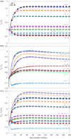 |
Fig. 1 Evolution of the solid (panel a), gas (panel b), and total torques (panel c) exerted on a 1 M⊕ planet over time (measured in terms of the number of orbits). The torques are normalized by the factor Γ0 = 2/q. The different models – with and without the back-reaction of the solid material – are represented by the empty and filled circles, respectively. The colors indicate the different types of solid material. |
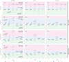 |
Fig. 2 Parameter study of the saturated torques felt by a low-mass planet in the range of 0.1 M⊕ ≤ Mp ≤ 10 M⊕. Panels A1–A3: solid torques in the BR models normalized by the absolute value of the solid torque in the corresponding NBR models. Panels B1–B3: gas torques in the BR models normalized by the absolute value of the gas torque in the NBR models. Panels C1–C3: total torques in the BR models normalized by the absolute value of the gas torque in the NBR models. Panels D1–D3: total torques in the NBR models normalized by the absolute value of the gas torque in the NBR models. The columns from left to right show three sets of models, each assuming a different steepness of the initial disk density profile, p = 0.5, 1.0, and 1.5. For each planet mass, three accretion efficiencies are examined: η = 0, 0.1, and 1. The colors indicate the different Stokes numbers (St = 0.01, 0.1, 1, 2, 3, 4, 5, and 10) used for the solid species in the parameter study. |
3.2 Parameter study on the effect of back-reaction
Figure 2 shows the normalized solid (A1, A2, A3), gas (B1, B2, B3), and total (C1, C2, C3) torques measured at the end of the simulations, after 200 orbits of the planet. Similar to Regály (2020), five different planet masses (0.1, 0.3, 1, 3.3, and 10 M⊕) with three different accretion efficiencies, η = 0, 0.1, and 1, were investigated. Simulations were performed with a different steepness of the disk surface mass density profile, assuming p = 0.5, 1.0, and 1.5. For comparison, the last row (D1, D2, D3) of Fig. 2 shows the total torques without the effect of back-reaction. In all cases, except for the solid torques in panels A1, A2, and A3, the torques were normalized by the absolute value of the gas torque measured in the NBR models,  . For the solid torques, the absolute value of the corresponding NBR solid torque,
  , was used as the normalization factor.
Based on the value of the normalized torques in the NBR case, three different regimes can be identified: a) ΓNBR/|ΓNBR| > 0, shaded with red; b) –1 < ΓNBR/|ΓNBR| < 0, shaded with blue; and c) ΓNBR/|ΓNBR| < –1, shaded with green colors. Torque measurements in the green or blue regions indicate that the disk exerts an increased or decreased amount of negative torque, respectively. Conversely, planets experience a positive torque from the disk if the measured torques are in the red region. Thus, at the boundary of the green and blue regions, the measured torques correspond to the canonical type I torques (Γ/Γ0 = –1).
Panels A1, A2, and A3 of Fig. 2 show the saturation values of the solid torques in the BR scenario, measured at the end of the simulation. In general, the back-reaction of the solid material has a marked effect on the solid torques for the coupled pebbles, St ≤ 0.1, for all the planet masses, accretion efficiencies, and initial density steepness investigated. Interestingly, there can be a torque reversal (where ΓBR/|ΓNBR| < 0) for the coupled species due to accretion and back-reaction. We also note that Mp = 10 M⊕ planets experience a significantly enhanced negative solid torque from the coupled species in BR models assuming p = 0.5. However, there is a weakened negative (for weak accretion, η ≤ 0.1) and positive (for strong accretion, η = 1) solid torque assuming p = 1 and 1.5. For the weakly coupled species, St ≥ 1, the solid torques are unaffected ( ) by the back-reaction of solid material felt by Mp ≥ 1 M⊕ planets. Conversely, for Mp ≤ 0.3 M⊕ planets, the back-reaction has a significant effect on the solid torques. We note that the effect of accretion efficiency can be clearly identified for the coupled species, St ≤ 0.1, while it is suppressed for St ≥ 1. It is noteworthy that for Earth-mass planets the solid torque of the species with St = 2 undergoes a sign change for p = 1 and 1.5 due to the back-reaction effect.
Panels B1–B3 of Fig. 2 show the gas torques for the three different steepnesses of the disk’s initial gas profile. Our results show that the effect of back-reaction significantly changes the gas torques for all planetary masses, accretion efficiencies, and initial density steepnesses studied. In BR models, the effect of accretion tends to weaken the magnitude of the gas torques exerted on Mp ≤ 1 M⊕ planets (i.e., the torques are in the blue regions). We note that the back-reaction of solid material has the most significant effect on the gas torques exerted on Earthmass planets. The strongest effect of accretion on the magnitude of the gas torque is found for Mp = 0.3M⊕ planets. In certain cases (St = 2 and 3, with p = 0.5), positive gas torques can be measured on Mp = 1 M⊕ as a consequence of the combined effect of back-reaction and high accretion efficiency. For Mp ≥ 3.3M⊕ planets, the effect of accretion on the gas torque is diminished. However, the effect of back-reaction tends to increase the magnitude of the negative gas torques for planets in this mass range.
The sum of the gas and solid torques – the total torques – are shown in panels C1–C3 of Fig. 2. In general, the back-reaction effect reduces the magnitude of the total negative torques exerted on Mp = 0.1–0.3 M⊕ planets compared to the NBR case. For Earth-mass planets, the influence of back-reaction increases the overall magnitude of the total torque when it is positive and decreases it when it is negative. However, this trend does not hold for species with St = 1; in this case, the negative torque is enhanced by back-reaction. We note that for shallow density profile disks, p = 0.5, a torque reversal occurs in BR models for Mp = 0.3 M⊕ planets accreting species of St = 5 with high efficiency and for Mp = 1 M⊕ planets interacting with St = 2 species regardless of accretion efficiency. We also find torque reversals in BR models for p = 1, St = 4 and 5, regardless of accretion efficiency and for St = 3 when η = 1. For p = 1.5, we no longer find positive total torques in the BR models (except for one model where St = 0.01 and η = 1), but the magnitudes of the negative total torques are significantly reduced compared to the NBR case. For larger planetary masses (Mp ≥ 3.3 M⊕), the influence of back-reaction reduces the magnitude of the total negative torques for almost all species (St < 10), regardless of accretion efficiency. However, for St = 10, the magnitude of the negative total negative torque is found to increase.
4 Discussion
4.1 Torque profiles in the vicinity of the planet
Here, we examine in detail the relationship between the measured torques and the torque profiles, as well as the density distributions around an Earth-mass planet, limiting our discussion to models with shallow initial density profiles of p = 0.5. However, the same analyses can be applied to simulations with p = 1 and p = 1.5.
To explain the results presented in Sect. 3, we first analyzed the radial torque profiles in the near-planetary regions. The azimuthally averaged torque profiles of solid species (Fig. A.1) and gas (Fig. B.1) in the vicinity of an Earth-mass planet as well as a detailed discussion can be found in the Appendices A–B. Our general observation is that the shape of the torque profiles is very similar for BR and NBR models. Although there is a little variation in the profile, the integrated torque values can be significantly different. It is noteworthy that the solid torques can only originate from the region of about ±3∆ RHill of the planet. In contrast, for the gas, this region extends to about ±15∆ RHill, regardless of whether the back-reaction is considered.
4.2 Distribution of gas and solid material around the planet
We shall now compare the distribution of solid and gaseous material surrounding an Earth-mass planet in the BR and NBR models. The plots illustrating the difference in solid (Figs. C.1–C.2) and gas (Figs. D.1–D.2) density distributions for the BR and NBR cases can be found in Appendices C–D.
The distribution of solid material changes significantly due to the combined effects of back-reaction and accretion (up to 60 percent density ratio for BR to NBR). An example is shown in Fig. 3 for an Earth-mass planet and St = 1 with p = 0.5. The effect of accretion as solid material becomes depleted close to the planet is clearly seen on the density distributions. A comparison of the density ratios in the BR and NBR models ( shown in the left panels of Fig. 3) shows that the effect of the back-reaction is to produce a density increase and decrease outside and inside the planetary orbit, respectively. As is shown in Figs. C.1 and C.2, a similar effect is observed for other Stokes numbers studied. Conversely, the change in the distribution of gas due to the back-reaction of solid material and accretion is less than 0.3%. Interestingly, the change in the distribution of solid material due to back-reaction does not significantly affect the magnitude of the solid torques (see Fig. A.1). However, it is clear that even small changes in the gas distribution can lead to a significant reduction in the magnitude of the gas torque exerted on the planet. To illustrate, the spiral waves generated by the gravitational influence of the planet are amplified in BR models for coupled pebbles with St ≤ 0.1. In contrast, for pebbles or boulders with stronger coupling (St ≥ 1), a significant depletion of gas is observed within the corotational region. Furthermore, the strength of the accretion serves to amplify the above phenomena.
Due to the low viscosity values used, planets with 10 M⊕ reach the isolation mass, as is shown in Ataiee et al. (2018). As a result, a weak (few-percent density depletion) partial gap is opened in the gas disk. The pressure maxima developed at the edges of the gap effectively collect solid material, especially for St = 1. An example of the solid material distribution as well as the azimuthally averaged radial density profiles for St = 1 and η = 0 are shown in Fig. 4. However, as we have shown (see e.g. Fig. A.1 for details), no significant torque is exerted by the solid material beyond the region ΔR > 3 RHill. We note that in the long-term (several hundred thousand orbits) evolution of planet-disk interaction models, the corotation region can be emptied by the combined effect of solid material accretion and the pressure trap. As a result, the solid torque can be reduced, but it is already negligible for 10 M⊕ planets.
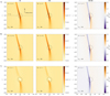 |
Fig. 3 Distribution of St = 1 solid material in the vicinity of an 1 M⊙ planet in BR and NBR models assuming η = 0 (panels A), η = 0.1 (panels B), and η = 1 (panels C) with p = 0.5. The density ratio of the BR and NBR models are also shown on the left. The circles represent the planetary Hill sphere. The axes are shown in code units. |
4.3 Caveats of our models
Finally, we discuss the caveats to our simulations that will be addressed in future research. First, we modeled the planet-disk interaction in two dimensions for the case in which one has to smooth the gravitational potential of the planet defined by Eq. (6). The smoothing length was chosen to be ϵ = 0.6 for both gas and solid material. We note that the vertical scale height of the solid material may differ from that of the gas due to the size-dependent rate of sedimentation to the disk midplane (Dullemond & Dominik 2004). However, using a planetary potential that depends on the Stokes number of solid material has no firm basis and requires further three-dimensional investigations. Thus, both solid material and gas experience the same smoothing of the planetary potential in our simulations. Rendon Restrepo & Barge (2023) provided an analytical expression for the spatially varying smoothing length for twodimensional protoplanetary disk simulations in which both dust and gas self-gravity are calculated. As we showed in Regály (2020), more or less smoothing reduces or increases the density asymmetry around the planet. Recently, Chrenko et al. (2024) studied the effect on the solid torques exerted by pebbleaccreting low-mass planets, using Lagrangian superparticles to represent the pebbles. In their model, therefore, no smoothing of the gravitational potential for pebbles is necessary. Although they neglect the back-reaction of solid material, their results also show a positive total torque for Mp ≤ 3 M⊕ planets for a range of Stokes numbers, 0.01 ≤ St ≤ 0.785.
We note, however, that three-dimensional models are necessary to model planetary accretion, which is a three-dimensional phenomenon in reality. It has been shown that millimeter-sized dust in the circumplanetary region of a forming giant planet does not settle in the disk midplane (Szulágyi et al. 2014; Fung et al. 2015; Szulágyi et al. 2022; Cilibrasi et al. 2023; Maeda et al. 2024). As a result, the pebbles are delivered to the circumplanetary region by the meridional circulation accreted from the vertical direction, flowing together with the gas. Since this vertical mixing of the spiral waves can modify the two-dimensional angular momentum loss three-dimensional simulations should also be considered for low-mass planets in the future. Fung et al. (2015) have also reported a migration rate of a 5 M⊕ planet that is a factor of three slower due to three-dimensional effects, but this can be suppressed by a sufficiently large disk viscosity, leading to results similar to two-dimensional simulations.
It is known that relatively large particles with Stokes numbers well above unity can cross each other’s orbit. In this case, the fluid approach used in this study may neglect some aspects of orbital dynamics. In light of the above considerations, it would be preferable to use a comparable Lagrangian approach, as is used in Chrenko et al. (2024), instead of our current simplified methodology for modeling accretion phenomena. In this case, however, the diffusion of particles requires a particlebased implementation of diffusion, similar to the method used in Picogna et al. (2018). This will be left to a future study.
The effect of thermodynamics is also neglected in our study because we used a locally isothermal approximation. Since pebble accretion can transport significant energy to the planet, the heating of the circumplanetary material is inevitable. As a result, a significant temperature contrast develops around the planet, which can eventually cause torque reversal (Paardekooper & Mellema 2006; Benítez-Llambay et al. 2015). Two-dimensional hydrodynamic simulations by Kley & Crida (2008) have already shown that low-mass planets (Mp ≤ 50 M⊕) migrate outward in radiative disks at a rate comparable to that of standard type I migration. This torque reversal has also been confirmed for planets in the range of 2–5 M⊕ in three-dimensional hydrodynamic models (Kley et al. 2009; Lega et al. 2014). Thus, it is necessary to include the thermodynamic effects of solid accretion in future investigations.
We neglected the effect of the disk’s own gravity by assuming that the disk mass is small. However, in a more massive disk the results may differ from ours. For example, Crida et al. (2009) showed that neglecting the self-gravity of the disk requires careful handling of the material in the planet’s Hill sphere. In our simulations, we did not apply a torque cutoff inside the Hill sphere. This assumption is plausible, since the circumplanetary disk does not form around low-mass, Mp ≲ 30 M⊕, planets (Masset et al. 2006). Thus, the exclusion of material in the planetary Hill sphere has no physical argument. We emphasize that Baruteau & Masset (2008) showed that the disk self-gravity is slightly accelerating type I migration. It should be noted that we have used arithmetically distributed radial grid cells, while the calculation of the self-gravity of the disk by fast Fourier algorithms (see, e.g., Vorobyov & Basu 2010, 2015; Regály & Vorobyov 2017b) requires logarithmically distributed radial grid cells.
We utilized a low-viscosity approach that deserves further investigation at higher viscosities. The rationale behind this assertion is that in this particular scenario, the diffusion of solid material will be more pronounced, since diffusion is directly proportional to viscosity (Eq. (13)). As a result, the asymmetry observed around the planet may be less pronounced, which could weaken the effect of the back-reaction of solid material. However, it should be noted that for larger Stokes numbers, diffusion will have a less significant effect, since the diffusion coefficient is inversely proportional to the square of the Stokes number.
Furthermore, the analysis given in this paper considers only the accretion of solid material, while the accretion of gas is neglected. In addition, the mass of solid material accreted by the planet is also not included in the planetary mass. However, this may be a plausible assumption for low-mass planets, since we modeled the planet-disk interaction for only 200 orbits, which limits the amount of material accreted onto the planet.
The low-mass planet was fixed in a circular orbit in our simulations; that is, no migration was allowed. Guilera et al. (2023) calculated the formation tracks of low-mass embryos using the torque measurements of Benítez-Llambay & Pessah (2018). They found that low-mass planets (≤10 M⊕) migrate outward beyond the water-ice line for St = 0.1 and provide the seed for massive planets. It is therefore also worth investigating the effect of the back-reaction of the solid material combined with solid accretion in models in which planets are free to migrate.
Our models use a fixed Stokes number approximation for the solid species rather than a given size distribution for the solid material. In the latter case, the Stokes number increases with stellar distance (Weidenschilling 1977). We note, however, that the radial range around the planet from which the solid torque is exerted is relatively small, only a few times the size of the planetary Hill sphere. Nevertheless, it is desirable to calculate the local Stokes number based on the particle size when modeling evolutionary tracks.
Varying the metallicity (the dust content of the disk) can change our results, since the higher the metallicity, the higher the dust content of the disk. For example Hsieh & Lin (2020) found stochastic migration of 2 M⊕ planets for high metallicity (Z > 0.3) and St ≳ 0.03; that is, for higher dust content than in our model. It is therefore worth investigating the effect of disk metallicity on planetary torques in models that take into account the back-reaction of solid material.
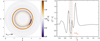 |
Fig. 4 The normalized density distribution of the St=1 solid material after 200 orbits of a 10 M⊕ planet, assuming η = 0. Left: two dimensional distribution. Right: azimuthally averaged radial density profile of solid material. The inner and outer Hill radii are represented by dashed black lines. |
5 Conclusions
We have studied how the back-reaction of solid material affects the solid, gas, and total torques exerted on low–mass (0.1–10 M⊕), solid-only accreting planets. To achieve this, we performed two-dimensional hydrodynamic simulations that model the interaction between the accreting planet and the disk using the code GFARGO2. We treated the solid material as a pressureless fluid and the disk was assumed to be locally isothermal. The solid components of the disk were assumed to have fixed Stokes numbers in the range of 0.01 ≤ St ≤ 10. Diffusion of the solid material was also taken into account. Simulations for different planetary masses and accretion efficiencies were performed with (BR models) and without (NBR models) the effect of the back-reaction of solid material. The saturation value of the torque experienced by a non-migrating planet was determined after 200 orbits. Our findings can be summarized as follows:
In general, the magnitude of the solid torques is only slightly affected by the back-reaction. The magnitude of the solid torque is observed to decrease in cases in which planets are accreting, with the potential for torque reversal to occur for those species that are still coupled to the gas, St ≤ 0.1. These phenomena are independent of the steepness of disk density profile;
In general, the gas torques are negative and show an increase in magnitude for all planetary masses studied under investigation in non-accreting models. It is noteworthy that Earthmass planets show a distinctive behavior, with gas torques measured as being significantly weakened for St ≥ 2. The back-reaction effect increases with the accretion efficiency and decreases with the steepness of the disk density profile;
In general, the magnitude of the total torque is increased by the effect of back-reaction, regardless of its sign. However, the combined effect of planetary accretion and back-reaction tends to reduce of the magnitude of negative torques;
Compared to the canonical type I prediction, Mars-sized or slightly larger planets (Mp = 0.1–0.3 M⊕) with high accretion efficiency experience a weakened magnitude torque or even a torque reversal for coupled pebble-sized solid material (St ≤ 0.1). However, an increased magnitude of negative torque is measured for less coupled solid components (St ≥ 0.1). The steepness of the disk density profile has no significant effect on the above phenomena;
Earth-mass planets also experience a weakened magnitude of negative torque from the disk containing pebble-sized solid species (St ≤ 0.1). However, the effect of back-reacting boulders (St = 3–5) is to strengthen the positive torque (or weaken the negative torque for steep disk density profiles), which requires a shallow disk density profile. Conversely, the negative torques are strengthened for St = 1 or St = 10;
Super Earths (Mp ≥ 3.3 M⊕) never experience positive total torques. The magnitudes of the total torques are still weakened compared to the type I prediction, however, but the effect of the back-reaction of the solid material mitigates the discrepancy. The accretion efficiency has no significant effect on the total torque.
As is shown, the back-reaction of the solid material has the effect of reducing the magnitude of the negative torques exerted on the planets, while at the same time increasing the magnitude of the positive torques exerted on the planets. This phenomenon is most pronounced in the case of Earth-mass planets. Assuming that our torque measurements are applicable to planets whose orbits are not fixed and that the pressureless fluid approximation of solid material is valid, the following train of thought can be advanced.
Mars-sized planetary embryos that accrete pebbles with high efficiency can migrate outward during their nascent phase when the solid material is still coupled to the gas of the protoplanetary disk. Should the size of the solid components reach the size of boulders during this initial stage of planet formation, the planetary embryos will undergo a relatively rapid inward migration. We note, however, that the rate of migration of these small embryos at this stage of evolution is quite slow. Planets that reach a mass comparable to that of Earth are subject to outward migration due to the influence of solid material in the boulder regime. Once a planet’s mass exceeds that of the Earth, the direction of migration is reversed again, with a reduced rate compared to that predicted by the type I regime.
It should be emphasized that the deviation from the migration history predicted by the canonical type I theory may be more pronounced in disks with a higher metal content. Furthermore, it is predicted that the negative total torques, which have been reduced in magnitude as a result of the back-reaction of solid material, can be further weakened and may become positive if the metal content of the disk is sufficiently high. In light of the above findings, we conclude that planetary system formation may benefit from the combined effect of back-reaction and accretion by reducing the risk of young planets being engulfed by the central star.
Acknowledgements
ZsS acknowledges the support of the NKFIH excellence grant TKP2021-NKTA-64.
Appendix A Solid torque profiles for a 1 M⊕ planet
This section presents a detailed analysis of the solid and gas torque profiles in the vicinity of an Earth-mass planet, assuming p = 0.5 and η = 0, 0.1 and 1. The azimuthally averaged radial torque profile, Γi, is calculated as
 (A.1)
(A.1)
where Γi,j /Γ0 is the torque originating from cell i, j. Figure A.1 shows the azimuthally averaged solid torque profiles exerted by eight different types of of solids. The colors indicate the two different types of models: those with (purple) and those without the back-reaction of solid material (green), respectively. The difference in the measured torques between the two models,  , is shown in red bellow each panel. The sum of the BR and NBR torques along the X-axis is shown in the figures as purple and green numbers, respectively. The modeldependent solid torque ratio in percent (hereafter referred to as solid torque ratio henceforth),
  , is shown in red on each panel. Note, that the values displayed on the vertical axis are multiplied by a factor of 103 for the sake of clarity. The horizontal axis shows the relative distance from the planet, expressed in units of the planet’s Hill radius. It is also important to note, that in the case of solid torque profiles, we only show the region close to the planet (±3 ΔRHill). This is because the solid torque is only significant up to this distance and generally disappears beyond ±6 ΔRHill (Regály 2020).
First, we examined the torque profiles of the solid material assuming η = 0 and p = 0.5 (left column of Fig. A.1). The shape of the solid torque profiles are the same for the NBR and BR cases for all investigated species. The torques of the coupled solid species (St < 0.1) show small discrepancies (less than 1 percent) in the torque amplitude between the BR and NBR scenarios. While the change in the torque amplitude can reach up to about 207 percent for species with St = 0.1, the solid torque amplitudes for the coupled species are so small (less than 1e-2), that this difference will not have a meaningful effect on the solid torque exerted on the planet. This explains why the solid torques seen in our models (panel a of Fig. 1) are the same for these species.
For St = 1, the torque profile is shifted downward when the back-reaction is taken into account and the solid torque is about 146 percent that of observed in the NBR case. As a result, the planet experiences an increase in the magnitude of the negative torque of this type (light blue curve in panel b of Fig. 1).
For St = 2, the back-reaction causes the left wing of the positive peak and the negative peak of the solid torque to shift upward, resulting in a torque ratio of about 124 percent. As a result, the planet experiences an increase in the magnitude of the positive solid torque in the BR case (purple curve in panel a of Fig. 1).
For species with St = 3-5, the torque amplitude decreases in the range [−1ΔRHill, + 1ΔRHill], while it increases outside this range. For these weakly coupled species, the influence of the back-reaction is less pronounced, the torque ratio is only about 96–98%. This explains the slightly lower saturation values for the BR torques of these species seen in panel a of Fig. 1. For species with St = 10, the change in torque magnitude is the smallest, about 94 percent of that observed in the NBR case (dark red curve on panel a of Fig. 1).
Next we examined the effect of accretion on the solid torque profiles (middle and right columns of Fig. A.1). In general, the effect of accretion has no significant impact on the shape of the radial solid torque profiles.
Weak accretion (η = 0.1) of species with St ≤ 0.1 increases the torque amplitude inside the Hill sphere in the BR case if the sign of the torque is positive (St = 0.01) and decreases if it is negative (St = 0.1). As a result both the positive and negative solid torques are weakened compared to the NBR case. Strong accretion (η = 1) of these species reduces the magnitude of the solid torques in the BR case.
For species with St = 1, the difference in the torque magnitude decreases as the accretion efficiency increases. This results in a the decrease in the solid torque ratio to about 125 and 96 percent for η = 0.1 and 1, respectively.
For species with St = 2, the torque magnitude is observed to increase to 133 percent of that in the NBR case when η = 0.1, but only up to about 117 percent when the planet is heavily accreting (η = 1) this solid material. For species with St = 3–10, the change in the torque ratio is negligible, showing a variation of only about 1 percent between the two different accretion scenarios.
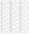 |
Fig. A.1 Comparison of solid torque profiles for 1 M⊕ planet, assuming p = 0.5 and η = 0, 0.1 and 1 in BR and NBR models. Note that the values shown on the vertical axis are multiplied by a factor of 103 for the sake of clarity. |
Appendix B Gas torque profiles for a 1 M⊕ planet
Figure B.1 shows the azimuthally averaged radial gas torque profiles caused by the interaction with different species (St = 0.01, 0.1, 1, 2, 3, 4, 5, and 10) of solid material in the vicinity of 1 M⊕ planet, assuming p = 0.5 and η = 0, 0.1, and 1. Compared to the solid material, the radial torque of the gaseous component can reach or even exceed, ±10 ΔRHill (Regály 2020). Therefore, a larger area must be displayed in order to study its variation (±15 ΔRHill in our case). The colors indicate the two types of models, with (purple) and without (green) the back-reaction of the solid material, respectively. The difference between the two models,  , is shown in red below each panel. The total BR and NBR torques along the X-axis and the sum of their difference are shown as purple, green and red numbers, respectively. The model-dependent ratio of the torques in percent (hereafter referred to as the gas torque ratio),
  , is represented by the red numbers in each panel. Note that, as in the previous case, the values on the vertical axis are multiplied by 103 for the sake of clarity. The relative distance from the planet is given in units of the planet’s Hill radius.
Next we examined the torque profiles assuming η = 0 and p = 0.5 (left column of Fig. B.1). Similar to solids, the shape of the gas torque profiles is also independent of whether the BR or NBR case is being considered. For species with St ≤ 1, the sign of the gas torques remains negative and the gas torque ratio increases with the Stokes number, reaching a value of about 164 percent.
The back-reaction of species with St = 1 causes the gas torque amplitude to decrease in the range [−3ΔRHill, +8ΔRHill]. This explains the increase in the saturation value of the negative gas torque shown in panel b of Fig. 1 for this solid species. However, for the weakly coupled species (St = 2–10), the gas torque amplitude is increased between ±5 ΔRHill in the BR case. As a result, the gas torque ratio decreases significantly, and reaches a minimum value of about 8 percent that in the NBR case, when St = 2 and 3. This explains the significantly reduced negative saturation values in the BR case for these species (purple, green, yellow, blue and brown curves of panel b in Fig. 1). In contrast to the solid torque profiles, the change in the torque magnitude for these species decreases with Stokes number.
The middle and right columns of Fig. B.1 show the azimuthally averaged radial gas torque profiles in two different accretion regimes (η = 0.1 and 1, respectively). It is noteworthy that in the case of the coupled species, solid accretion leads to a reduction in the magnitude of the negative gas torque. For St = 0.01 and 0.1, the torque magnitude in the weakly accreting scenario (η = 0.1) is about 89 percent that of the NBR case. Furthermore, in the strongly accreting scenario (η = 1), the gas torque ratio is significantly reduced by the accretion of these species, down to about 42 and 23 percent, respectively. For species with St = 1, the torque ratio between BR and NBR cases decreases as the efficiency of solid accretion increases.
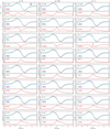 |
Fig. B.1 Comparison of gas torque profiles for 1 M⊕ planet, assuming p = 0.5 and η = 0, 0.1 and 1. in BR and NBR models. Note, that the shown values on the vertical axis are multiplied by a factor of 103 for the sake of clarity. |
In contrast to solids, the amplitude of the torque exerted by the gaseous component increases between ±5 RHill in the weakly and strongly accreting scenarios, when interacting with species with St = 2–10. As a result, the magnitude of the gas torque for these species continues to decrease compared to the NBR case.
For species with St = 2, the magnitude of the negative gas torque is further reduced by accretion and undergoes a change in sign, reaching a magnitude of about 0.25 percent that of the NBR case when η = 0.1.
For St = 3, the gas torque is also positive in the BR case when η = 1, with a gas torque ratio of about 10 percent. It is significant that the gas torque becomes positive in these cases (see the purple and dark green symbols in panel B1 of Fig. 2). For species with St = 4 and 5, the influence of back-reaction and accretion does not lead to torque reversal, but the negative torques are significantly reduced compared to the NBR case. Similar to the non-accreting scenario (η = 0), the change in the gas torque magnitude (i.e., the gas torque ratio) is observed to decrease with Stokes number for these species. For species with St = 10, the gas torque ratio increases slightly with the accretion efficiency to about 79 percent when η = 1.
Appendix C Spatial distribution of solid material around an Earth-mass planet
Figures C.1 and C.2 show the ratio of the NBR to BR solid surface density distribution in the vicinity of a 1M⊕ planet, assuming p = 0.5 and three different accretion strengths. The density distributions are shown in a co-moving frame of the planet. The material situated in the region in front (Y > 0) or behind (Y < 0) the planet (with respect to the orbital motion) exerts a positive or negative torque, respectively. The rows represent the different types of solid species studied (St = 0.01, 0.1, 1, 2, 3, 4, 5, and 10), while the columns indicate increasing accretion efficiency (η = 0, 0.1, and 1). The comparison is calculated as  . Note that the axis values are displayed in code units.
We first considered models with η = 0 (left column of Fig. C.1). Due to the remarkably low comparison values observed for species with St = 0.01, and 0.1, the values shown in the figures have been multiplied by 250 and 25, respectively. For St = 0.01, even after multiplying the values, the change in the distribution between the BR and BR cases is very small. Since this change is symmetrical to the Y = 0 axis, the torques remain unchanged between the BR and NBR cases (St = 0.01, η = 0 panel of Fig. A.1). For St = 0.1, the density of the solid material is reduced in the inner part of the corotation region in the BR model. Conversely, a slight increase in the density of solid material is observed at the outer side of the corotation region, behind the planet. Consequently, the distribution of solid material along the Y = 0 axis will be asymmetric, resulting in a BR to NBR torque ratio of about 207 percent (St = 0.1, η = 0 panel of Fig. A.1). This phenomenon is more pronounced for species with St = 1, which explains the measured torque ratio of about 146 percent and a negative torque that is increased in magnitude in the BR case (St = 1, η = 0 panel of Fig. A.1).
For St = 2, the disk is significantly reduced in solid material in the region behind the planet in the BR model. This asymmetry along the Y = 0 explains an explanation for the observed change in the torque ratio and the increase in the magnitude of the solid torque in the BR case.
For species with St = 3, the region behind the planet in solid material is still reduced compared to the NBR case, but this reduction is less pronounced than in the case of St = 2 (Fig. C.2). For species with St = 4 and 5, the empty region behind the planet starts to decrease in the BR model. Furthermore, in the region inside the planetary orbit, there is an enhancement of solid material develops in the BR case. This results in an increased contribution of negative solid torque from the inner disk, which ultimately leads to a decrease in the magnitude of the solid torque compared to the NBR case. The distribution of solid material becomes increasingly asymmetric with respect to the Y = 0 axis as the Stokes number increases. This phenomenon is reflected in the weakening of the solid torque magnitudes for these species (St = 3-5, η = 0 panel of Fig. A.1).
However, for species with St = 10, there is a slight decrease in the density of the solid material behind the planet and outside the planetary orbit in the BR case. Note, that here the density values are multiplied by 25 for clarity. Consequently, the magnitude of the negative torque decreases in the BR case (St = 10, η = 0 panel of Fig. A.1).
Regály (2020) showed that the accretion of solid material changes its distribution around the planet and thus the magnitude of the solid torque exerted on the planet. Let’s now compare the distribution of solid material in the BR and NBR cases in two accretion regimes, η = 0.1 and 1 (middle and right columns of Figs. C.1-C.2). Note that for species with St = 0.01 and 0.1, the density values on the figures are multiplied by 25 for η = 0.1. As the accretion efficiency increases the density of solid material inside the corotation region decreases slightly, while outside it increases for St = 0.01. This increasing asymmetry in the solid material explains the measured 84 percent torque ratio between the BR and NBR cases. The largest asymmetry is seen for η = 1. For St = 0.1, the combined effect of back-reaction and high accretion efficiency (η = 1) results in an increased density of solid material in the corotation region in the BR models. However, the aforementioned discrepancy will only result in a torque ratio of about 98 percent, provided that the change in the distribution of solid material remains symmetric with respect to the Y = 0 axis of the planet (St = 0.1, η = 1 panel of Fig. A.1).
For St = 1, as the accretion efficiency increases, the density asymmetry of the sold material at the inner and outer corotation regions weakens. Consequently, the change in the distribution of solid material becomes increasingly symmetric with respect to the Y = 0 axis, resulting in a reduction of the torque ratio to about 96 percent when η = 1 (St = 1, η = 1 panel of Fig. A.1).
For species with St = 2, the density of solid material at the outer part of the corotation region increases when η = 1. Consequently, in the BR case, the region situated behind the planet exerts a greater influence on the solid torque, leading to a reduction of the torque ratio to about 117 percent (St = 2, η = 1 panel of Fig. A.1).
For St = 3, the density of solid material at the outer part of the corotation region increases with the accretion efficiency. However, for η = 1 this change in distribution only results in a torque ratio of 97 percent.
For St = 4 and 5 both the density enhancement (Λ-shape pattern) and depression (pattern behind the planet) increase with accretion efficiency. As a result, the magnitudes of the solid torque vary only slightly in the BR models. Since the above phenomenon weakens with Stokes number, it is evident that the effect of accretion on the torque ratio diminishes with increasing Stokes number for the boulder-sized solid species.
For St = 10, the region around the planet is emptied with increasing accretion efficiency. However, the torque ratio decreases by only about 1 percent from η = 0 to η = 1 (St = 10 panels of Fig. A.1).
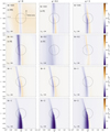 |
Fig. C.1 Comparison of solid density distributions in NBR and BR models for St = 0.01, 0.1, 1, and 2, with three different accretion efficiencies (η = 0, 0.1, and 1), in the vicinity of 1 M⊕ planet. The axes are shown in code units. Colors ranging from dark purple to brown represent increasing solid densities in the BR models. Regions where the two models are the same are shown in white. The black circle indicates the planetary Hill sphere. |
Appendix D Spatial distribution of gas around an Earth-mass planet
Figures D.1 and D.2 illustrate the comparison of the gas density distribution of NBR and BR models, with three different efficiencies of solid accretion, around 1 M⊕ planet in the p = 0.5 disk. The comparison is calculated as  .
.
The colors ranging from blue to red represent increasing gas densities in BR models. Regions where the two models agree are shown in white. The density distributions are shown in a comoving frame of the planet. Note that the values shown in the figures are multiplied by a factor of 103 for the sake of clarity.
First, we examined the cases where η = 0 (left column of Figs. D.1 and D.2). In the case of the coupled pebble-sized species (St = 0.01), an increase in gas density is observed in the BR model within the region where spiral waves have formed as a result of the gravitational interaction between the planet and the disk. In addition, a decrease in gas density is observed both the inside and outside the inner and outer spiral waves, respectively. These variations in the distribution only result in a BR to NBR torque ratio of about 99 percent, due to the fact that the variation is symmetric to the Y = 0 axis (St = 0.01, η = 0 panel of Fig. B.1). A similar pattern is observed for St = 0.1. However, the corotation region ahead of the planet shows a slight decrease in the gas in the BR model. As a result, the torque ratio increases, and the planet experiences an increased magnitude of negative torque from the gas (St = 0.1, η = 0 panel of Fig. B.1).
For species with St = 1, the back-reaction also causes enhanced spiral waves in the gas similar to the coupled species. However, the gas in the corotation region shows a more pronounced depletion, especially in the region in front of the planet.
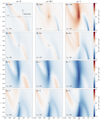 |
Fig. D.1 Comparison of gas density distributions in NBR and BR models for St = 0.01, 0.1, 1, and 2, with three different accretion efficiencies (η = 0, 0.1, and 1), in the vicinity of 1 M⊕ planet. The axes are shown in code units. Colors ranging from blue to red represent increasing gas densities in the BR models. Regions where the two models agree are show in white. The black circle indicates the planetary Hill sphere. Note that the density ratios are multiplied by 1000 for clarity. |
As a result, the regions in front the planet contribute less to the torque exerted on the planet in the BR case. This explains the observed BR to NBR torque ratio and the increase in the magnitude of the negative torque (St = 1, η = 0 panel of Fig. B.1).
For St = 2, the back-reaction effect leads to a decrease of the gas density in the corotation region behind the planet, compared to the NBR case. In addition, the density of the gas within the planetary orbit and in front of the planet, also increases. Therefore, the contribution to the gas torque from the inner and outer regions is larger and smaller, respectively, in the BR case. This results in a torque ratio of about 8 percent and a significant reduction in the magnitude of the negative gas torque (St = 2, η = 0 panel of Fig. B.1).
In the BR case, for species with St = 3 (St = 3, η = 0 panel of Fig. D.2), the gaseous material inside the planetary orbit increases while the material outside the orbit decreases. Thus, the effect of the back-reaction of this species leads to a markedly asymmetric distribution of the gas with respect to the Y = 0 axis, thereby generating a significant weakening of the magnitude of the negative gas torque in the BR case (St = 3, η = 0 panel of Fig. B.1). For St = 4–5, a similar pattern appears. The accumulation of gaseous material inside and outside the planetary orbit is observed to increase with the Stokes number. Consequently, the BR to NBR torque ratio and the magnitude of the negative torque are observed to increase in the BR case when compared to species with St = 2–3. Nevertheless, the reduction in torque magnitude in BR models remains significant compared to the NBR case (St = 4–5, η = 0 panels of Fig. B.1).
In the BR model, for species with St = 10, there is a slight decrease and increase in the density of the gas density present inside and outside the planetary orbit, respectively. Therefore, the region in front of the planet has a slightly larger effect on the gas torque in the BR case, while the regions beyond the planet have a smaller effect. As a result, the magnitude of the negative torque is reduced in the BR case (St = 10, η = 0 panel of Fig. B.1).
The middle and right columns of Figs. D.1-D.2 show the comparison of the gas density distribution in two different accretion regimes, η = 0.1 and 1, respectively. For St = 0.01, as the accretion efficiency increases, the amount of gas in the corotation region in front of the planet also increases. Conversely, the density of gas present in the spiral waves is observed to decrease compared to the NBR case. Thus, the region in front of the planet contributes more to the gas torque exerted on the planet. As a result, the magnitude of the negative torque decreases with accretion efficiency. For St = 0.1, the region in front of the planet is no longer reduced in gaseous material compared to the NBR case for η = 0.1. As a consequence, the magnitude of the gas torque is observed to decrease in the BR case, resulting in a BR-to-NBR torque ratio of about 89 percent (St = 0.1, η = 0.1 panel of Fig. B.1). Moreover, in the BR case, high accretion efficiency leads to an increase and a decrease in the density of the gas inside and outside the orbit of the planet, respectively. The aforementioned variation in the distribution leads to a noticeable reduction in the magnitude of the negative gas torque in the BR case (St = 0.1, η = 1 panel of Fig. B.1).
The back-reaction of species with St = 1 causes the difference in gas distribution of the spiral waves to decrease with increasing accretion efficiency. In addition, the gas density within the corotation region continues to decrease and extends the region behind the planet for η = 0.1 and 1. As a result, the magnitude of the gas torque shows a slight decrease with increasing accretion efficiency (St = 1, η = 0.1 and 1 panels of Fig. B.1).
For St = 2, the density in the spiral waves behind the planet decreases as the accretion efficiency increases. Moreover, the amount of gas inside the planetary orbit increases compared to the NBR case. As a result, the BR-to-NBR torque ratio decreases significantly and even changes sign when η = 0.1. For η = 1, the torque ratio and the magnitude of the positive gas torque increase due to solid accretion (St = 2 panels of Fig. B.1).
For species St = 3–5, solid accretion slightly decreases and increases the amount of gas inside and outside the planetary orbit, respectively. As a result, the spiral waves preceding and following the planet will have more positive and less negative contributions to the gas torque in the BR case, respectively. This leads to a further weakening of the torque ratio between the BR and NBR cases. Note that for St = 3 the gas torque also changes sign when η = 1 (St = 3–5, η = 0.1, and 1 panels of Fig. B.1). Thus, the gas distribution becomes increasingly asymmetric with respect to the Y = 0 axis, which also leads to an increase of the BR to NBR torque ratio for these species (St = 3–5, η = 0.1 and 1 panels of Fig. B.1). However, the increase in the torque difference is also observed to decrease with the Stokes number, analogous to the η = 0 scenario.
For St = 10, the accretion of solid material leads to a slight depletion of gas near the planetary orbit in the BR case. However, these changes result in only a small increase in the torque ratio and the magnitude of the negative gas torque does not change significantly (St = 10, η = 0.1 and 1 panels of Fig. B.1).
References
- Ataiee, S., Baruteau, C., Alibert, Y., & Benz, W. 2018, A&A, 615, A110 [NASA ADS] [CrossRef] [EDP Sciences] [Google Scholar]
- Baruteau, C., & Masset, F. 2008, ApJ, 678, 483 [NASA ADS] [CrossRef] [Google Scholar]
- Benítez-Llambay, P., & Pessah, M. E. 2018, ApJ, 855, L28 [Google Scholar]
- Benítez-Llambay, P., Masset, F., Koenigsberger, G., & Szulágyi, J. 2015, Nature, 520, 63 [Google Scholar]
- Chrenko, O., Chametla, R. O., Masset, F. S., Baruteau, C., & Brož, M. 2024, A&A, 690, A41 [NASA ADS] [CrossRef] [EDP Sciences] [Google Scholar]
- Cilibrasi, M., Flock, M., & Szulágyi, J. 2023, MNRAS, 523, 2039 [CrossRef] [Google Scholar]
- Crida, A., Baruteau, C., Kley, W., & Masset, F. 2009, A&A, 502, 679 [NASA ADS] [CrossRef] [EDP Sciences] [Google Scholar]
- de Val-Borro, M., Edgar, R. G., Artymowicz, P., et al. 2006, MNRAS, 370, 529 [Google Scholar]
- Dipierro, G., Laibe, G., Alexander, R., & Hutchison, M. 2018, MNRAS, 479, 4187 [NASA ADS] [CrossRef] [Google Scholar]
- Dullemond, C. P., & Dominik, C. 2004, A&A, 421, 1075 [NASA ADS] [CrossRef] [EDP Sciences] [Google Scholar]
- Fung, J., Artymowicz, P., & Wu, Y. 2015, ApJ, 811, 101 [Google Scholar]
- Gárate, M., Birnstiel, T., Stammler, S. M., & Günther, H. M. 2019, ApJ, 871, 53 [CrossRef] [Google Scholar]
- Gárate, M., Birnstiel, T., Drazkowska, J., & Stammler, S. M. 2020, A&A, 635, A149 [NASA ADS] [CrossRef] [EDP Sciences] [Google Scholar]
- Gonzalez, J. F., Laibe, G., & Maddison, S. T. 2017, MNRAS, 467, 1984 [NASA ADS] [Google Scholar]
- Gonzalez, J. F., Laibe, G., & Maddison, S. T. 2018, in SF2A-2018: Proceedings of the Annual meeting of the French Society of Astronomy and Astrophysics, eds. P. Di Matteo, F. Billebaud, F. Herpin, et al. [Google Scholar]
- Guilera, O. M., & Sándor, Z. 2017, A&A, 604, A10 [Google Scholar]
- Guilera, O. M., Benitez-Llambay, P., Miller Bertolami, M. M., & Pessah, M. E. 2023, ApJ, 953, 97 [NASA ADS] [CrossRef] [Google Scholar]
- Hsieh, H.-F., & Lin, M.-K. 2020, MNRAS, 497, 2425 [NASA ADS] [CrossRef] [Google Scholar]
- Kanagawa, K. D., Ueda, T., Muto, T., & Okuzumi, S. 2017, ApJ, 844, 142 [NASA ADS] [CrossRef] [Google Scholar]
- Kley, W., & Crida, A. 2008, A&A, 487, L9 [NASA ADS] [CrossRef] [EDP Sciences] [Google Scholar]
- Kley, W., Bitsch, B., & Klahr, H. 2009, A&A, 506, 971 [NASA ADS] [CrossRef] [EDP Sciences] [Google Scholar]
- Kley, W., Müller, T. W. A., Kolb, S. M., Benítez-Llambay, P., & Masset, F. 2012, A&A, 546, A99 [NASA ADS] [CrossRef] [EDP Sciences] [Google Scholar]
- Lega, E., Crida, A., Bitsch, B., & Morbidelli, A. 2014, MNRAS, 440, 683 [Google Scholar]
- Lyra, W., Johansen, A., Klahr, H., & Piskunov, N. 2008, A&A, 491, L41 [NASA ADS] [CrossRef] [EDP Sciences] [Google Scholar]
- Lyra, W., Paardekooper, S.-J., & Mac Low, M.-M. 2010, ApJ, 715, L68 [Google Scholar]
- Maeda, N., Ohtsuki, K., Suetsugu, R., et al. 2024, ApJ, 968, 62 [NASA ADS] [CrossRef] [Google Scholar]
- Masset, F. S. 2000, in Disks, Planetesimals, and Planets, eds. G. Garzón, C. Eiroa, D. de Winter, & T. J. Mahoney, Astronomical Society of the Pacific Conference Series, 219, 75 [NASA ADS] [Google Scholar]
- Masset, F. S. 2002, A&A, 387, 605 [NASA ADS] [CrossRef] [EDP Sciences] [Google Scholar]
- Masset, F. S., Morbidelli, A., Crida, A., & Ferreira, J. 2006, ApJ, 642, 478 [Google Scholar]
- Müller, T. W. A., Kley, W., & Meru, F. 2012, A&A, 541, A123 [NASA ADS] [CrossRef] [EDP Sciences] [Google Scholar]
- Nakagawa, Y., Sekiya, M., & Hayashi, C. 1986, Icarus, 67, 375 [Google Scholar]
- Paardekooper, S. J., & Mellema, G. 2006, A&A, 459, L17 [CrossRef] [EDP Sciences] [Google Scholar]
- Picogna, G., Stoll, M. H. R., & Kley, W. 2018, A&A, 616, A116 [NASA ADS] [CrossRef] [EDP Sciences] [Google Scholar]
- Pierens, A., Lin, M. K., & Raymond, S. N. 2019, MNRAS, 488, 645 [NASA ADS] [CrossRef] [Google Scholar]
- Regály, Z. 2020, MNRAS, 497, 5540 [CrossRef] [Google Scholar]
- Regály, Z., & Vorobyov, E. 2017a, A&A, 601, A24 [NASA ADS] [CrossRef] [EDP Sciences] [Google Scholar]
- Regály, Z., & Vorobyov, E. 2017b, MNRAS, 471, 2204 [CrossRef] [Google Scholar]
- Rendon Restrepo, S., & Barge, P. 2023, A&A, 675, A96 [NASA ADS] [CrossRef] [EDP Sciences] [Google Scholar]
- Sándor, Z., Lyra, W., & Dullemond, C. P. 2011, ApJ, 728, L9 [CrossRef] [Google Scholar]
- Shakura, N. I., & Sunyaev, R. A. 1973, A&A, 24, 337 [NASA ADS] [Google Scholar]
- Stoll, M. H. R., & Kley, W. 2016, A&A, 594, A57 [NASA ADS] [CrossRef] [EDP Sciences] [Google Scholar]
- Stoyanovskaya, O. P., Snytnikov, V. N., & Vorobyov, E. I. 2017, Astron. Rep., 61, 1044 [NASA ADS] [CrossRef] [Google Scholar]
- Stoyanovskaya, O. P., Vorobyov, E. I., & Snytnikov, V. N. 2018, Astron. Rep., 62, 455 [NASA ADS] [CrossRef] [Google Scholar]
- Szulágyi, J., Morbidelli, A., Crida, A., & Masset, F. 2014, ApJ, 782, 65 [CrossRef] [Google Scholar]
- Szulágyi, J., Binkert, F., & Surville, C. 2022, ApJ, 924, 1 [CrossRef] [Google Scholar]
- Takeuchi, T., & Lin, D. N. C. 2002, ApJ, 581, 1344 [NASA ADS] [CrossRef] [Google Scholar]
- Tanaka, H., Takeuchi, T., & Ward, W. R. 2002, ApJ, 565, 1257 [Google Scholar]
- Vorobyov, E. I., & Basu, S. 2010, ApJ, 719, 1896 [NASA ADS] [CrossRef] [Google Scholar]
- Vorobyov, E. I., & Basu, S. 2015, ApJ, 805, 115 [NASA ADS] [CrossRef] [Google Scholar]
- Vorobyov, E. I., Skliarevskii, A. M., Elbakyan, V. G., et al. 2019, A&A, 627, A154 [NASA ADS] [CrossRef] [EDP Sciences] [Google Scholar]
- Weidenschilling, S. J. 1977, MNRAS, 180, 57 [Google Scholar]
- Williams, J. P., & Cieza, L. A. 2011, ARA&A, 49, 67 [Google Scholar]
All Figures
|
Fig. 1 Evolution of the solid (panel a), gas (panel b), and total torques (panel c) exerted on a 1 M⊕ planet over time (measured in terms of the number of orbits). The torques are normalized by the factor Γ0 = 2/q. The different models – with and without the back-reaction of the solid material – are represented by the empty and filled circles, respectively. The colors indicate the different types of solid material. |
| In the text | |
|
Fig. 2 Parameter study of the saturated torques felt by a low-mass planet in the range of 0.1 M⊕ ≤ Mp ≤ 10 M⊕. Panels A1–A3: solid torques in the BR models normalized by the absolute value of the solid torque in the corresponding NBR models. Panels B1–B3: gas torques in the BR models normalized by the absolute value of the gas torque in the NBR models. Panels C1–C3: total torques in the BR models normalized by the absolute value of the gas torque in the NBR models. Panels D1–D3: total torques in the NBR models normalized by the absolute value of the gas torque in the NBR models. The columns from left to right show three sets of models, each assuming a different steepness of the initial disk density profile, p = 0.5, 1.0, and 1.5. For each planet mass, three accretion efficiencies are examined: η = 0, 0.1, and 1. The colors indicate the different Stokes numbers (St = 0.01, 0.1, 1, 2, 3, 4, 5, and 10) used for the solid species in the parameter study. |
| In the text | |
|
Fig. 3 Distribution of St = 1 solid material in the vicinity of an 1 M⊙ planet in BR and NBR models assuming η = 0 (panels A), η = 0.1 (panels B), and η = 1 (panels C) with p = 0.5. The density ratio of the BR and NBR models are also shown on the left. The circles represent the planetary Hill sphere. The axes are shown in code units. |
| In the text | |
|
Fig. 4 The normalized density distribution of the St=1 solid material after 200 orbits of a 10 M⊕ planet, assuming η = 0. Left: two dimensional distribution. Right: azimuthally averaged radial density profile of solid material. The inner and outer Hill radii are represented by dashed black lines. |
| In the text | |
|
Fig. A.1 Comparison of solid torque profiles for 1 M⊕ planet, assuming p = 0.5 and η = 0, 0.1 and 1 in BR and NBR models. Note that the values shown on the vertical axis are multiplied by a factor of 103 for the sake of clarity. |
| In the text | |
|
Fig. B.1 Comparison of gas torque profiles for 1 M⊕ planet, assuming p = 0.5 and η = 0, 0.1 and 1. in BR and NBR models. Note, that the shown values on the vertical axis are multiplied by a factor of 103 for the sake of clarity. |
| In the text | |
|
Fig. C.1 Comparison of solid density distributions in NBR and BR models for St = 0.01, 0.1, 1, and 2, with three different accretion efficiencies (η = 0, 0.1, and 1), in the vicinity of 1 M⊕ planet. The axes are shown in code units. Colors ranging from dark purple to brown represent increasing solid densities in the BR models. Regions where the two models are the same are shown in white. The black circle indicates the planetary Hill sphere. |
| In the text | |
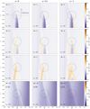 |
Fig. C.2 Same as Fig. C.1 but for St = 3, 4, 5, and 10. |
| In the text | |
|
Fig. D.1 Comparison of gas density distributions in NBR and BR models for St = 0.01, 0.1, 1, and 2, with three different accretion efficiencies (η = 0, 0.1, and 1), in the vicinity of 1 M⊕ planet. The axes are shown in code units. Colors ranging from blue to red represent increasing gas densities in the BR models. Regions where the two models agree are show in white. The black circle indicates the planetary Hill sphere. Note that the density ratios are multiplied by 1000 for clarity. |
| In the text | |
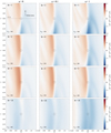 |
Fig. D.2 Same as Fig. D.1 but for St = 3, 4, 5, and 10. |
| In the text | |
Current usage metrics show cumulative count of Article Views (full-text article views including HTML views, PDF and ePub downloads, according to the available data) and Abstracts Views on Vision4Press platform.
Data correspond to usage on the plateform after 2015. The current usage metrics is available 48-96 hours after online publication and is updated daily on week days.
Initial download of the metrics may take a while.