| Issue |
A&A
Volume 694, February 2025
|
|
|---|---|---|
| Article Number | A286 | |
| Number of page(s) | 8 | |
| Section | Cosmology (including clusters of galaxies) | |
| DOI | https://doi.org/10.1051/0004-6361/202452707 | |
| Published online | 20 February 2025 | |
Blue monsters at z > 10: Where all their dust has gone
1
Scuola Normale Superiore, Piazza dei Cavalieri 7, 56126 Pisa, Italy
2
Center for Computational Astrophysics, Flatiron Institute, 162 5th Avenue, New York, NY 10010, USA
⋆ Corresponding author; This email address is being protected from spambots. You need JavaScript enabled to view it.
Received:
22
October
2024
Accepted:
7
January
2025
Abstract
The properties of luminous, blue, super-early galaxies (a.k.a. blue monsters) at redshift z > 10 have been successfully explained by the attenuation-free model (AFM), in which dust is pushed to kiloparsec scales by radiation-driven outflows. As an alternative to AFM, here we assess whether “attenuation-free” conditions can be replaced by a “dust-free” scenario in which dust is produced in very limited amounts and/or later destroyed in the interstellar medium. To this aim, we compare the predicted values of the dust-to-stellar mass ratio, ξd, with those measured in 15 galaxies at z > 10 from James Webb Space Telescope (JWST) spectra, when outflows are not included. Our model constrains ξd as a function of several parameters by allowing wide variations in the initial mass function (IMF), dust and metal production, and dust destruction for a set of supernova (SN) progenitor models and explosion energies. We find that log ξd ≈ −2.2 for all systems, which is indicative of the dominant role of SN dust production over destruction in these early galaxies. Such a value is strikingly different from the data, which instead indicates log ξd ≲ −4. We conclude that dust destruction alone can hardly explain the transparency of blue monsters. Other mechanisms, such as outflows, might be required.
Key words: galaxies: high-redshift / galaxies: ISM
© The Authors 2025
 Open Access article, published by EDP Sciences, under the terms of the Creative Commons Attribution License (https://creativecommons.org/licenses/by/4.0), which permits unrestricted use, distribution, and reproduction in any medium, provided the original work is properly cited.
This article is published in open access under the Subscribe to Open model. This email address is being protected from spambots. You need JavaScript enabled to view it. to support open access publication.
1. Introduction
In just two years of operations, the James Webb Space Telescope (JWST) has dramatically boosted the exploration of the early Universe. One of the major discoveries is a large number of super-early (z > 10) galaxies (Naidu et al. 2022; Arrabal Haro et al. 2023; Hsiao et al. 2023; Wang et al. 2023a; Fujimoto et al. 2023; Atek et al. 2022; Curtis-Lake et al. 2023; Robertson et al. 2023; Bunker et al. 2023; Tacchella et al. 2023; Arrabal Haro et al. 2023; Finkelstein et al. 2023; Castellano et al. 2024; Zavala et al. 2024; Helton et al. 2024; Carniani et al. 2024a; Robertson et al. 2024) that challenge expectations based on pre-JWST data, theoretical predictions, and perhaps even ΛCDM-based1 galaxy formation scenarios.
Super-early galaxies are characterized by bright UV luminosities (MUV ≲ −20), steep UV spectral slopes (β ≲ −2.2, Topping et al. 2022; Cullen et al. 2024; Morales et al. 2024), compact sizes (effective radius of re ≈ 200 pc, Baggen et al. 2023; Morishita et al. 2024; Carniani et al. 2024a), and large (for their epoch) stellar masses (M⋆ ≈ 109 M⊙, Castellano et al. 2024; Carniani et al. 2024a; see Table 1 for all the values). These properties have earned them the nickname of blue monsters (Ziparo et al. 2023). Their large comoving number density (n ≈ 10−5 − 10−6 cMpc−3, see e.g., Casey et al. 2024; Harvey et al. 2024) is very hard to explain in the framework of standard, pre-JWST models.
Relevant properties of spectroscopically confirmed super-early galaxies at z > 10.
These additions include (a) star formation variability (Furlanetto & Mirocha 2022; Mason et al. 2023; Mirocha & Furlanetto 2023; Sun et al. 2023; Pallottini & Ferrara 2023), (b) reduced feedback, resulting in a higher star formation efficiency (Dekel et al. 2023; Li et al. 2024), (c) a top-heavy initial mass function (IMF) (Inayoshi et al. 2022; Wang et al. 2023b; Trinca et al. 2024; Hutter et al. 2025) (although see Cueto et al. (2024)), and more exotic solutions, such as (d) the modification of ΛCDM via the presence of primordial black holes (Liu & Bromm 2023).
As a final possibility, we list the so-called “attenuation-free model” (AFM, Ferrara et al. 2023; Ziparo et al. 2023; Fiore et al. 2023; Ferrara 2024a,b), for which bright luminosities and blue colors result from extremely low dust attenuation conditions. According to AFM, dust is produced by stars in “standard” net2 amounts (i.e., dust-to-stellar ratios of ξd ∼ 0.001 − 0.01, see e.g. Inami et al. 2022; Sommovigo et al. 2022; Dayal et al. 2022; Witstok et al. 2023; Algera et al. 2024 for constraints up to z ∼ 7) and later pushed by outflows on kiloparsec scales. In this scenario, dust is not destroyed, but simply moved to distances such that the attenuation is decreased to the observed value (for a fixed dust mass, AV ∝ 1/r2, where r is the galactocentric radius). Interestingly, such a conclusion has been independently reached by Zhao & Furlanetto (2024).
The solution proposed by AFM is based on the notion that, due to their large specific star formation rates (SFRs), early galaxies can go through super-Eddington phases in which they launch powerful outflows driven by radiation pressure onto dust (Ziparo et al. 2023; Fiore et al. 2023; Ferrara 2024a). The AFM consistently explains the shape of the UV luminosity functions (Ferrara et al. 2023), the evolution of the cosmic SFR density (Ferrara 2024a), and the star formation history and properties of individual galaxies (Ferrara 2024b), induces a star formation mini-quenching (Gelli et al. 2023), and makes specific predictions for Atacama Large Millimeter Array (ALMA) targeted observations (Ferrara et al. 2025).
In spite of this success, it is important to consider alternatives to the AFM. Here, we instead postulate that the surviving dust amount is low enough to satisfy the experimental AV bound. Instead of invoking outflows, this can be achieved by (a) decreasing the net supernova (SN) yield, or (b) by increasing the destruction rate by interstellar shocks once grains are injected in the interstellar medium (ISM). The physics governing these processes is understood, but it depends on parameters that are only partially constrained (Dwek 1998; Bianchi & Schneider 2007; Martínez-González et al. 2019; Sarangi et al. 2018; Slavin et al. 2020; Kirchschlager et al. 2024; Narayanan et al. 2024).
In the present study, our aim is to assess whether attenuation-free conditions can be soundly replaced by dust-free conditions in which dust has either been produced in very limited amounts or destroyed thereafter. To answer this question, it is necessary to perform a thorough evaluation of the production and destruction processes that take place during the evolution of the galaxy, including extensive coverage of the free-parameter space.
We anticipate that our study concludes that dust-free conditions are hardly established without running into severe conflicts with observed physical conditions and observational bounds existing across comic epochs. This makes it difficult to consider (almost) dust-free conditions as a valid alternative to AFM in order to explain the properties of blue monsters.
2. Data
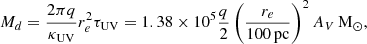
Super-early galaxies are characterized by very low dust-to-stellar mass ratios. To support this statement, we have collected a sample of currently available spectroscopic data, obtained by JWST/NIRspec observations, for 15 galaxies at z > 10 listed in Table 1. For each of them, the stellar mass, M⋆, has been derived by different authors by fitting the spectral energy distribution. The results are reported in column 8 of the Table; masses are in the range of 107.5−9.05 M⊙. The same fitting procedure also yields the V-band dust attenuation, AV (column 3). The effective stellar radius, re (column 5), was instead estimated from JWST/NIRcam photometric data.
To obtain the dust mass, we used the standard formula (see e.g. Ferrara 2024a)
 (1)
(1)
where q = (1, 2) for (disk, spherical) geometry, and κUV = 1.26 × 105 cm2 g−1 and τUV = 2.655 × (1.086AV) are the dust mass absorption coefficient for a Milky Way extinction curve (Weingartner & Draine 2001), and the optical depth at 1500 Å, respectively; the pre-factor 2.655 for τUV accounts for the differential attenuation between 1500 Å and the V band for the adopted extinction curve. We conservatively assume spherical geometry (q = 2) as in this case Md is maximized for a given measured AV.
The data implies that Md for all galaxies is generally very low (see Table 1), with the dustiest galaxy, CEERS2-7929, showing a scant dust mass of 5.2 × 10⁴ M⊙; other galaxies are virtually dust-free, featuring upper limits as low as 67 M⊙ (MACS0647-JD). Such dust scarcity determines the uncommonly low values of the dust-to-stellar ratios, ξd = Md/M⋆, which are shown as blue points in Fig. 2. The data indicates that log ξd is in the range from −6.27 to −3.51. For comparison, in Fig. 2 we also show the Milky Way value, log ξd = −3.2, and the ξd interval measured for 14 REBELS galaxies at z ≈ 7. Interestingly, galaxies in the REBELS sample (Bouwens et al. 2022) have a higher dust-to-stellar mass ratio, log ξd ≈ −2 (Ferrara et al. 2022; Dayal et al. 2022; Sommovigo et al. 2022). This conclusion has recently also been supported by those few galaxies having multiple-frequency dust continuum observations (Bakx et al. 2021; Witstok et al. 2023; Algera et al. 2024). Notably, numerical simulations (see e.g., Choban et al. 2024) fall more than 1 dex short in reproducing the observed dust masses.
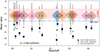 |
Fig. 2. Violin plots showing the posterior distribution of ξd resulting from the random sampling of the parameter space (see details in Sect. 5) for 15 super-early galaxies whose redshifts is indicated on the horizontal axis and whose name is shown at the top. For each galaxy, the red point represents the distribution median value; the horizontal bars inside the violin indicate the 32nd and 68th percentiles. The predicted ξd values are for η = 0, i.e., when no galactic outflows are allowed. The blue diamonds are the observed dust-to-stellar mass ratios; the green stars are the predicted dust-to-gas ratio, 𝒟. The horizontal hatched red band shows the measured ξd interval for 14 REBELS galaxies at z ≈ 7 (Table 1 in Ferrara et al. 2022; see also Dayal et al. 2022; Sommovigo et al. 2022; Inami et al. 2022). |
Thus, super-early galaxies (z > 10) have a dramatically lower dust content compared to expectations from known Epoch of Reionization (EoR) (z ≈ 7) and local galaxies. To gain some insight into such a fundamental issue, we developed the dust evolution model described below.
3. Model
To predict the dust mass of super-early galaxies and their dust-to-stellar mass ratio, we followed Ferrara (2024b) and wrote the evolutionary equations governing these two quantities, along with the analogous ones for the metal, MZ, and gas, Mg, mass:
![Mathematical equation: $$ \begin{aligned} \dot{M}_d(t)&= [y_d\nu - {{\mathcal{D} }}(t)(1+\beta +\eta ) ] \psi (t), \end{aligned} $$](/articles/aa/full_html/2025/02/aa52707-24/aa52707-24-eq74.gif) (2)
(2)
 (3)
(3)
-\eta \} \psi (t), \end{aligned} $$](/articles/aa/full_html/2025/02/aa52707-24/aa52707-24-eq76.gif) (4)
(4)
![Mathematical equation: $$ \begin{aligned} \dot{M}_g(t)&= f_b \dot{M}_a(t) -[(1-R)+\eta ] \psi (t) .\end{aligned} $$](/articles/aa/full_html/2025/02/aa52707-24/aa52707-24-eq77.gif) (5)
(5)
The function  denotes the SFR. Such a process occurs with an “instantaneous” efficiency, ϵ⋆, per free-fall time, tff = ζH(z)−1, where ζ = 0.06 and H(z)−1 is the Hubble time (Ferrara et al. 2023). Such efficiency implicitly encapsulates the effects of SN feedback in regulating and suppressing star formation.
In Eq. (2) yd is the “net;” that is, including the reverse shock destruction of the newly formed grains, the dust yield per SN formed per unit stellar mass, ν. Both yd and ν depend on IMF and other parameters; we defer their description to Sect. 5.
Dust sinks (second term in Eq. (2), r.h.s.) depend on the dust-to-gas ratio, 𝒟 = Md/Mg. Dust can be removed from the gas by astration, destroyed by SN interstellar shocks, and ejected by outflows. These terms are all proportional to ψ, with coefficients (1, β, η), respectively. The destruction coefficient, β, is rather uncertain, and its treatment is discussed in Sect. 5. As the aim of this work is to test alternative explanations to (radiation-driven) outflows for the observed UV transparency of blue monsters, we set the outflow loading factor to η = 0 in the following (see Pallottini et al. 2024 for the effect of outflows on the mass-metallicity relation).
Eq. (2) implicitly assumes that: (a) SNe are the only sources of dust at high z (Todini & Ferrara 2001; Leśniewska & Michalowski 2019; Ferrara et al. 2022); and (b) grain growth in the ISM can be neglected as its timescale is comparable to the Hubble time (Ferrara et al. 2016; Dayal et al. 2022). Including grain growth would increase Md, exacerbating the discrepancy with observations (see below); hence, our choice is conservative.
Eq. (3) expresses the fact that stellar mass increases with the SFR with a proportionality constant (1 − R) that is dependent on the gas return fraction3 of stars, R. In turn, R depends on IMF, as we detail in Sect. 4.
The last two equations (Eqs. (4)–(5)) describe the evolution of the metal and gas mass, respectively. The quantity yZ is the metal yield per SN; similarly to the dust yield, it depends on the IMF (Sect. 5). Depending on the metallicity, Z = MZ/Mg, a fraction of the heavy elements is swallowed by star formation. The gas mass increases at a rate of fbMa, where fb = Ωb/Ωm is the cosmological baryon fraction, and the dark matter halo growth is fed by cosmological accretion, whose rate (in M⊙ yr−1) is obtained from numerical simulations; for example Correa et al. (2015),
![Mathematical equation: $$ \begin{aligned} \dot{M}_a(M,z) = 102.2\, h [-a_0 -a_1 (1+z)] E(z) M_{12} .\end{aligned} $$](/articles/aa/full_html/2025/02/aa52707-24/aa52707-24-eq79.gif) (6)
(6)
The parameters (a0, a1) depend on the halo mass, M(z), cosmology, and the linear matter power spectrum, and are provided4 in Appendix C of Correa et al. (2015); E(z) = [Ωm(1 + z)3 + ΩΛ)]1/2, and M12 = M/1012 M⊙. Finally, gas is consumed by star formation and partly returned to the ISM (last term in Eq. (5)).
For later use, it is convenient to rewrite the accretion term, fb Ṁa, as a(z)ψ, with a(z) to be defined5. To this aim, we used the expression of ψ given in Eq. (5) to substitute for halo mass in Eq. (6), finally obtaining
![Mathematical equation: $$ \begin{aligned} a(z, \epsilon _\star ) = 6.23[-a_0 -a_1 (1+z)]\left(\frac{0.01}{\epsilon _\star }\right) .\end{aligned} $$](/articles/aa/full_html/2025/02/aa52707-24/aa52707-24-eq80.gif) (7)
(7)
For reference, a(z = 10)≃50(0.01/ϵ⋆); that is, the accretion rate largely exceeds the SFR (unless ϵ⋆ ≳ 0.5). In these conditions, the gas fraction is fg = Mg/(Mg + M⋆)≃1, and Mg ≈ fbM.
4. Analytical insights
While is it possible to solve the evolutionary Eqs. (2)–(5) numerically, as was done in Ferrara (2024b), to gain a deeper physical insight into dust enrichment we seek here analytical solutions. To fix ideas, in this section for numerical estimates we have adopted fiducial values for the five parameters of the model. These are: ν−1 = 52.89 M⊙, R = 0.61, yd = 0.1 M⊙, yZ = 2.41 M⊙, and β = 4.7. A detailed discussion of these parameters and their uncertainties is given in Sect. 5; the effects on the final results of their combined variation are presented in Sect. 6.
4.1. Whether SNe are predominantly dust sources or sinks
First, we note from Eq. (2) that SNe act both as dust sources and sinks. Dust is produced immediately (a few hundred days) after the explosion in the expanding SN envelope, where it is also processed by the reverse shock thermalizing the ejecta. Behind the forward shock propagating in the ISM, preexisting dust is partially destroyed by sputtering and shattering.
To assess whether SNe are net dust producers or destroyers, we took a closer look at Eq. (2). By comparing the two competing terms, we concluded that SNe are net dust producers as long as
 (8)
(8)
For the numerical estimate, we used the fiducial values of the parameters; the adopted value of the Milky Way dust-to-gas ratio is 𝒟MW = 1/162 (Rémy-Ruyer et al. 2014). Thus, in the early evolutionary stages, when 𝒟 is low, SNe are net dust sources. In more evolved galaxies, they predominantly destroy the dust created by other sources (AGB and late-type stars) or processes (such as grain growth).
We pause to emphasize an important fact. A key difference between dust destruction (β) and outflows (η) is that while sputtering and shocks destroy dust, outflows simply carry it away from stars. Hence, the value of ξd depends on the physical scale on which it is measured. In other words, although the β and η enter Eq. (2) as an additive term, destruction and outflows do not have the same physical consequences.
We can also translate the above condition into one on metallicity, by adopting a 𝒟 − Z relation, which we took6 from (Rémy-Ruyer et al. 2014, see also Lisenfeld & Ferrara 1998). These authors found that 𝒟 = (Z/Z⊙)1.62 𝒟MW, where Z⊙ = 0.0142 (Asplund et al. 2009). Hence, 𝒟crit = 0.05𝒟MW would correspond to Zcrit = 0.16 Z⊙. From Table 1, we see that none of the super-early galaxies has Z > Zcrit. We conclude that their dust is consistently produced by SNe, and inefficiently destroyed in the ISM.
4.2. A closed-form solution
To obtain a closed-form solution for ξd, we considered Eqs. (2) and (3). With simple algebraic manipulations, and using the definition of 𝒟crit in Eq. (8), we find that the dust-to-stellar mass ratio can be written as
![Mathematical equation: $$ \begin{aligned} \xi _d&= \frac{1}{y} \left[ 1 - \exp {(-\xi _d^0 y})\right],\end{aligned} $$](/articles/aa/full_html/2025/02/aa52707-24/aa52707-24-eq82.gif) (9)
(9)
 (10)
(10)
We have introduced the production-only dust-to-stellar mass ratio ξd0 = ydν/(1 − R). The value ξd would be attained if dust were not post-processed in the ISM by astration or destruction (or growth).
We first notice that in the limiting case M⋆/Mg ≪ 1 (gas-dominated systems), using the fiducial values of the parameters, log ξd ≃ log ξd0 = −2.2, a value ≥100 higher than inferred for super-early galaxies (Fig. 2).
A general use of Eq. (9) requires instead an estimate of M⋆/Mg. As M⋆ is known for these galaxies, to make progress we need to constrain Mg. At the moment, detailed information on the gas content of z > 10 galaxies is lacking. This will have to await for ALMA observations of these systems; in particular, the [CII]158μm line appears to be the best gas tracer (Zanella et al. 2018).
Fortunately, though, we can use the metallicity data7 provided by the exquisite JWST spectra to obtain Mg. To this aim, we considered the other two equations (Eqs. (4) and (5)) in the system. With simple algebra, it is easy to show that the gas metallicity of a purely accreting, star-forming galaxy with no outflows (η = 0) is
![Mathematical equation: $$ \begin{aligned} Z = y_Z\nu \frac{(1-R)}{a(z,\epsilon _\star )} \left[1-\left(\frac{M_g}{M_0} \right)^{a/q}\right] \simeq y_Z\nu \frac{(1-R)}{a(z,\epsilon _\star )}. \end{aligned} $$](/articles/aa/full_html/2025/02/aa52707-24/aa52707-24-eq84.gif) (11)
(11)
Here, we have introduced q = 1 − R − a ≈ −a as a ≫ (1 − R) (see Eq. (7)); hence, a/q ≈ −1. The last equality comes instead from the fact that the gas mass at the final redshift is much larger than what is available when star formation begins, M0. Canonically, this epoch coincides with the moment at which the halo growth crosses the value M ≃ 108 M⊙, marking the boundary of the atomic cooling regime (virial temperature T > 104 K).
By noting8 that M⋆ = (1 − R)ϵ⋆Mg, and using the result obtained in Eq. (11) we can write that
 (13)
(13)
having also used a(z = 10, ϵ⋆)≃1/2ϵ⋆ (see Eq. (7)).
To obtain the small observed values, ξd ≃ 10−5, the quantity  in Eq. (9) has to be large. In this case, the equation simplifies and becomes (using fiducial values of the parameters)
 (14)
(14)
Hence, imposing ξd ≃ 10−5, and given the average metallicity of the sample Z ≃ 0.05 Z⊙, it should be 𝒟crit ≃ 8 × 10⁻⁸. This low 𝒟crit value would require an unphysically high value β ≃ 2.3 × 10⁴. Such a destruction efficiency is orders of magnitude higher than what is predicted by all dust destruction models and observations, as is discussed in Sect. 5.
4.3. Star formation efficiency
We conclude this section by emphasizing that high star formation efficiencies necessarily imply large metallicities (see Eq. (11)). For the fiducial value yZ = 2.41 M⊙, we find that at z = 10, Z = 0.02(ϵ⋆/0.01)Z⊙. Hence, the metallicity of all galaxies in Table 1 can be matched with small variations in the efficiency in the range of 0.01 − 0.05. Larger star formation efficiencies would dramatically overproduce the predicted metallicities with respect to the observed ones. We recall that, by choice, the scenario investigated here does not include outflows.
We also note that, as a(z, ϵ⋆) depends linearly on redshift, the metallicity grows with time. For example, the same calculation performed at z = 2 yields Z = 0.08(ϵ⋆/0.01)Z⊙.
5. Model parameters
Eq. (9) contains a number of parameters that we have allowed to vary. These are: ν, R, yd, yZ, and β. So far, for our estimates we have used fiducial values for these parameters, but it is important to assess the impact of their combined variation. As was already mentioned, the first four depend on the IMF and on the SN progenitor properties (rotation, explosion energy); the dust yield, yd, also depends on the ISM gas density affecting the reverse shock destruction efficiency. Finally, β controls dust destruction by shocks in the ISM. We discuss how we model these processes in the following.
5.1. Initial mass function
We assumed that stars form with masses in the range (ml, mu) = (0.1, 100)M⊙ according to a Larson IMF (Larson 1998) normalized to unity in the above range9, which follows a Salpeter-like power law at the upper end but flattens below a characteristic stellar mass:
 (15)
(15)
where α = 1.35. We take mc to be a random variable log-normally distributed with mean and standard deviation (μ1, σ1) = (0, 0.5) (an example of a random distribution is shown in Fig. 1). Assuming that stars with m > 8 M⊙ explode as SNe, we derive the number of SNe per unit stellar mass formed, ν, as a function of mc.
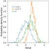 |
Fig. 1. Example of a probability density function for three parameters of the problem, the IMF characteristic mass, mc, the ISM gas density, ng, and the destruction coefficient, β. These are discussed in Sect. 5.1, Sect. 5.2, and Sect. 5.4, respectively. |
Imposing the instantaneous recycling approximation (Maeder 1992), for which stars with a mass of m < m0 (m ≥ m0) live forever (die immediately), the return fraction, R, is
 (15)
(15)
We fixed m0 = 2.3 M⊙, the mass of a star whose lifetime is equal to the cosmic age (483 Myr) at z = 10, and assumed (Weidemann 2000) that the remnant mass is (a) wm = 0.444 + 0.084m for m < 8 M⊙; (b) wm = 1.4 M⊙ (neutron star) for 8 M⊙ < m < mBH = 40 M⊙, and (c) wm = m for m > mBH when they collapse into a black hole.
5.2. Dust yields
To compute the dust, yd, yields from SNe, it is necessary to define the stellar progenitor model. In general, the nucleosynthetic yields depend on the explosion energy and on the possible rotation of the star. We followed Marassi et al. (2019, see their Tables 9–12) who considered four different models. The first two models assumed a fixed explosion energy of 1051 erg, and the star was either nonrotating (FE-NR) or rotating (FE-ROT) at a velocity of 300 km s−1. Instead, the second set adopted a variable explosion energy calibrated to reproduce the amount of 56Ni obtained from the best fit to the observations for nonrotating (CE-NR) or rotating (CE-ROT) progenitors10. In all cases, the metallicity was fixed to 0.01 Z⊙. Marassi et al. (2019) performed detailed dust nucleation calculations and obtained yd for the four models above for 10 different progenitor masses in the range 8 − 120 M⊙. The computed dust yields are in the range of ≈0.1 − 1.4 M⊙, with the CE-ROT predicting the highest values (with the notable exception of the 60 M⊙ star producing up to 7.4 M⊙ of dust in this case). In our sampling of the parameter space, the stellar model was set by assuming that (FE-NR, FE-ROT, CE-NR, CE-ROT) are distributed as a uniform discrete random variable.
Marassi et al. (2019) did not consider the processing of the newly formed grain by the reverse shock thermalizing the ejecta. We therefore augmented their model with the results by Nozawa et al. (2007), who computed the surviving dust mass fraction after the reverse shock, frev, for a range of masses from 13 to 200 M⊙ and for a range of environmental gas densities in which the explosion takes place, from ng = 0.1 to 10 cm−3. We linearly interpolated their results on our progenitor masses and gas densities. We further assumed the unmixed ejecta case. We point out that Nozawa et al. (2007) results are strictly valid in the FE-NR case only; lacking more general computations, we adopted them for all four stellar progenitor models.
We took ng to be a random variable that is log-normally distributed with mean and standard deviation (μ3, σ3) = (0.5, 0.5) (see Fig. 1). It is important to note that the mean gas density of early galaxies is thought to be larger than locally (Isobe et al. 2023), reaching values of ≈103 cm−3 at z ≳ 10. Nevertheless, the explosion is always going to occur in a relatively low (1 − 10 cm−3) density medium.
To see this, we assumed that at the star birth the gas density is ng0 = 103 cm−3. Due to the strong ionizing power of the massive (m > 8 M⊙) SN progenitor, an H II region will form. The Strömgren radius will be filled in a recombination time, or (ng0αB)−1 ≃ 120 yr, where αB is the case-B recombination coefficient of H-atoms. From that moment, the over-pressurized H II region (temperature Ti ≈ 2 × 10⁴ K) will start to expand to restore pressure equilibrium with the surrounding gas. The external gas temperature in an almost metal-free gas was set by molecular hydrogen to T0 ≲ 300 K; if the metallicity were higher, the gas could be even colder. Then the expansion would decrease the density by a factor of Ti/T0, bringing it down to ng ≲ 15 cm−3.
This simple estimate is in line with radiative transfer simulations (e.g., Whalen et al. 2004) of HII regions around massive stars. These authors find that even starting from initial gas densities well in excess of 103 cm−3, the HII regions produce an almost uniform distribution of the gas around the stars. They find (see their Fig. 3) that the density in the HII region is ≈0.1 cm−3 after 2.2 Myr; that is, approximately the time when the most massive stars explode as SNe. This justifies our choice for the mean value, μ3, of the gas density, which we allowed nevertheless to vary considerably to catch the uncertainties in the gas and stellar properties.
As a reference, according to Nozawa et al. (2007) results, the surviving dust mass fraction for ng ≈ 1 (10) cm−3 varies from 20 to 47 (4 to 10) percent in the mass range of 8 M⊙ < m < 40 M⊙. We performed a 2D linear interpolation in the stellar mass – gas density plane to derive frev when sampling our model.
5.3. Metal yields
To compute the metal yields, we followed Kim et al. (2014), who used the results by Woosley & Heger (2007). In practice, the oxygen and iron mass can be converted into a total metal mass using the following formula:
 (17)
(17)
where
 (18)
(18)
 (19)
(19)
Eq. (17) was then integrated over the IMF to obtain the metal yield yZ, the average metal mass produced per SN. In the fiducial case, yZ = 2.41 M⊙; this result is very weakly dependent on the metallicity of the stars. We warn, however, that Woosley & Heger (2007) results have been computed for the standard case FE-NR, and we are applying them also to the other three progenitor models adopted here.
5.4. Dust destruction in interstellar shocks
In addition to reverse shocks discussed in Sect. 5.2, grains can be destroyed in interstellar shocks produced by SNe (see Sect. 4.1) for a discussion of the required conditions). As a result, the destruction term is proportional to the SFR, ψ, via a destruction coefficient, β (Eq. (2)). The coefficient is itself the product of different terms (e.g. Dayal et al. 2022):
 (20)
(20)
In the previous equation, νMsdest is the mass of gas in which dust is destroyed by the SN shocks per unit stellar mass formed. A value of  has been estimated by Slavin et al. (2015) by assuming a 50%+50% mixture of silicate and carbonaceous grains. Bocchio et al. (2014) found instead a ≈2.6 times larger value (for silicates) due to the fact that they assume a different grain destruction efficiency as a function of the shock velocity.
The other two factors in Eq. (20) represent the fraction of SNe exploding outside the galaxy main body, δSN ≃ 0.36, and the fraction of warm (≈8000 K) to hot gas in the galaxy, feff ≃ 0.43 (Slavin et al. 2015). These quantities have been calibrated locally (Schneider & Maiolino 2024), and are therefore somewhat uncertain. At face value, they would give a fiducial value of β = 4.7. In view of these uncertainties, we take β to be a random variable that is log-normally distributed with a mean and standard deviation (μ4, σ4) = (0.7, 0.3) (see Fig. 1).
To summarize, our model contains five parameters that we have allowed to vary to fully sample the physical uncertainties related to their value in early galaxies. These are: ν, R, yd, yZ, β. For each galaxy, we ran N = 1000 models11, each for a random combination of the parameters, and thus fully sampled the parameter space determining the value of the dust-to-stellar mass ratio obtain in Eq. (9). As is seen from Fig. 1, each parameter can take values in a wide range spanning 2 − 3 orders magnitude around the mean. We recall that in addition to these parameters, we considered four different randomly selected stellar models for the SN progenitor (see Sect. 5.2).
6. Results
The results of our study are condensed in Fig. 2. There, we show the violin plot for the posterior distribution of ξd resulting from the random sampling of the parameter space for each of the 15 super-early galaxies. The red point in each distribution represents the median value; also shown with horizontal bars inside the violins are the 32th and 68th percentiles.
The median values of all the galaxies are rather similar and fall in a narrow range around log ξd = −2.2. This fact is indicative that the value of the dust-to-stellar ratio is largely determined by the net (i.e., including the reverse shock destruction) SN dust yield, with the destruction in interstellar shocks being negligible. This result confirms the conclusion drawn in Sect. 4.1, where we show that for 𝒟 < 𝒟crit ≈ 3 × 10⁻⁴ SNe largely act as dust sources rather than sinks. Indeed, the values that we predict for the dust-to-gas ratio, 𝒟, in z > 10 systems (green stars in Fig. 2) are consistently below 10−4. The distributions are somewhat skewed toward low ξd, with some model combinations yielding ξd ≈ 10−4 for most extreme values of the parameters.
The difference between the predicted ξd values and the measured ones (blue diamonds) is striking. Apparently, no combination of parameters, although they have been allowed to vary in a large range around the fiducial values given in the literature, yields ξd < 10−4, while the majority of the data points are well below that threshold. Three galaxies (CEERS2-7929, UNCOVER-37126, and UNCOVER-z12) have a measured ξd > 10−4, but are still several r.m.s. away from the predicted median. The discrepancy is even more impressive for the most well-studied galaxies, such as GHZ2, GS-z11-0, and GS-z13-0, for which exquisite-quality spectra are available. These systems show dust-to-stellar ratios as low as ξd ≈ 10−6.
Thus, it appears that the blue colors (steep UV slopes) and transparency (low AV) of super-early galaxies imply extremely low dust-to-stellar mass ratios that cannot be reproduced by “standard” dust physics (in the absence of outflows), even allowing for a large and simultaneous variation range for all the (admittedly uncertain) dust production and destruction parameters. One could be tempted to dramatically change the dust yields or make the dust destruction extremely efficient. However, going down that path, we would be faced with the difficulty of explaining a large body of data for local galaxies, and their intermediate- and high-z counterparts (such as the REBELS galaxy sample at z ≈ 7), which are well explained by the present model.
7. Summary and discussion
As a test of the AFM, we have compared the predicted values of the dust-to-stellar mass ratio, ξd, measured in 15 z > 10 galaxies with those derived from JWST spectra. Unlike AFM, the model considered here does not rely on outflows to remove dust from the galaxy main body. Instead, it constrains the value of ξd as a function of various parameters (this is discussed in detail in Sect. 5) by allowing variations in the IMF, dust and metal production, and dust destruction for a set of SN progenitor stellar models.
The key results are shown in Fig. 2. We see that the predicted ξd range is around log ξd = −2.2 for all galaxies, which is indicative of the dominant role of SN dust production over destruction in these early systems. The predictions are strikingly different from the data, which instead show values of log ξd ≲ −4. We conclude that negligible dust production or strongly enhanced destruction can hardly reconcile theory and observations without conflicting with well-studied z ≈ 7 − 8 galaxies. Other mechanisms, such as outflows, might be required by this evidence.
In this study, we have purposely not allowed for the occurrence of outflows, although cosmological infall has been included in our master Eqs. (2)–(5). Our aim has been to challenge the AFM by proposing a radically different solution to the overabundance and colors of bright super-early galaxies.
The AFM scenario (Ferrara 2024a,b) suggests that if dust could be lifted out of the main galaxy body and into its halo on kiloparsec scales, the low AV values could be readily explained by the 1/r2 decrease in the dust column density. This hypothesis is supported by the fact that, toward high z, outflows become more common as a result of the increased compactness of galaxies and their on-average larger specific SFR (sSFR). Both these conditions favor powerful radiation-driven outflows clearing the dust (Ziparo et al. 2023; Fiore et al. 2023; Ferrara 2024a).
In AFM, dust “standard” formation and evolution physics still holds, but dust is dispersed by outflows mimicking a lack of dust, and producing the low observed attenuation (see the case of GS-z14-0 in Ferrara 2024b). Thus, a no-outflow model, such as the one presented here, falls far short of reproducing the data, which instead are well reproduced by the AFM. It is worth noting that, in an independent study based on CROC simulations, Esmerian & Gnedin (2024) find that models successfully fitting the total dust mass and infrared luminosities of super-early galaxies produce far too much attenuation in the UV. This conclusion is in perfect agreement with what is found here.
Interestingly, the larger and more evolved REBELS galaxies (z ≈ 7) show ξd values of the same order (≈1/100) as is predicted here (Ferrara et al. 2022; Dayal et al. 2022; Algera et al. 2024). This might indicate that the processes included in this study – in the absence of powerful outflows – continue to regulate the dust abundance for a long cosmic time stretch. Intriguingly, their measured metallicities and gas fractions can be generally explained by a no-outflow model (Algera et al., in prep.), which entails the high ξd predicted here.
It is worth noticing that we have neglected dust growth. Although likely not important at these early redshifts due to the long associated timescales (Dayal et al. 2022) or prevailing physical conditions (Ferrara et al. 2016), dust growth would exacerbate the problem by increasing ξd even above the values found here.
On more general grounds, we note that blue monsters are characterized by a sustained SFR around 10−20 M⊙ yr−1. It is well established(e.g. McKee & Ostriker 2007; Glover & Clark 2012; Pallottini et al. 2022) that star formation can only occur if the star-forming gas is shielded from UV radiation by dust. It is therefore hard to understand how such an active star formation phase could have started and been supported in a virtually dust-free environment.
This work suggests that the dust we observe in blue monsters retains the properties of dust that has been freshly produced by a SN without significant reprocessing in the ISM. If correct, dust formation models (Todini & Ferrara 2001; Nozawa et al. 2007; Hirashita et al. 2015) predict that these readily produced grains should be large, with sizes in the range of 0.1 − 0.5 μm. This has also been confirmed experimentally by far-IR observations of nearby supernova remnants (Wesson et al. 2015; Priestley et al. 2020), and is in agreement with emission line extinction measurements (Gall et al. 2014; Bevan & Barlow 2016). In this case, we do expect the extinction curve to become almost frequency-independent (i.e., “gray”). This has indeed been recently found by Markov et al. (2024) using a sample of ≈100 JWST galaxy spectra in the redshift range of z = 2 − 11. Similar conclusions are reached by Langeroodi et al. (2024). Interestingly, the subsequent shattering of large grains into smaller ones could produce a reddening of the UV spectrum over time, and thus smoothly match the observed evolution (Narayanan et al. 2024).
Throughout the paper, we assume a flat Universe with the following cosmological parameters: ΩM = 0.3075, ΩΛ = 1 − ΩM, and Ωb = 0.0486, h = 0.6774, σ8 = 0.826, where ΩM, ΩΛ, and Ωb are the total matter, vacuum, and baryon densities, in units of the critical density; h is the Hubble constant in units of 100 km s−1, and σ8 is the late-time fluctuation amplitude parameter (Planck Collaboration XVI 2014).
That is, after reprocessing by the reverse shock thermalizing the ejecta.
We implicitly adopt the Instantaneous Recycling Approximation.
For reference, when averaged over 8 < log(M0/M⊙) < 14, (a0, a1) = (0.25, −0.75).
We computed a(z) at the observed galaxy redshift as the star formation histories of z > 10 galaxies are short (20 − 30 Myr). Hence, we neglected the small change in Ṁa in that time frame.
Rémy-Ruyer et al. (2014) give also an alternative broken power-law fit (see their Table 2) from which we find a similar result, Zcrit = 0.12 Z⊙.
For the three galaxies for which Z measurements are not available (see Table 1) we use the mean value of the sample.
In general, by time integration of Eq. (3), one would obtain
 (12)
(12)
where ⟨ϵ⋆⟩ is the gas conversion efficiency. If star formation lasts for about a free-fall time (≈30 Myr at z = 10), than ⟨ϵ⋆⟩≈ϵ⋆. Therefore, we neglect the small difference, and simply write M⋆ = (1 − R)ϵ⋆Mg.
Such a choice neglects the possible presence of pair instability SNe, which occur only in the range 140 − 260 M⊙ and possibly only at very low metallicity; therefore they are very rare. Moreover, they would further enhance dust and metals yields compared to core-collapse SNe, worsening the problem at hand.
We note that the black hole mass formation is mBH = 40 M⊙ for the standard FE-NR model, but it is larger for the other three models (mBH = 60 M⊙). This is taken into account in the calculation.
We have checked that the posterior distribution of ξd does not change significantly if N is increased.
Acknowledgments
We thank S. Carniani, M. Castellano, Y. Harikane, A. Inoue, F. Priestley for useful discussions, data and comments. This work is supported by the ERC Advanced Grant INTERSTELLAR H2020/740120. This research was supported in part by grant NSF PHY-2309135 to the Kavli Institute for Theoretical Physics (KITP). Plots in this paper produced with the MATPLOTLIB (Hunter 2007) package for PYTHON.
References
- Algera, H. S. B., Inami, H., Sommovigo, L., et al. 2024, MNRAS, 527, 6867 [Google Scholar]
- Arrabal Haro, P., Dickinson, M., Finkelstein, S. L., et al. 2023, arXiv e-prints [arXiv:2304.05378] [Google Scholar]
- Asplund, M., Grevesse, N., Sauval, A. J., & Scott, P. 2009, ARA&A, 47, 481 [NASA ADS] [CrossRef] [Google Scholar]
- Atek, H., Shuntov, M., Furtak, L. J., et al. 2022, arXiv e-prints [arXiv:2207.12338] [Google Scholar]
- Baggen, J. F. W., van Dokkum, P., Labbé, I., et al. 2023, ApJ, 955, L12 [NASA ADS] [CrossRef] [Google Scholar]
- Bakx, T. J. L. C., Sommovigo, L., Carniani, S., et al. 2021, MNRAS, 508, L58 [NASA ADS] [CrossRef] [Google Scholar]
- Bevan, A., & Barlow, M. J. 2016, MNRAS, 456, 1269 [NASA ADS] [CrossRef] [Google Scholar]
- Bianchi, S., & Schneider, R. 2007, MNRAS, 378, 973 [NASA ADS] [CrossRef] [Google Scholar]
- Bocchio, M., Jones, A. P., & Slavin, J. D. 2014, A&A, 570, A32 [NASA ADS] [CrossRef] [EDP Sciences] [Google Scholar]
- Bouwens, R. J., Smit, R., Schouws, S., et al. 2022, ApJ, 931, 160 [NASA ADS] [CrossRef] [Google Scholar]
- Bunker, A. J., Saxena, A., Cameron, A. J., et al. 2023, A&A, 677, A88 [NASA ADS] [CrossRef] [EDP Sciences] [Google Scholar]
- Carniani, S., Hainline, K., D’Eugenio, F., et al. 2024a, Nature, 633, 318 [CrossRef] [Google Scholar]
- Carniani, S., D’Eugenio, F., Ji, X., et al. 2024b, arXiv e-prints [arXiv:2409.20533] [Google Scholar]
- Casey, C. M., Akins, H. B., Shuntov, M., et al. 2024, ApJ, 965, 98 [NASA ADS] [CrossRef] [Google Scholar]
- Castellano, M., Napolitano, L., Fontana, A., et al. 2024, arXiv e-prints [arXiv:2403.10238] [Google Scholar]
- Choban, C. R., Salim, S., Kereš, D., Hayward, C. C., & Sandstrom, K. M. 2024, arXiv e-prints [arXiv:2408.08962] [Google Scholar]
- Correa, C. A., Wyithe, J. S. B., Schaye, J., & Duffy, A. R. 2015, MNRAS, 450, 1521 [NASA ADS] [CrossRef] [Google Scholar]
- Cueto, E. R., Hutter, A., Dayal, P., et al. 2024, A&A, 686, A138 [NASA ADS] [CrossRef] [EDP Sciences] [Google Scholar]
- Cullen, F., McLeod, D. J., McLure, R. J., et al. 2024, MNRAS, 531, 997 [NASA ADS] [CrossRef] [Google Scholar]
- Curtis-Lake, E., Carniani, S., Cameron, A., et al. 2023, Nat. Astron., 7, 622 [NASA ADS] [CrossRef] [Google Scholar]
- Dayal, P., Ferrara, A., Sommovigo, L., et al. 2022, MNRAS, 512, 989 [NASA ADS] [CrossRef] [Google Scholar]
- Dekel, A., Sarkar, K. C., Birnboim, Y., Mandelker, N., & Li, Z. 2023, MNRAS, 523, 3201 [NASA ADS] [CrossRef] [Google Scholar]
- Dwek, E. 1998, ApJ, 501, 643 [NASA ADS] [CrossRef] [Google Scholar]
- Esmerian, C. J., & Gnedin, N. Y. 2024, ApJ, 968, 113 [NASA ADS] [CrossRef] [Google Scholar]
- Ferrara, A. 2024a, A&A, 684, A207 [NASA ADS] [CrossRef] [EDP Sciences] [Google Scholar]
- Ferrara, A. 2024b, arXiv e-prints [arXiv:2405.20370] [Google Scholar]
- Ferrara, A., Viti, S., & Ceccarelli, C. 2016, MNRAS, 463, L112 [NASA ADS] [CrossRef] [Google Scholar]
- Ferrara, A., Sommovigo, L., Dayal, P., et al. 2022, MNRAS, 512, 58 [NASA ADS] [CrossRef] [Google Scholar]
- Ferrara, A., Pallottini, A., & Dayal, P. 2023, MNRAS, 522, 3986 [NASA ADS] [CrossRef] [Google Scholar]
- Ferrara, A., Carniani, S., di Mascia, F., et al. 2025, A&A, 694, A215 [NASA ADS] [CrossRef] [EDP Sciences] [Google Scholar]
- Finkelstein, S. L., Leung, G. C. K., Bagley, M. B., et al. 2023, arXiv e-prints [arXiv:2311.04279] [Google Scholar]
- Fiore, F., Ferrara, A., Bischetti, M., Feruglio, C., & Travascio, A. 2023, ApJ, 943, L27 [NASA ADS] [CrossRef] [Google Scholar]
- Fujimoto, S., Wang, B., Weaver, J., et al. 2023, arXiv e-prints [arXiv:2308.11609] [Google Scholar]
- Furlanetto, S. R., & Mirocha, J. 2022, MNRAS, 511, 3895 [NASA ADS] [CrossRef] [Google Scholar]
- Gall, C., Hjorth, J., Watson, D., et al. 2014, Nature, 511, 326 [CrossRef] [Google Scholar]
- Gelli, V., Salvadori, S., Ferrara, A., Pallottini, A., & Carniani, S. 2023, ApJ, 954, L11 [NASA ADS] [CrossRef] [Google Scholar]
- Glover, S. C. O., & Clark, P. C. 2012, MNRAS, 421, 9 [NASA ADS] [Google Scholar]
- Harikane, Y., Nakajima, K., Ouchi, M., et al. 2024, ApJ, 960, 56 [NASA ADS] [CrossRef] [Google Scholar]
- Harvey, T., Conselice, C., Adams, N. J., et al. 2024, arXiv e-prints [arXiv:2403.03908] [Google Scholar]
- Helton, J. M., Rieke, G. H., Alberts, S., et al. 2024, arXiv e-prints [arXiv:2405.18462] [Google Scholar]
- Hirashita, H., Ferrara, A., Dayal, P., & Ouchi, M. 2015, in Revolution in Astronomy with ALMA: The Third Year, eds. D. Iono, K. Tatematsu, A. Wootten, & L. Testi, ASP Conf. Ser., 499, 67 [NASA ADS] [Google Scholar]
- Hsiao, T. Y. Y., Abdurro’uf, Coe, D., et al. 2023, arXiv e-prints [arXiv:2305.03042] [Google Scholar]
- Hunter, J. D. 2007, Comput. Sci. Eng., 9, 90 [NASA ADS] [CrossRef] [Google Scholar]
- Hutter, A., Cueto, E. R., Dayal, P., et al. 2025, A&A, in press, https://doi.org/10.1051/0004-6361/202452460 [Google Scholar]
- Inami, H., Algera, H. S. B., Schouws, S., et al. 2022, MNRAS, 515, 3126 [NASA ADS] [CrossRef] [Google Scholar]
- Inayoshi, K., Harikane, Y., Inoue, A. K., Li, W., & Ho, L. C. 2022, ApJ, 938, L10 [NASA ADS] [CrossRef] [Google Scholar]
- Isobe, Y., Ouchi, M., Nakajima, K., et al. 2023, ApJ, 956, 139 [NASA ADS] [CrossRef] [Google Scholar]
- Kim, J.-H., Abel, T., Agertz, O., et al. 2014, ApJS, 210, 14 [Google Scholar]
- Kirchschlager, F., Sartorio, N. S., De Looze, I., et al. 2024, MNRAS, 528, 5364 [NASA ADS] [CrossRef] [Google Scholar]
- Langeroodi, D., Hjorth, J., Ferrara, A., & Gall, C. 2024, arXiv e-prints [arXiv:2410.14671] [Google Scholar]
- Larson, R. B. 1998, MNRAS, 301, 569 [NASA ADS] [CrossRef] [Google Scholar]
- Leśniewska, A., & Michałowski, M. J. 2019, A&A, 624, L13 [Google Scholar]
- Li, Z., Dekel, A., Sarkar, K. C., et al. 2024, A&A, 690, A108 [NASA ADS] [CrossRef] [EDP Sciences] [Google Scholar]
- Lisenfeld, U., & Ferrara, A. 1998, ApJ, 496, 145 [NASA ADS] [CrossRef] [Google Scholar]
- Liu, B., & Bromm, V. 2023, arXiv e-prints [arXiv:2312.04085] [Google Scholar]
- Maeder, A. 1992, A&A, 264, 105 [NASA ADS] [Google Scholar]
- Marassi, S., Schneider, R., Limongi, M., et al. 2019, MNRAS, 484, 2587 [NASA ADS] [CrossRef] [Google Scholar]
- Markov, V., Gallerani, S., Ferrara, A., et al. 2024, arXiv e-prints [arXiv:2402.05996] [Google Scholar]
- Martínez-González, S., Wünsch, R., Sommovigo, L., Silich, S., et al. 2019, ApJ, 887, 198 [CrossRef] [Google Scholar]
- Mason, C. A., Trenti, M., & Treu, T. 2023, MNRAS, 521, 497 [NASA ADS] [CrossRef] [Google Scholar]
- McKee, C. F., & Ostriker, E. C. 2007, ARA&A, 45, 565 [Google Scholar]
- McLure, R. J., Dunlop, J. S., Cullen, F., et al. 2018, MNRAS, 476, 3991 [Google Scholar]
- Mirocha, J., & Furlanetto, S. R. 2023, MNRAS, 519, 843 [Google Scholar]
- Morales, A. M., Finkelstein, S. L., Leung, G. C. K., et al. 2024, ApJ, 964, L24 [NASA ADS] [CrossRef] [Google Scholar]
- Morishita, T., Stiavelli, M., Chary, R.-R., et al. 2024, ApJ, 963, 9 [NASA ADS] [CrossRef] [Google Scholar]
- Naidu, R. P., Oesch, P. A., van Dokkum, P., et al. 2022, arXiv e-prints [arXiv:2207.09434] [Google Scholar]
- Narayanan, D., Stark, D. P., Finkelstein, S. L., et al. 2024, arXiv e-prints [arXiv:2408.13312] [Google Scholar]
- Nozawa, T., Kozasa, T., Habe, A., et al. 2007, ApJ, 666, 955 [NASA ADS] [CrossRef] [Google Scholar]
- Pallottini, A., & Ferrara, A. 2023, A&A, 677, L4 [NASA ADS] [CrossRef] [EDP Sciences] [Google Scholar]
- Pallottini, A., Ferrara, A., Gallerani, S., et al. 2022, MNRAS, 513, 5621 [NASA ADS] [Google Scholar]
- Pallottini, A., Ferrara, A., Gallerani, S., et al. 2024, A&A, submitted [arXiv:2408.00061] [Google Scholar]
- Planck Collaboration XVI. 2014, A&A, 571, A16 [NASA ADS] [CrossRef] [EDP Sciences] [Google Scholar]
- Priestley, F. D., Barlow, M. J., De Looze, I., & Chawner, H. 2020, MNRAS, 491, 6020 [NASA ADS] [CrossRef] [Google Scholar]
- Rémy-Ruyer, A., Madden, S. C., Galliano, F., et al. 2014, A&A, 563, A31 [Google Scholar]
- Robertson, B. E., Tacchella, S., Johnson, B. D., et al. 2023, Nat. Astron., 7, 611 [NASA ADS] [CrossRef] [Google Scholar]
- Robertson, B., Johnson, B. D., Tacchella, S., et al. 2024, ApJ, 970, 31 [NASA ADS] [CrossRef] [Google Scholar]
- Sarangi, A., Matsuura, M., & Micelotta, E. R. 2018, Space Sci. Rev., 214, 63 [NASA ADS] [CrossRef] [Google Scholar]
- Schneider, R., & Maiolino, R. 2024, A&ARv, 32, 2 [NASA ADS] [CrossRef] [Google Scholar]
- Schouws, S., Bouwens, R. J., Ormerod, K., et al. 2024, arXiv e-prints [arXiv:2409.20549] [Google Scholar]
- Slavin, J. D., Dwek, E., & Jones, A. P. 2015, ApJ, 803, 7 [NASA ADS] [CrossRef] [Google Scholar]
- Slavin, J. D., Dwek, E., Mac Low, M.-M., & Hill, A. S. 2020, ApJ, 902, 135 [NASA ADS] [CrossRef] [Google Scholar]
- Sommovigo, L., Ferrara, A., Pallottini, A., et al. 2022, MNRAS, 513, 3122 [NASA ADS] [CrossRef] [Google Scholar]
- Sun, G., Faucher-Giguère, C.-A., Hayward, C. C., & Shen, X. 2023, MNRAS, 526, 2665 [NASA ADS] [CrossRef] [Google Scholar]
- Tacchella, S., Eisenstein, D. J., Hainline, K., et al. 2023, ApJ, 952, 74 [NASA ADS] [CrossRef] [Google Scholar]
- Todini, P., & Ferrara, A. 2001, MNRAS, 325, 726 [NASA ADS] [CrossRef] [Google Scholar]
- Topping, M. W., Stark, D. P., Endsley, R., et al. 2022, ApJ, 941, 153 [NASA ADS] [CrossRef] [Google Scholar]
- Trinca, A., Schneider, R., Valiante, R., et al. 2024, MNRAS, 529, 3563 [NASA ADS] [CrossRef] [Google Scholar]
- Wang, B., Fujimoto, S., Labbé, I., et al. 2023a, ApJ, 957, L34 [NASA ADS] [CrossRef] [Google Scholar]
- Wang, Y.-Y., Lei, L., Yuan, G.-W., & Fan, Y.-Z. 2023b, ApJ, 954, L48 [NASA ADS] [CrossRef] [Google Scholar]
- Weidemann, V. 2000, A&A, 363, 647 [NASA ADS] [Google Scholar]
- Weingartner, J. C., & Draine, B. T. 2001, ApJ, 548, 296 [Google Scholar]
- Wesson, R., Barlow, M. J., Matsuura, M., & Ercolano, B. 2015, MNRAS, 446, 2089 [NASA ADS] [CrossRef] [Google Scholar]
- Whalen, D., Abel, T., & Norman, M. L. 2004, ApJ, 610, 14 [NASA ADS] [CrossRef] [Google Scholar]
- Witstok, J., Jones, G. C., Maiolino, R., Smit, R., & Schneider, R. 2023, MNRAS, 523, 3119 [NASA ADS] [CrossRef] [Google Scholar]
- Woosley, S. E., & Heger, A. 2007, Phys. Rep., 442, 269 [Google Scholar]
- Zanella, A., Daddi, E., Magdis, G., et al. 2018, MNRAS, 481, 1976 [Google Scholar]
- Zavala, J. A., Castellano, M., Akins, H. B., et al. 2024, arXiv e-prints [arXiv:2403.10491] [Google Scholar]
- Zhao, R. J., & Furlanetto, S. R. 2024, JCAP, 2024, 018 [CrossRef] [Google Scholar]
- Ziparo, F., Ferrara, A., Sommovigo, L., & Kohandel, M. 2023, MNRAS, 520, 2445 [NASA ADS] [CrossRef] [Google Scholar]
All Tables
Relevant properties of spectroscopically confirmed super-early galaxies at z > 10.
All Figures
|
Fig. 2. Violin plots showing the posterior distribution of ξd resulting from the random sampling of the parameter space (see details in Sect. 5) for 15 super-early galaxies whose redshifts is indicated on the horizontal axis and whose name is shown at the top. For each galaxy, the red point represents the distribution median value; the horizontal bars inside the violin indicate the 32nd and 68th percentiles. The predicted ξd values are for η = 0, i.e., when no galactic outflows are allowed. The blue diamonds are the observed dust-to-stellar mass ratios; the green stars are the predicted dust-to-gas ratio, 𝒟. The horizontal hatched red band shows the measured ξd interval for 14 REBELS galaxies at z ≈ 7 (Table 1 in Ferrara et al. 2022; see also Dayal et al. 2022; Sommovigo et al. 2022; Inami et al. 2022). |
| In the text | |
|
Fig. 1. Example of a probability density function for three parameters of the problem, the IMF characteristic mass, mc, the ISM gas density, ng, and the destruction coefficient, β. These are discussed in Sect. 5.1, Sect. 5.2, and Sect. 5.4, respectively. |
| In the text | |
Current usage metrics show cumulative count of Article Views (full-text article views including HTML views, PDF and ePub downloads, according to the available data) and Abstracts Views on Vision4Press platform.
Data correspond to usage on the plateform after 2015. The current usage metrics is available 48-96 hours after online publication and is updated daily on week days.
Initial download of the metrics may take a while.