| Issue |
A&A
Volume 694, February 2025
|
|
|---|---|---|
| Article Number | L12 | |
| Number of page(s) | 9 | |
| Section | Letters to the Editor | |
| DOI | https://doi.org/10.1051/0004-6361/202452452 | |
| Published online | 10 February 2025 | |
Letter to the Editor
A candidate quadruple AGN system at z ∼ 3
1
Max-Planck-Institut für Astrophysik, Karl-Schwarzschild-Straße 1, D-85748 Garching bei München, Germany
2
Max Planck Institut für Astronomie, Königstuhl 17, D-69117 Heidelberg, Germany
3
International Gemini Observatory, NSF’s NOIRLab, 670 N A’ohoku Place, Hilo, Hawai’i 96720, USA
⋆ Corresponding author; This email address is being protected from spambots. You need JavaScript enabled to view it.
Received:
1
October
2024
Accepted:
24
January
2025
Abstract
Multiple galaxies hosting active galactic nuclei (AGNs) at kiloparsec separations from each other are exceedingly rare, and in fact, only one quadruple AGN is known so far. These extreme densities of AGNs are expected to pinpoint protocluster environments and therefore should be surrounded by large galaxy overdensities. In this Letter, we present another quadruple AGN candidate at z ∼ 3 including two SDSS quasars at a separation of roughly 480 kpc. The brighter quasar is accompanied by two AGN candidates (a type 1 AGN and a likely type 2 quasar) at a close (∼20 kpc) separation identified through emission line ratios, line widths, and high ionization lines, such as N V λ1240. The extended Lyα emission associated with the close triple system is more modest in extent and brightness compared to similar multiple AGN systems and could be caused by ram-pressure stripping of the type 2 quasar host during infall into the central dark matter halo. The predicted evolution of the system into a z = 0 galaxy cluster with the AGN host galaxies forming the brightest cluster galaxy needs to be further tested by galaxy overdensity studies on large scales around the quadruple AGN candidate. If confirmed as a quadruple AGN with X-ray observations or rest-frame optical line ratios, this system would represent a second AGN quartet and be the highest-redshift multiplet and the closest high-redshift triplet known.
Key words: galaxies: active / galaxies: groups: general / galaxies: high-redshift / galaxies: interactions / quasars: general / quasars: supermassive black holes
© The Authors 2025
 Open Access article, published by EDP Sciences, under the terms of the Creative Commons Attribution License (https://creativecommons.org/licenses/by/4.0), which permits unrestricted use, distribution, and reproduction in any medium, provided the original work is properly cited.
This article is published in open access under the Subscribe to Open model.
Open access funding provided by Max Planck Society.
1. Introduction
In recent years, efforts to identify the progenitors of galaxy clusters, so called protoclusters (e.g., Overzier 2016), have accelerated. Protoclusters in simulations are simply defined as structures eventually coalescing into a virialized galaxy group of mass M > 1014 M⊙ at z = 0. Observationally, the identification of protoclusters is more complicated. High-z quasars have long been believed to be signposts of peaks in the density distribution, but they remain controversial as a method to identify protoclusters (Uchiyama et al. 2018; Habouzit et al. 2019). While they often do reside in overdensities (Fossati et al. 2021; García-Vergara et al. 2022), their typical halo masses of 1012.5 M⊙ at z ∼ 3 are much lower than cluster masses (White et al. 2012; Trainor & Steidel 2012; Husband et al. 2013), requiring substantial growth to form a galaxy cluster until z = 0.
While single bright quasars may pinpoint the presence of protocluster cores, systems with physically associated multiple active galactic nuclei (AGNs) could be even more reliable tracers of local overdensities (Onoue et al. 2018; Sandrinelli et al. 2018). However, they are also not a firm indicator (Fukugita et al. 2004; Green et al. 2011), as a number of highly active massive galaxies require an ample supply of cold gas to fuel supermassive black holes (SMBHs) and star formation. In the framework of hierarchical structure formation, such objects are most likely to reside in peaks of the density field populating the rare massive end of the halo mass function (Bhowmick et al. 2020). In the absence of dense environments, multiple AGN systems would be exceedingly rare due to their transient nature (Hennawi et al. 2006). Interactions of three SMBHs are also predicted to be almost always necessary to form ultra-massive black holes with black hole masses MBH > 1010 M⊙ (Hoffman et al. 2023), further highlighting their importance in cluster formation, as the central brightest cluster galaxies commonly host ultra-massive black holes (e.g., Dullo et al. 2017; Mehrgan et al. 2019).
So far, only a few high-z multiple AGN systems on kiloparsec scales are known. These objects are likely in an early stage of galaxy merger and might share a dark matter halo but still have separate host galaxies. In contrast, sub-arcsecond triple AGNs trace local late-stage mergers with multiple cores in the same host galaxy (e.g., Liu et al. 2011; Kalfountzou et al. 2017; Pfeifle et al. 2019). This work concentrates on the former AGN multiplets on kiloparsec scales, of which only five are known. Specifically, Hennawi et al. (2015) reported the discovery of a quasar quartet at the peak of cosmic noon, z ∼ 2. The AGNs are embedded in a massive Lyα nebula extending more than 300 kpc, which is indicative of a substantial reservoir of cool (104 K) gas (∼ 1011 M⊙). The AGNs are all found within a sphere of projected radius of < 150 kpc. The first triple quasar to be identified also resides at a redshift of two within a projected distance of less than 50 kpc, which is consistent with the typical onset of AGN activity in galaxy mergers (Djorgovski et al. 2007). Another triplet has been detected at z ∼ 1.5, consisting of a close pair with a companion at a 200 kpc projected distance (Farina et al. 2013). The third triplet known is likewise embedded in a massive Lyα nebula at z ∼ 3 and comprises two quasars and one faint AGN at projected distances below 100 kpc (Arrigoni Battaia et al. 2018). A fourth triplet was found in a sample of almost 20 000 AGN candidates at a redshift of 1.13 (Assef et al. 2018).
Here, we report on the discovery of a quadruple AGN candidate at z ∼ 3 consisting of a close triplet contained within 20 kpc in projection and a fourth quasar at a separation of 478 kpc. Throughout this work, we assume a flat ΛCDM cosmology with H0 = 67.7 km s−1 Mpc−1, Ωm = 0.31, and ΩΛ = 0.69 (Planck Collaboration VI 2020). Reported quasar magnitudes are in the AB system.
2. Observation and data analysis
One quasar in the system, SDSS J101254.73+033548.7 (hereinafter QSO1), has been targeted with the Multi Unit Spectroscopic Explorer (MUSE; Bacon et al. 2010) on the Very Large Telescope as part of a survey to study the environment of quasar pairs (Herwig et al. 2024). QSO1 is a known member of a quasar pair from SDSS DR12 (Pâris et al. 2017). The projected distance to the second quasar in the pair SDSS J101251.06+033616.5 (hereinafter QSO2) is 478 kpc. For QSO2, only the SDSS spectrum is available. In SDSS DR17 (Abdurro’uf et al. 2022), the r-band magnitudes of the quasars integrated within the SDSS fiber with a diameter of 3″ are mQSO1, SDSS = (21.89 ± 0.10) mag and mQSO2 = (21.65 ± 0.09) mag. Here, we briefly describe the observations and data reduction. More detailed descriptions of sample selection, observation, and subsequent data analysis can be found in Herwig et al. (2024). The MUSE data were acquired in Wide Field Mode on March 14, 2018 (seeing of 0.88″), yielding a field of view (FoV) of 1′×1′ (pixel scale of 0.2″), and only QSO1 was targeted, as the separation of the pair is larger than the MUSE FoV. Three exposures were taken with 880 s of on-source time each. The exposures were rotated by 90 degrees with respect to each other, and they cover a wavelength range of 4750–9350 Å with a sampling of 1.25 Å. At the wavelength of Lyα, the spectral resolution of R ≈ 1815 corresponds to a full width at half maximum FWHM = 166 km s−1 (FWHM = 95 km s−1 at C III]λ1908). The data were reduced following Farina et al. (2019) and González Lobos et al. (2023). Specifically, we used the MUSE pipeline v 2.8.7 (Weilbacher et al. 2014, 2016, 2020) to perform bias- and sky-subtraction; flat fields, twilight, and illumination correction; and wavelength and flux calibration. To remove residual sky emission lines, we used the Zurich Atmospheric Purge (Soto et al. 2016). After masking the gaps between the CCDs and correcting offsets between the exposures with custom routines, the three exposures were median combined to obtain the final data cube. To take into the account correlated noise introduced during data processing, the variance cube produced by the pipeline was rescaled layer-by-layer to the RMS of a background region in the science cube, resulting in a mean pixel-wise noise level at the position of QSO1 of 4.6 × 10⁻²⁰ erg s−1 cm−2 Å−1.
3. Results
3.1. Discovery of a candidate quadruple AGN
By collapsing the final MUSE cube along the wavelength axis, we obtained a continuum image of the field surrounding QSO1. In this image (r-band in Fig. 1, left), two additional continuum sources are visible in close proximity to QSO1. While similar geometries can be seen as a result of gravitational lensing of a single source, we can confidently reject this possibility in this case (Appendix A). We instead identify both of these sources (hereinafter called AGNc1 and AGNc2) as AGN candidates, as detailed in the following. To constrain their nature, we extracted spectra from the MUSE cube within an aperture of 0.8″ to minimize contamination from each other’s point spread functions (PSFs). To determine their positions, we first modeled the PSF of a star within the MUSE FoV with a 2D Moffat function and fit the model to the three continuum sources observed with MUSE (QSO1, AGNc1, AGNc2) by fixing the FWHM and leaving amplitude and position free to vary (Fig. 1, middle panel). The peak of the Moffat function was used as the center of the aperture for spectral extraction and is indicated with pink circles (crosses) in the middle (right) panel of Fig. 1. To reduce the noise while retaining the signal, the spectra were smoothed by a 1D Gaussian kernel with σ = 3 pixels, corresponding to 3.75 Å. Before smoothing the spectrum of AGNc2, we masked a sky emission line at 6365.3 Å, as it would otherwise be convolved with the C IV λ1550 line (Appendix E). The spectra are shown in Fig. 2 together with the SDSS spectrum of QSO2. The two QSOs and two AGN candidates are all detected in Lyα, confirming that they reside at roughly the same redshift. AGNc1 tentatively shows a broad C III]λ1908 line and has excess flux in N V λ1240, Si IV λ1398, and He II λ1640, while in the spectrum of AGNc2, there is a tentative detection of a narrow C III]λ1908 and He II λ1640 line as well as a prominent narrow blue-shifted C IV λ1550 line. Within the aperture of 0.8″ used for spectral extraction, the r-band magnitude for the two AGN candidates is mAGNc1 = (24.36 ± 0.49) mag and mAGNc2 = (24.74 ± 0.74) mag1. Between QSO1 and AGNc1, we measured an angular separation of 2.1″, corresponding to the distance Δd = 16 kpc at this redshift. QSO1 and AGNc2 are separated by 2.6″, or 20 kpc, and QSO2 is 61.6″, or 478 kpc, away from QSO1. We obtained the systemic redshift zCIII] by fitting the C III]λ1908 line with a double Gaussian model and using the peak of the line complex as a reference wavelength. The value obtained for AGNc1 is likely overestimated, as a redshift of z = 3.181 implies a highly unusual Lyα line shape dominated by the blue wing (Fig. B.1). If this was the case, the He II λ1640 line might be misidentified and possibly not detected. The positions of the AGN candidates, the projected distance between them, and the redshift and velocity shifts are summarized in Table 1.
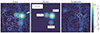 |
Fig. 1. Continuum source modeling. Left: MUSE r-band map overlayed with the 2σ and 5σ isophotes (pink) of extended Lyα emission associated with the system (Herwig et al. 2024). Shown is a cut-out of size 11″ × 11″. Middle: Best-fitting Moffat model of the continuum sources. Pink circles indicate the apertures used for spectral extraction (Fig. 2). Right: Residual flux density after subtracting the model. The crosses show the centroid position of subtracted sources. The pink circle indicates the aperture used to calculate the maximum apparent magnitude of an interloping galaxy (if any). The white cross shows the position of the spectrum used to evaluate the amount of CCD gap contamination (Appendix E). |
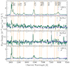 |
Fig. 2. One-dimensional spectra for the candidate quadruple AGN system. QSO1 and QSO2 are the two SDSS quasars, while AGNc1 and AGNc2 are the two additional AGN candidates. For each source, we indicate both the data and noise spectrum (see legend). Orange dashed vertical lines indicate the location of important rest-frame UV transitions at the redshift of each object obtained from a fit to the C III]λ1908 line. The location of sky-lines with residuals in the spectrum of AGNc2 are indicated with shaded vertical areas. Due to the vastly different magnitudes of the objects, the y-axis range is different in each panel. |
Quasar and AGN candidate properties and the distances between the candidates.
We fit the spectra as described in Appendix B and summarize the resulting line fluxes, widths, and upper flux limits in Table B.1. The line width of AGNc2 is narrow with ![Mathematical equation: $ \mathrm{FWHM_{CIII]}} = 600^{+80}_{-70} $](/articles/aa/full_html/2025/02/aa52452-24/aa52452-24-eq1.gif) km s−1 and consistent with a type 2 AGN, while the spectrum of AGNc1 is dominated by broad lines of
km s−1 and consistent with a type 2 AGN, while the spectrum of AGNc1 is dominated by broad lines of ![Mathematical equation: $ \mathrm{FWHM_{CIII]}} = 5040^{+1390}_{-3790} $](/articles/aa/full_html/2025/02/aa52452-24/aa52452-24-eq2.gif) km s−1, indicative of a type 1 AGN.
km s−1, indicative of a type 1 AGN.
3.2. Properties of QSO1 and QSO2
Using the fitting results (Appendix B), we could derive additional properties for the brighter SDSS quasars QSO1 and QSO2. We calculated the black hole masses using the relation and absolute accuracy estimate derived for C IV λ1550 in Vestergaard & Peterson (2006) and obtained log MBH, QSO1 = (8.3 ± 0.56) M⊙ and log MBH, QSO2 = (8.8 ± 0.56) M⊙. At the position of QSO1, radio emission is detected with a flux density of f3 GHz = (0.7 ± 0.1) mJy beam−1 in VLASS (Lacy et al. 2020) and f1.4 GHz = (1.02 ± 0.15) mJy beam−1 in VLA FIRST (Becker et al. 1994), leading to a radio slope of α = −0.49 (fν ∝ να). In addition, using the UV continuum slope from the fit to the spectrum of QSO1 (Appendix B) of β = −1.04 (fλ ∝ λβ), we calculated the ratio R = fν,5 GHz/f4400 Å (Kellermann et al. 1989) by extrapolating the rest-frame flux densities and obtained R = 3078, classifying QSO1 as radio-loud. Although no additional radio emission is detected, we cannot exclude that AGNc1 and AGNc2 are radio-loud due to the shallow survey depths2 and their dim UV continuum.
3.3. Emission line diagnostics
A commonly adopted diagnostic diagram to distinguish AGNs from star forming galaxies (SFGs) in rest-frame UV uses the line ratios C IV λ1550/C III]λ1908 (C43), which is mainly influenced by the ionization parameter, and C III]λ1908/He II λ1640 (C3He2), which is sensitive to metallicity and allows for distinction between shocks and AGN photoionization (Feltre et al. 2016). Hirschmann et al. (2019) propose demarcation lines to distinguish between active and inactive galaxies, but the current models are not capable of fully reproducing observed line ratios, and thus this would lead to large impurities in the selection of AGNs, specifically faint AGNs. Classification is further complicated because certain types of galaxies would not appear in such a diagnostic diagram: high-z radio galaxies (HzRGs) commonly have no detection of C IV λ1550 (56% in De Breuck et al. 2000), and SFGs usually show C IV λ1550 and Si IV λ1398 in absorption instead of emission (e.g., Shapley et al. 2003; Calabrò et al. 2022). In Fig. 3, we show the line ratios of the candidate AGNs and SDSS quasars together with line ratios of SFGs and different types of AGNs from the literature. The quasars and AGN candidates as well as 30% of the literature AGNs fall within the composite region of the diagram, indicating contribution from both star formation and AGN activity. Surprisingly, the line ratios of QSO1 indicate the highest contribution from star formation of all four objects, although it is definitively classified as quasar, further highlighting the difficulty in AGN selection based on UV line ratios. Also notable is that the stacks of observed SFGs selected based on C III]λ1908 emission are classified as composite objects as well.
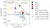 |
Fig. 3. Diagnostic diagram based on the line ratios C IV λ1550/C III]λ1908 and C III]λ1908/He II λ1640. Demarcation lines between AGN, SFGs, and composite line ratios are taken from Hirschmann et al. (2019). The values for QSO1, AGNc1, AGNc2, and QSO2 are compared to literature values for different types of galaxies: C III]λ1908-selected SFGs at z > 2.9 binned by stellar mass (Llerena et al. 2022), high-z radio galaxies with detections in all lines (De Breuck et al. 2000; Matsuoka et al. 2009), high-z X-ray selected type 2 quasars (Nagao et al. 2006), and local Seyfert 2 AGNs (Nagao et al. 2006). |
However, the detection of N V λ1240 and Si IV λ1398, two highly ionized lines, and the extreme line width of AGNc1, which is larger than 5000 km s−1, firmly point toward an AGN origin. If these broad lines were produced by galactic-scale outflows instead, the violent kinematics should lead to a high contribution from shocks and likely result in a detectable C IV λ1550 emission line. The upper limit on the equivalent width (EW) of C IV λ1550 lies above the AGN demarcation line of ≲ 3 Å at the corresponding C IV λ1550/He II λ1640 ratio limit for AGNc1 of < 1 (Nakajima et al. 2018), and AGN ionization can therefore not be excluded based on the non-detection of the line. The ratio of Si IV λ1398 to He II λ1640 exceeds what is typical for HzRGs (Humphrey et al. 2008) as well as quasars (Nagao et al. 2006). On the other hand, the C IV λ1550 EW of AGNc2 lies firmly above the demarcation line of 12 Å in Nakajima et al. (2018) at the corresponding C IV λ1550/He II λ1640 ratio for AGNc2, indicating that this source is an AGN.
4. Discussion
4.1. Clues from the peculiar extended Lyα emission
The pink contours in Fig. 1 show the 2σ and 5σ levels of extended Lyα emission, corresponding to a surface brightness of 3.0 × 10⁻¹⁸ erg s−1 cm−2 arcsec−2 and 7.4 × 10⁻¹⁸ erg s−1 cm−2 arcsec−2, respectively, and determined after subtracting the empirical quasar point spread functions and continuum sources from the combined cube. This analysis is described in detail in Herwig et al. (2024) and González Lobos et al. (2023). The nebular emission extends for about 50 kpc in the southeast direction with respect to QSO1, starting from the projected location of AGNc2. Additional Lyα emission coincides with the position of AGNc1. Surprisingly, the surface brightness level of the extended Lyα emission is much lower than typically found for multiple AGN systems (Hennawi et al. 2015; Arrigoni Battaia et al. 2018), and the AGN candidates are not embedded in the nebula. Instead, the flux-weighted centroid of the extended emission is offset from QSO1 by 34 kpc (Herwig et al. 2024). Possible explanations for this could be a faster evolution and therefore early cool gas depletion of outlier density peaks in the Universe or a later merger stage of the close AGN triplet candidate presented in this work. Moreover, strong feedback effects might have already depleted the circumgalactic medium of this system of cool gas.
The peculiar morphology of the extended Lyα emission could be further evidence of violent, ongoing galaxy interactions. If the interstellar medium of AGNc2 is ram-pressure stripped during the infall into the hot halo of QSO1, the trailing dense gas behind AGNc2 could become visible as extended Lyα emission. Indeed, estimating the stripped gas mass yields a lower limit of at least 6.3 × 10⁹ M⊙ when assuming the line-of-sight velocity or roughly 8.6 × 10⁹ M⊙ when using a conservative estimate of the 3D velocity, while the estimated cool gas mass visible as extended Lyα emission amounts to roughly 4.8 × 10⁹ M⊙ (Appendix C). This first estimate confirms that ram-pressure stripping could be an effective mechanism in this configuration and could indeed explain the peculiar appearance of the extended Lyα emission. Evidence for similar ram-pressure stripping events around high-z quasars have been recently invoked by other studies on extended Lya emission (e.g., Chen et al. 2021).
4.2. Evolutionary scenario
The close separation of QSO1, AGNc1, and AGNc2 and evidence for gas stripping and therefore ongoing galaxy interactions makes it very likely that the host galaxies will quickly merge into one massive galaxy. The result of such a merger is predicted to have a host halo mass of 1013 M⊙ (Bhowmick et al. 2020). Three-body interactions have a high likelihood of ejecting one of the participants via gravitational recoil (Partmann et al. 2024). This is the most probable evolution of the close black hole system, although two or even three mergers are also possible and would lead to the emission of gravitational waves possibly contributing to the gravitational wave background (Sesana et al. 2008) and likely the formation of an ultra-massive (MBH > 1010 M⊙) black hole. However, ejection or stalling of one or two black holes is predicted to not hinder fast growth. In simulations, the strong gravitational forces lead to quick infall times of gas into the most massive black hole and facilitate black hole mass growth up to 1010 M⊙ irrespective of coalescence (Hoffman et al. 2023). The extreme density peak implied by the presence of four AGNs in close proximity and three AGNs in the same dark matter halo is likely accompanied by a galaxy overdensity. This hypothesis needs to be tested by multi-wavelength observations targeting the galaxy population on megaparsec scales around the quadruple AGN candidate. If confirmed, the most probable evolutionary path of this extraordinary system is the formation of a galaxy cluster in which the brightest cluster galaxy is formed out of the close triple AGN host galaxies.
4.3. Incidence rate of AGN multiplets
Following Hennawi et al. (2015), an estimate of the probability of finding two close-companion AGNs of a known quasar can be obtained from the two-point correlation function for quasars, and for a magnitude limit of 25 mag, it amounts to ∼10−8, or ∼10−5 if considering any halo-scale triple AGN (Appendix D). A different generalized estimate for the AGN multiplet incidence rate can be obtained by considering the full observed parent sample. Including the candidate presented in this work, two AGN multiplets have been identified within the QSO MUSEUM survey encompassing 134 quasars at 3 < z < 4 observed with MUSE to similar depths (Arrigoni Battaia et al. 2019; Herwig et al. 2024; González Lobos et al., in preparation). This corresponds to an incidence rate for such systems of 1.5 % with Poisson errors for small-number statistics from Gehrels (1986). This value is much larger than the above calculations and larger than previously believed (Hennawi et al. 2015). It implies
  undiscovered multiplet systems around SDSS quasars (Pâris et al. 2018) in the same redshift range (with a median redshift of z = 3.226), and when extrapolated to the entire sky, this value indicates that there could be
  AGN multiplets. Assuming that black hole multiplets populate the massive end of the halo mass function and that 65% of them are visible as AGN multiplets (Hoffman et al. 2023), this number would amount to all halos with masses above Mvir = (5 ± 1)×1013 M⊙ of the z = 3.226 halo mass function (Behroozi et al. 2013).
5. Summary
We have presented an unlensed candidate quadruple AGN system at z ∼ 3 consisting of two SDSS type 1 quasars at a separation of roughly 480 kpc (QSO1 and QSO2) and two AGN candidates (AGNc1 and AGNc2) accompanying QSO1 in close proximity with a projected separation of up to 20 kpc. The identification as probable AGN candidates is based on C43 versus C4He2 line ratios; high ionization lines, such as N V λ1240 in their spectrum; and emission line widths. AGNc1 is a potential type 1 AGN, while the spectral characteristics of AGNc2 align with those of a type 2 quasar. Further observations in X-ray or of rest-frame optical lines can confirm these objects as AGNs and allow for more reliable redshift determination.
The close triple system (QSO1, AGNc1, AGNc2) is associated with a Lyα nebula, although it is not embedded within it. A possible explanation for the presence of peculiar Lyα-bright gas is ram-pressure stripping of AGNc2 during its infall into the halo of QSO1. This extraordinary system likely pinpoints a site of galaxy cluster formation. This hypothesis needs to be tested further by studying the megaparsec-scale galaxy overdensity surrounding the quadruple AGN candidate.
This new candidate quadruple AGN allowed us to refine the incidence rate of such rare systems around z ∼ 3 SDSS quasars to be 1.5 %. Pre-selection of SDSS quasars with close faint sources (e.g., Euclid) is essential to building the statistical sample (12 systems) needed to confirm our statistics and constrain current models (e.g., Hoffman et al. 2023). Without it, additional
  MUSE observations (1 hour per source) of SDSS quasars would be required.
In this smaller aperture, the magnitude of QSO1 decreases to mQSO1 = (22.34 ± 0.09) mag.
The VLASS continuum image rms is 70 μJy/beam (Lacy et al. 2020), and the FIRST data have an rms of 149 μJy/beam close to the system location (Becker et al. 1994).
Generated with the "The Cerro Paranal Advanced Sky Model", https://www.eso.org/observing/etc/doc/skycalc/The_Cerro_Paranal_Advanced_Sky_Model.pdf
Acknowledgments
We thank the anonymous referee for their constructive comments that helped improve the manuscript and Guinevere Kauffmann for providing useful comments to an earlier version of this work. E.P.F. is supported by the international Gemini Observatory, a program of NSF NOIRLab, which is managed by the Association of Universities for Research in Astronomy (AURA) under a cooperative agreement with the U.S. National Science Foundation, on behalf of the Gemini partnership of Argentina, Brazil, Canada, Chile, the Republic of Korea, and the United States of America.
References
- Abdurro’uf, Accetta, K., Aerts, C., et al. 2022, ApJS, 259, 35 [NASA ADS] [CrossRef] [Google Scholar]
- Agnello, A., Lin, H., Kuropatkin, N., et al. 2018, MNRAS, 479, 4345 [Google Scholar]
- Arrigoni Battaia, F., Prochaska, J. X., Hennawi, J. F., et al. 2018, MNRAS, 473, 3907 [NASA ADS] [CrossRef] [Google Scholar]
- Arrigoni Battaia, F., Hennawi, J. F., Prochaska, J. X., et al. 2019, MNRAS, 482, 3162 [NASA ADS] [CrossRef] [Google Scholar]
- Arrigoni Battaia, F., Chen, C.-C., Liu, H.-Y. B., et al. 2022, ApJ, 930, 72 [NASA ADS] [CrossRef] [Google Scholar]
- Assef, R. J., Stern, D., Noirot, G., et al. 2018, ApJS, 234, 23 [Google Scholar]
- Bacon, R., Accardo, M., Adjali, L., et al. 2010, in Ground-based and Airborne Instrumentation for Astronomy III, eds. I. S. McLean, S. K. Ramsay, & H. Takami, Society of Photo-Optical Instrumentation Engineers (SPIE) Conference Series, 7735, 773508 [Google Scholar]
- Becker, R. H., White, R. L., & Helfand, D. J. 1994, in Astronomical Data Analysis Software and Systems III, eds. D. R. Crabtree, R. J. Hanisch, & J. Barnes, Astronomical Society of the Pacific Conference Series, 61, 165 [NASA ADS] [Google Scholar]
- Behroozi, P. S., Wechsler, R. H., & Conroy, C. 2013, ApJ, 770, 57 [NASA ADS] [CrossRef] [Google Scholar]
- Bhowmick, A. K., Di Matteo, T., & Myers, A. D. 2020, MNRAS, 492, 5620 [NASA ADS] [CrossRef] [Google Scholar]
- Calabrò, A., Pentericci, L., Talia, M., et al. 2022, A&A, 667, A117 [NASA ADS] [CrossRef] [EDP Sciences] [Google Scholar]
- Chen, C.-C., Arrigoni Battaia, F., Emonts, B. H. C., Lehnert, M. D., & Prochaska, J. X. 2021, ApJ, 923, 200 [NASA ADS] [CrossRef] [Google Scholar]
- De Breuck, C., Röttgering, H., Miley, G., van Breugel, W., & Best, P. 2000, A&A, 362, 519 [Google Scholar]
- Djorgovski, S. G., Courbin, F., Meylan, G., et al. 2007, ApJ, 662, L1 [NASA ADS] [CrossRef] [Google Scholar]
- Dullo, B. T., Graham, A. W., & Knapen, J. H. 2017, MNRAS, 471, 2321 [NASA ADS] [CrossRef] [Google Scholar]
- Farina, E. P., Montuori, C., Decarli, R., & Fumagalli, M. 2013, MNRAS, 431, 1019 [NASA ADS] [CrossRef] [Google Scholar]
- Farina, E. P., Arrigoni-Battaia, F., Costa, T., et al. 2019, ApJ, 887, 196 [Google Scholar]
- Feltre, A., Charlot, S., & Gutkin, J. 2016, MNRAS, 456, 3354 [Google Scholar]
- Fossati, M., Fumagalli, M., Lofthouse, E. K., et al. 2021, MNRAS, 503, 3044 [NASA ADS] [CrossRef] [Google Scholar]
- Fukugita, M., Nakamura, O., Schneider, D. P., Doi, M., & Kashikawa, N. 2004, ApJ, 603, L65 [CrossRef] [Google Scholar]
- García-Vergara, C., Rybak, M., Hodge, J., et al. 2022, ApJ, 927, 65 [CrossRef] [Google Scholar]
- Gehrels, N. 1986, ApJ, 303, 336 [Google Scholar]
- González Lobos, V., Arrigoni Battaia, F., Chang, S.-J., et al. 2023, A&A, 679, A41 [NASA ADS] [CrossRef] [EDP Sciences] [Google Scholar]
- Green, P. J., Myers, A. D., Barkhouse, W. A., et al. 2011, ApJ, 743, 81 [NASA ADS] [CrossRef] [Google Scholar]
- Gunn, J. E., Gott, J., & Richard, I. 1972, ApJ, 176, 1 [Google Scholar]
- Guo, H., Shen, Y., & Wang, S. 2018, Astrophysics Source Code Library [record ascl:1809.008] [Google Scholar]
- Habouzit, M., Volonteri, M., Somerville, R. S., et al. 2019, MNRAS, 489, 1206 [CrossRef] [Google Scholar]
- Hennawi, J. F., Strauss, M. A., Oguri, M., et al. 2006, AJ, 131, 1 [Google Scholar]
- Hennawi, J. F., Prochaska, J. X., Cantalupo, S., & Arrigoni-Battaia, F. 2015, Science, 348, 779 [Google Scholar]
- Herwig, E., Arrigoni Battaia, F., González Lobos, J., et al. 2024, A&A, 691, A210 [NASA ADS] [CrossRef] [EDP Sciences] [Google Scholar]
- Hirschmann, M., Charlot, S., Feltre, A., et al. 2019, MNRAS, 487, 333 [NASA ADS] [CrossRef] [Google Scholar]
- Hoffman, C., Chen, N., Di Matteo, T., et al. 2023, MNRAS, 524, 1987 [Google Scholar]
- Humphrey, A., Villar-Martín, M., Vernet, J., et al. 2008, MNRAS, 383, 11 [NASA ADS] [CrossRef] [Google Scholar]
- Husband, K., Bremer, M. N., Stanway, E. R., et al. 2013, MNRAS, 432, 2869 [NASA ADS] [CrossRef] [Google Scholar]
- Kalfountzou, E., Santos Lleo, M., & Trichas, M. 2017, ApJ, 851, L15 [NASA ADS] [CrossRef] [Google Scholar]
- Kayo, I., & Oguri, M. 2012, MNRAS, 424, 1363 [NASA ADS] [CrossRef] [Google Scholar]
- Kellermann, K. I., Sramek, R., Schmidt, M., Shaffer, D. B., & Green, R. 1989, AJ, 98, 1195 [Google Scholar]
- Kocevski, D. D., Barro, G., McGrath, E. J., et al. 2023, ApJ, 946, L14 [NASA ADS] [CrossRef] [Google Scholar]
- Lacy, M., Baum, S. A., Chandler, C. J., et al. 2020, PASP, 132, 035001 [Google Scholar]
- Lau, M. W., Prochaska, J. X., & Hennawi, J. F. 2016, ApJS, 226, 25 [NASA ADS] [CrossRef] [Google Scholar]
- Liu, X., Shen, Y., & Strauss, M. A. 2011, ApJ, 736, L7 [Google Scholar]
- Llerena, M., Amorín, R., Cullen, F., et al. 2022, A&A, 659, A16 [NASA ADS] [CrossRef] [EDP Sciences] [Google Scholar]
- Matsuoka, K., Nagao, T., Maiolino, R., Marconi, A., & Taniguchi, Y. 2009, A&A, 503, 721 [NASA ADS] [CrossRef] [EDP Sciences] [Google Scholar]
- Mehrgan, K., Thomas, J., Saglia, R., et al. 2019, ApJ, 887, 195 [NASA ADS] [CrossRef] [Google Scholar]
- Nagao, T., Maiolino, R., & Marconi, A. 2006, A&A, 447, 863 [NASA ADS] [CrossRef] [EDP Sciences] [Google Scholar]
- Nakajima, K., Schaerer, D., Le Fèvre, O., et al. 2018, A&A, 612, A94 [NASA ADS] [CrossRef] [EDP Sciences] [Google Scholar]
- Nigoche-Netro, A., Aguerri, J. A. L., Lagos, P., et al. 2010, A&A, 516, A96 [NASA ADS] [CrossRef] [EDP Sciences] [Google Scholar]
- Onoue, M., Kashikawa, N., Uchiyama, H., et al. 2018, PASJ, 70, S31 [NASA ADS] [CrossRef] [Google Scholar]
- Overzier, R. A. 2016, A&ARv, 24, 14 [Google Scholar]
- Pâris, I., Petitjean, P., Ross, N. P., et al. 2017, A&A, 597, A79 [NASA ADS] [CrossRef] [EDP Sciences] [Google Scholar]
- Pâris, I., Petitjean, P., Aubourg, É., et al. 2018, A&A, 613, A51 [Google Scholar]
- Partmann, C., Naab, T., Rantala, A., et al. 2024, MNRAS, 532, 4681 [NASA ADS] [CrossRef] [Google Scholar]
- Pfeifle, R. W., Satyapal, S., Manzano-King, C., et al. 2019, ApJ, 883, 167 [Google Scholar]
- Planck Collaboration VI. 2020, A&A, 641, A6 [NASA ADS] [CrossRef] [EDP Sciences] [Google Scholar]
- Runnoe, J. C., Brotherton, M. S., & Shang, Z. 2012, MNRAS, 422, 478 [Google Scholar]
- Sandrinelli, A., Falomo, R., Treves, A., Scarpa, R., & Uslenghi, M. 2018, MNRAS, 474, 4925 [NASA ADS] [CrossRef] [Google Scholar]
- Sesana, A., Vecchio, A., & Colacino, C. N. 2008, MNRAS, 390, 192 [NASA ADS] [CrossRef] [Google Scholar]
- Shapley, A. E., Steidel, C. C., Pettini, M., & Adelberger, K. L. 2003, ApJ, 588, 65 [Google Scholar]
- Shen, Y., Hall, P. B., Horne, K., et al. 2019, ApJS, 241, 34 [NASA ADS] [CrossRef] [Google Scholar]
- Shen, X., Hopkins, P. F., Faucher-Giguère, C.-A., et al. 2020, MNRAS, 495, 3252 [Google Scholar]
- Soto, K. T., Lilly, S. J., Bacon, R., Richard, J., & Conseil, S. 2016, MNRAS, 458, 3210 [Google Scholar]
- Trainor, R. F., & Steidel, C. C. 2012, ApJ, 752, 39 [NASA ADS] [CrossRef] [Google Scholar]
- Uchiyama, H., Toshikawa, J., Kashikawa, N., et al. 2018, PASJ, 70, S32 [NASA ADS] [CrossRef] [Google Scholar]
- Vestergaard, M., & Peterson, B. M. 2006, ApJ, 641, 689 [Google Scholar]
- Virtanen, P., Gommers, R., Oliphant, T. E., et al. 2020, Nat. Methods, 17, 261 [Google Scholar]
- Ward, E., de la Vega, A., Mobasher, B., et al. 2024, ApJ, 962, 176 [NASA ADS] [CrossRef] [Google Scholar]
- Weilbacher, P. M., Streicher, O., Urrutia, T., et al. 2014, in Astronomical Data Analysis Software and Systems XXIII, ed. N. Manset& P. Forshay, Astronomical Society of the Pacific Conference Series, 485, 451 [NASA ADS] [Google Scholar]
- Weilbacher, P. M., Streicher, O., & Palsa, R. 2016, Astrophysics Source Code Library [record ascl:1610.004] [Google Scholar]
- Weilbacher, P. M., Palsa, R., Streicher, O., et al. 2020, A&A, 641, A28 [NASA ADS] [CrossRef] [EDP Sciences] [Google Scholar]
- White, M., Myers, A. D., Ross, N. P., et al. 2012, MNRAS, 424, 933 [NASA ADS] [CrossRef] [Google Scholar]
- Wijers, N. A., & Schaye, J. 2022, MNRAS, 514, 5214 [NASA ADS] [CrossRef] [Google Scholar]
Appendix A: Rejecting the possibility of gravitational lensing
A possible explanation for multiple quasars in close separation is gravitational lensing of a single source (e.g., Agnello et al. 2018). In this case, the spectra would be very similar with slight variations due to different light paths. While all AGN in this system appear to have significantly different spectra (Fig. 2), this view might be skewed by the low signal to noise ratio of the fainter objects. While AGNc2 is a type 2 AGN candidate as it only shows narrow emission lines and should therefore be viewed at an entirely different angle than QSO1 and AGNc1, we explore the possibility that the latter two objects are actually two lensed images of the same quasar.
In this case, we expect to find a massive object capable of acting as the gravitational lens in between the two images. To calculate the necessary magnitude of a lensing elliptical galaxy, we followed Farina et al. (2013), making use of the Faber–Jackson relation by Nigoche-Netro et al. (2010) and assuming an isothermal sphere to link mass and velocity dispersion. Assuming an Einstein ring radius of Θ = 1.05″, corresponding to half of the angular distance between QSO1 and AGNc1, the minimal possible apparent r-band magnitude of an interloper galaxy is m = 21.6 at z ≈ 1.89, brighter than both the AGN candidates and QSO1.
We then inspected the residuals of the point spread function modeling (Fig. 1, right). There, an artifact of the CCD gap becomes apparent as vertical line, but no foreground galaxy is revealed. The r-band magnitude in a 1.6″ aperture between QSO1 and AGNc1 (indicated as pink circle in Fig. 1, right) after masking negative values potentially arising due to the model subtraction is 26.4 mag, far below the faintest possible lensing galaxy. Therefore we conclude that no lensing geometry fits the observed pattern without revealing the lensing galaxy in the data cube.
Appendix B: Spectral fitting
We attempted to fit a set of rest-frame UV lines to the spectra of all four sources presented in Fig. 2, namely Lyα, N V λ1240, Si IV λ1398, C IV λ1550, He II λ1640 and C III]λ1908. Due to the stark difference in magnitude and therefore data quality, we adopted two different methods. All line fluxes, EWs, and line widths are summarized in Table B.1.
Line fluxes, equivalent widths, and line width.
B.1. SDSS QSOs
The two SDSS detected quasars QSO1 and QSO2 have sufficient S/N to be fitted using the package pyQSOFIT (Guo et al. 2018; Shen et al. 2019). We used the spectrum extracted from the MUSE cube as explained in Sec. 3.1 for QSO1 as it has higher S/N than the SDSS spectrum. For QSO2, only the SDSS spectrum is available. Errors were estimated through 250 MCMC samplings, and the line width FWHMCIII] was determined from the fit to the C III]λ1908 line. The Gaussian model used to describe the C III]λ1908 line is affected by the Gaussian smoothing kernel applied before fitting, and we thus corrected the values down to reflect the intrinsic line width. Although we attempted to include a component for the N V λ1240 and Si IV λ1398 line when fitting QSO2, we did not find a combination of priors that leads to convergence and we thus do not report fluxes for these lines. From pyQSOFIT we also obtained the continuum luminosity L(1350 Å) and the FWHM of C IV λ1550 and used them to calculate black hole mass estimates for QSO1 and QSO2 using the relation and absolute accuracy estimate derived in Vestergaard & Peterson (2006). With L(1350 Å)QSO1 = 1044.91±0.01 erg s−1, L(1350 Å)QSO2 = 1045.32±0.02 erg s−1, FWHMCIV, QSO1 = (3610 ± 20) km s−1 and FWHMCIV, QSO2 = (5350 ± 260) km s−1, we obtained the values log MBH, QSO1 = (8.3 ± 0.56) M⊙ and log MBH, QSO2 = (8.8 ± 0.56) M⊙.
B.2. AGN candidates
Due to low S/N, the spectra of candidates AGNc1 and AGNc2 cannot be fitted with pyQSOFIT and we instead subtracted a constant local continuum value before fitting emission lines using the function curve_fit in scipy (Virtanen et al. 2020).
In particular, we obtained a first estimate of the line widths σini by calculating the second moment of the Lyα line (AGNc1) and C IV λ1550 line (AGNc2) in an unsmoothed spectrum. We used the resulting values of  km s−1 and
  km s−1 respectively (corresponding to
  and
and  respectively) to constrain the following fit.
Then, we calculated the continuum level and its variance by masking all shaded gray areas in Fig. 2 as well as marked emission lines within ±3σini (AGNc1) and ±5σini (AGNc2) of the systemic wavelength. The chosen masking windows are large enough to ensure no line emission is contaminating the continuum calculation and small enough to retain local continuum around each fitted line. The latter is particularly important for the broad line width of AGNc1. Due to the large velocity shift of C IV λ1550 in AGNc2, we adjusted the wavelength of the line downward by 10 Å to ensure appropriate masking and fitting. For each fitted emission line, we then considered the next 40 unmasked wavelength channels (corresponding to 50 Å) left and right of the expected peak λsys and calculated the 25th, 50th, and 75th percentile to get the median continuum value (Cont50) and typical range (Cont25, Cont75). Cont25 is consistent with the noise level for most lines (Fig. B.1, B.2) and thus represents a conservative lower limit for the continuum level as the AGN candidates are detected in continuum emission (Fig. 1). As the determination of the continuum introduces the largest uncertainty in the fit, in particular for the broad lines of AGNc1, we performed three emission line fittings using each of these continuum values for the subtraction and derived conservative line flux errors from the difference in results.
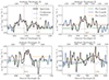 |
Fig. B.1. Gaussian fit to the emission lines after subtraction of the three different continua (Cont25, Cont50, Cont75) from the spectrum of AGNc1, smoothed by a 1D Gaussian kernel with σ = 3 pixels. The vertical dotted brown line indicates the expected wavelength λsys of the respective emission line, highlighting that the redshift determined from the peak of the C III]λ1908 line complex could be overestimated and the He II λ1640 line might be misidentified. Blue spectral regions mark the 50 Å windows used to calculate the continuum. |
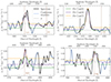 |
Fig. B.2. Same as Fig. B.1 but for AGNc2. The C IV λ1550 line peak of the fit is blueshifted with respect to zCIII] by −2208 km s−1. The shaded gray strip indicates the masked area affected by sky emission. |
During line fitting, we assumed a single Gaussian model within the bounds given in Table B.2, and weighted the fit with noise spectra extracted from the rescaled variance cube. The Lyα and N V λ1240 line of AGNc1 are likely blended together and are thus fitted together using two Gaussian lines centered on the respective systemic wavelengths. From the Gaussian model of the C III]λ1908 line, we obtained the line width FWHMCIII] of  km s−1 (AGNc1) and
  km s−1 (AGNc2). These values are larger than the calculation of the second moment in unsmoothed spectra, but are consistent with line widths in type 1 AGNs and type 2 AGNs respectively. We again corrected the line width of the Gaussian model by the smoothing kernel.
Bounds of the Gaussian fitting model.
If the flux value of an emission line is consistent with zero after subtracting Cont75, we consider it as undetected and only place upper limits on the flux. This is the case for C IV λ1550 (AGNc1) and N V λ1240 and Si IV λ1398 (AGNc2). We derived upper limits from the channel-wise RMS of the spectra scaled to 2.355σini and report the limit at 3σ significance.
We derived EWs and uncertainties for the high ionization lines Si IV λ1398 and C IV λ1550 from the three different Gaussian line fittings and their respective continuum levels and derived upper limits on EWs by assuming the median continuum level Cont50 and the upper flux limit.
Appendix C: Estimating the efficiency of ram pressure stripping
The peculiar extended Lyα emission associated with the close triple system might be a further indication of on-going galaxy interaction as the emission could be a result of ram-pressure stripped interstellar medium of AGNc2 appearing Lyα bright. This could further explain the large velocity differences in the nebula obtained from the first moment with respect to AGNc2 (Fig. C.1), reaching 1500 km s−1 at the East edge of the isophote furthest away from the AGN candidate and generally approaching the systemic redshift of AGNc2 closer to it, although the nebula shows significant turbulence. To determine the feasibility of this hypothesis, we estimated the efficiency of stripping in the configuration of the system.
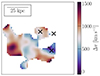 |
Fig. C.1. Moment 1 of the extended Lyα emission with respect to the systemic redshift of AGNc2. The centroid positions of QSO1, AGNc1 and AGNc2 are indicated with black crosses. |
Ram-pressure stripping is possible if ρhalovAGNc22 > 2πGσsσg (Gunn et al. 1972). In this, ρhalo is the density of the hot gas in the halo of QSO1 and obtained from the typical volume-weighted number density in a hot halo of mass log(M/M⊙) = 12.5 − 13 at 20 % of the virial radius corresponding to the projected distance of AGNc2, log(n/[cm−3]) = −3.9 (Wijers & Schaye 2022). This mass bin is chosen as it includes the halo mass estimate for single quasars at this redshift (1012.5 M⊙) as well as threefold this mass (1013 M⊙) in case QSO1, AGNc1 and AGNc2 all share one dark matter halo and all three resided in quasar-typical massive halos before. This larger halo mass is also similar to that estimated for one of the known triplets (Arrigoni Battaia et al. 2022). vAGNc2 is the velocity with which AGNc2 is crossing the halo of QSO1 and at least as high as the line-of-sight velocity reported in Table 1. A conservative estimate of the 3D velocity is  km s−1.
The gravitational pull of AGNc2 withstanding the ram pressure is described by the stellar and gas surface densities σs and σg. AGN hosts at z ∼ 3 typically have a massive (M⋆ ∼ 1011M⊙), compact stellar component described by a Sersic profile with an average Sersic index of 2.6 and an effective radius of 0.9 kpc (Kocevski et al. 2023). The gas disk is well-described by an exponential profile, and we assumed an effective radius of 2 kpc (Ward et al. 2024) and a cold gas mass fraction of 20 %. The stripped gas mass can then be estimated by integrating the gas mass profile beyond the radius at which ram pressure exceeds the gravitational pull of the galaxy, and it amounts to at least 6.3 × 10⁹M⊙ when assuming the line-of-sight velocity, or roughly 8.6 × 10⁹M⊙ when using the 3D velocity.
To contrast this with the Lyα-bright gas, we estimated the mass from the extended emission using the equation Mcool ∼ ANHmp/X with the Lyα nebula area A = 1437 kpc2 (Herwig et al. 2024), the proton mass mp and hydrogen fraction X = 0.76 and the typical column density of cool gas in the circumgalactic medium, log(NH/[cm−2]) = 20.5 (Lau et al. 2016). The latter quantity is associated with the highest uncertainty as it can vary by one order of magnitude, and it might not be applicable to extraordinary systems. With these values, we obtained an estimated cool gas mass in the Lyα nebula of 4.8 × 10⁹M⊙.
Appendix D: Probability of finding a similarly close AGN triplet
The probability to find two additional AGNs close to a known quasar can be estimated using
with the co-moving number density of AGNs nQSO, the AGN-filled volume V, the maximum distance between the AGNs rmax and the two-point correlation function of quasars ξ(r). This follows from a similar argument as presented in Hennawi et al. (2015), but we do not include the fourth object, QSO2, in the estimation as the large projected distance implies that QSO2 does not share a host halo with the other three objects (yet) and thus, other assumptions have to be made in the calculation. Specifically, in the case of a triplet, equation 2 in Hennawi et al. (2015) will only contain three permutations for the two-point correlation function and one permutation for the three-point correlation function. Although the three-point correlation function relates to ξ as  (Hennawi et al. 2015), in our order-of-magnitude estimation, we can approximate ζ ∼ ξ, hence the factor of four in the above probability equation.
We inferred nQSO from the quasar luminosity function at z = 3 (Shen et al. 2020) with a lower magnitude limit of mmin,1450 Å = 25 mag and the quasar bolometric luminosity correction from Runnoe et al. (2012) resulting in nQSO = 9.3 × 10⁻⁵cMpc−3. Due to the imprecision in redshift determinations from broad QSO emission lines and the possibility of high peculiar velocities causing additional Doppler shifts, we extrapolated the maximum distance in the triplet, rmax, as the highest projected distance plus a 50 % margin to account for projection effects. This yields a quasar-filled comoving volume of V = 8 × 10⁻³ cMpc3. On small scales, the two-point correlation function is well described with  with γ = 2 and r0 = 5.4 ± 0.3h−1 cMpc (Kayo & Oguri 2012). Plugging in these values, we obtained P ≈ 3 × 10⁻⁸.
The candidate triple AGN presented in this work is closer than previously found AGN triples. To get an estimate of the probability to find any AGN triple on halo scales, we repeated the calculation using rmax = 150 kpc, corresponding roughly to the virial radius of a halo with mass 1013 M⊙, and obtained a probability of P ≈ 2 × 10⁻⁵. In contrast, the probability Pr to find three AGNs with rmax = 30 kpc at random without considering clustering can be described with Pr = nQSO2 × V2 (Hennawi et al. 2015) and would be exceedingly rare with Pr = 5.5 × 10⁻¹³.
Appendix E: Examining possible sources of spectral contamination
Multiple sources of artifacts and spurious signal can contaminate observational data. Here, we examine a few of these effects and determine the level of contamination introduced.
The first artifact to consider is residual emission from the CCD gap visible in the continuum image after subtraction of QSO1, AGNc1 and AGNc2 (Fig. 1, right panel). In particular, the spectrum of AGNc2 overlaps with the CCD gap. Thus, we extracted a spectrum at the same RA as AGNc2, but close to a flux peak on the CCD gap and rescaled it to match the mean pixel value at the position of AGNc2 in the residual image. This region is indicated by a white plus in Fig. 1. The spectrum, smoothed with the same Gaussian kernel of size σ = 3 pixels, is displayed in Fig. E.1. For reference, we also show the spectrum of AGNc2 as well as the expected wavelengths of emission lines.
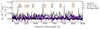 |
Fig. E.1. Check for possible sources of contamination in the spectrum of AGNc2. The spectrum taken from the region affected by CCD gap artifacts and the mean background spectrum are compared to the spectrum of AGNc2 and its expected emission line wavelengths. |
While the CCD gap might introduce a noisy contribution to the continuum, it does not show strong emission features coinciding with the fitted emission lines of AGNc2.
Next, we examined the level of background emission in the cube by visually selecting ten regions within the same aperture as the spectra with a radius of 0.8″ without continuum emission, taking the mean of the extracted spectra and smoothing it with the Gaussian kernel of size σ = 3 pixels. The obtained spectrum is also displayed in Fig. E.1 and represents the typical channel-wise background level in the data. Due to its low level, it is not expected to contribute significantly to the continuum emission in any part of the spectra.
A third source of contamination are strong atmospheric emission lines contributing significant flux peaks for the faint sources considered in this work. Despite careful subtraction of the sky spectrum in two different steps during the data reduction and before combining the individual exposures, residuals of lines can still remain in the combined data (Soto et al. 2016). These residuals appear as very thin (one to three pixel wide) emission lines in the spectrum of continuum sources if they were masked together with source emission lines during sky removal. The spectrum of AGNc2 is specifically affected by this as there are multiple narrow lines visible in the unsmoothed spectrum of the combined cube as well as the individual exposures. In Fig. E.2, we show the affected spectral windows together with a sky emission model3.
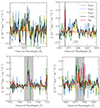 |
Fig. E.2. Unsmoothed spectra of AGNc2 extracted from the three exposures (Exp1, Exp2, Exp3, green, blue, yellow, respectively) and the combined cube (Comb, black) in spectral windows of narrow emission lines. A sky emission spectrum (Sky, red) is plotted in arbitrary flux units showing the position of atmospheric emission lines. Shaded gray areas are the same as in Fig. 2. To avoid contamination of the close-by C IV λ1550 line, the sky emission line in the top right panel is masked before smoothing. The spectral extraction region falls onto the masked CCD gap in the third exposure, leading to a lower flux. We note that we performed the median combination of the cubes pixel by pixel but summed the displayed spectra over multiple pixels. Consequently, the spectrum extracted from the median-combined cube differs from the median spectrum of those from the individual exposures. |
In these unsmoothed spectra, the difference in line width to C IV λ1550 becomes apparent. Each of the narrow emission features not assignable to a common AGN UV line coincides with the position of a sky emission line within one or two pixels. Therefore, these additional lines are most likely sky subtraction residuals.
Finally, given the small number of exposures obtained, individual data cubes could contribute significantly to emission lines, particularly if the line width is narrow. To exclude the possibility that the narrow lines in the spectrum of AGNc2 are spurious, we excluded in turn one of the three exposures during combination of the final cube and examined the Lyα and C IV λ1550 lines in the different resulting spectra in comparison to the spectrum presented in Fig. 2. As shown in Fig. E.3, the line emission persists irrespective of the combination of exposures. We caution that the gap between CCDs, which is masked before combination of the cubes, covers parts of the PSF of AGNc2 in the third exposure. However, when combining only two cubes, masked areas in one data cube are filled in with the values of the other data cube. This is the reason why the seemingly decreased line flux of exposure 3 (Fig. E.2) does not have a strong effect on the line flux in the combined cube (Fig. E.3).
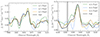 |
Fig. E.3. Smoothed spectra of AGNc2 at the wavelength of the Lyα (left) and C IV λ1550 (right) emission extracted from cubes after combining only two of the three exposures as well as the full cube. The shaded gray area is the same as in Fig. 2 and masked before smoothing. |
All Tables
All Figures
|
Fig. 1. Continuum source modeling. Left: MUSE r-band map overlayed with the 2σ and 5σ isophotes (pink) of extended Lyα emission associated with the system (Herwig et al. 2024). Shown is a cut-out of size 11″ × 11″. Middle: Best-fitting Moffat model of the continuum sources. Pink circles indicate the apertures used for spectral extraction (Fig. 2). Right: Residual flux density after subtracting the model. The crosses show the centroid position of subtracted sources. The pink circle indicates the aperture used to calculate the maximum apparent magnitude of an interloping galaxy (if any). The white cross shows the position of the spectrum used to evaluate the amount of CCD gap contamination (Appendix E). |
| In the text | |
|
Fig. 2. One-dimensional spectra for the candidate quadruple AGN system. QSO1 and QSO2 are the two SDSS quasars, while AGNc1 and AGNc2 are the two additional AGN candidates. For each source, we indicate both the data and noise spectrum (see legend). Orange dashed vertical lines indicate the location of important rest-frame UV transitions at the redshift of each object obtained from a fit to the C III]λ1908 line. The location of sky-lines with residuals in the spectrum of AGNc2 are indicated with shaded vertical areas. Due to the vastly different magnitudes of the objects, the y-axis range is different in each panel. |
| In the text | |
|
Fig. 3. Diagnostic diagram based on the line ratios C IV λ1550/C III]λ1908 and C III]λ1908/He II λ1640. Demarcation lines between AGN, SFGs, and composite line ratios are taken from Hirschmann et al. (2019). The values for QSO1, AGNc1, AGNc2, and QSO2 are compared to literature values for different types of galaxies: C III]λ1908-selected SFGs at z > 2.9 binned by stellar mass (Llerena et al. 2022), high-z radio galaxies with detections in all lines (De Breuck et al. 2000; Matsuoka et al. 2009), high-z X-ray selected type 2 quasars (Nagao et al. 2006), and local Seyfert 2 AGNs (Nagao et al. 2006). |
| In the text | |
|
Fig. B.1. Gaussian fit to the emission lines after subtraction of the three different continua (Cont25, Cont50, Cont75) from the spectrum of AGNc1, smoothed by a 1D Gaussian kernel with σ = 3 pixels. The vertical dotted brown line indicates the expected wavelength λsys of the respective emission line, highlighting that the redshift determined from the peak of the C III]λ1908 line complex could be overestimated and the He II λ1640 line might be misidentified. Blue spectral regions mark the 50 Å windows used to calculate the continuum. |
| In the text | |
|
Fig. B.2. Same as Fig. B.1 but for AGNc2. The C IV λ1550 line peak of the fit is blueshifted with respect to zCIII] by −2208 km s−1. The shaded gray strip indicates the masked area affected by sky emission. |
| In the text | |
|
Fig. C.1. Moment 1 of the extended Lyα emission with respect to the systemic redshift of AGNc2. The centroid positions of QSO1, AGNc1 and AGNc2 are indicated with black crosses. |
| In the text | |
|
Fig. E.1. Check for possible sources of contamination in the spectrum of AGNc2. The spectrum taken from the region affected by CCD gap artifacts and the mean background spectrum are compared to the spectrum of AGNc2 and its expected emission line wavelengths. |
| In the text | |
|
Fig. E.2. Unsmoothed spectra of AGNc2 extracted from the three exposures (Exp1, Exp2, Exp3, green, blue, yellow, respectively) and the combined cube (Comb, black) in spectral windows of narrow emission lines. A sky emission spectrum (Sky, red) is plotted in arbitrary flux units showing the position of atmospheric emission lines. Shaded gray areas are the same as in Fig. 2. To avoid contamination of the close-by C IV λ1550 line, the sky emission line in the top right panel is masked before smoothing. The spectral extraction region falls onto the masked CCD gap in the third exposure, leading to a lower flux. We note that we performed the median combination of the cubes pixel by pixel but summed the displayed spectra over multiple pixels. Consequently, the spectrum extracted from the median-combined cube differs from the median spectrum of those from the individual exposures. |
| In the text | |
|
Fig. E.3. Smoothed spectra of AGNc2 at the wavelength of the Lyα (left) and C IV λ1550 (right) emission extracted from cubes after combining only two of the three exposures as well as the full cube. The shaded gray area is the same as in Fig. 2 and masked before smoothing. |
| In the text | |
Current usage metrics show cumulative count of Article Views (full-text article views including HTML views, PDF and ePub downloads, according to the available data) and Abstracts Views on Vision4Press platform.
Data correspond to usage on the plateform after 2015. The current usage metrics is available 48-96 hours after online publication and is updated daily on week days.
Initial download of the metrics may take a while.