| Issue |
A&A
Volume 694, February 2025
|
|
|---|---|---|
| Article Number | A21 | |
| Number of page(s) | 18 | |
| Section | Planets, planetary systems, and small bodies | |
| DOI | https://doi.org/10.1051/0004-6361/202452260 | |
| Published online | 30 January 2025 | |
Thermal environment and erosion of comet 67P/Churyumov-Gerasimenko
1
Aix Marseille Univ, CNRS, CNES, Laboratoire d’Astrophysique de Marseille,
Marseille,
France
2
Instituto de Astrofísica de Andalucía - CSIC,
Glorieta de la Astronomía s/n,
18008
Granada,
Spain
3
Institut für Geophysik und extraterrestrische Physik, Technische Universität Braunschweig,
Mendelssohnstr. 3,
38106
Braunschweig,
Germany
4
Department of Earth, Environmental and Planetary Sciences, Brown University,
Providence,
RI,
USA
5
DLR Institut für Planetenforschung,
Rutherfordstraße 2,
12489
Berlin,
Germany
6
Institute for Theoretical Physics, Johannes Kepler University Linz,
Austria
7
Alma Mater Studiorum - Università di Bologna, Dipartimento di Ingegneria Industriale,
Via Fontanelle 40,
47121
Forlì,
Italy
8
Zuse Institute Berlin,
14195
Berlin,
Germany
9
CNRS, Laboratoire J.-L. Lagrange, Observatoire de la Côte d’Azur, Boulevard de l’Observatoire,
CS 34229 - 06304
Nice Cedex 4,
France
★ Corresponding author; This email address is being protected from spambots. You need JavaScript enabled to view it.
Received:
16
September
2024
Accepted:
12
December
2024
Abstract
Aims. This paper focuses on how insolation affects the nucleus of comet 67P/Churyumov-Gerasimenko over its current orbit. We aim to better understand the thermal environment of the nucleus, in particular its surface temperature variations, erosion, relationship with topography, and how insolation affects the interior temperature for the location of volatile species (H2O and CO2).
Methods. We have developed two thermal models to calculate the surface and subsurface temperatures of 67P over its 6.45-year orbit. The first model, with high resolution (300 000 facets), calculates surface temperatures, taking shadows and self-heating into account but ignoring thermal conductivity. The second model, with lower resolution (10 000 facets), includes thermal conductivity to estimate temperatures down to ~3 m below the surface.
Results. The thermal environment of 67P is strongly influenced by its large obliquity (52°), which causes significant seasonal effects and polar nights. The northern hemisphere is the coldest region, with temperatures of 210–300 K. H2O is found in the first few centimetres, while CO2 is found deeper (~2 m) except during polar night around perihelion, when CO2 accumulates near the surface. Cliffs erode 3–5 times faster than plains, forming terraces. The equatorial region receives maximum solar energy (8.5×10⁹ J m−2 per orbit), with maximum surface temperatures of 300–350 K. On the plains, H2O is found in the first few centimetres, while CO2 is found deeper (~2 m) and never accumulates near the surface. In the southern hemisphere, a brief intense perihelion heating raises temperatures to 350–400 K, which is followed by a 5-year polar night when surface temperatures drop to 55 K. Here H2O remains in the first few centimetres, while CO2 accumulates shallowly during polar night, enriching the region. Erosion is maximal in the southern hemisphere and concentrated on the plains, which explains the observed overall flatness of this hemisphere compared to the northern one. Over one orbit, the total energy from self-heating is 17% of the total energy budget, and 34% for thermal conduction. Our study contributes to a better understanding of the surface changes observed on 67P.
Key words: comets: general / comets: individual: 67P/Churyumov-Gerasimenko
© The Authors 2025
 Open Access article, published by EDP Sciences, under the terms of the Creative Commons Attribution License (https://creativecommons.org/licenses/by/4.0), which permits unrestricted use, distribution, and reproduction in any medium, provided the original work is properly cited.
This article is published in open access under the Subscribe to Open model. This email address is being protected from spambots. You need JavaScript enabled to view it. to support open access publication.
1 Introduction
Comets are among the most primitive objects in the Solar System. According to Davidsson et al. (2016), they have not undergone collisional processing and have remained largely thermally unaltered since their formation, including by radiogenic heating. When a comet is injected into the inner Solar System, either from the Oort Cloud or from the Kuiper Belt (e.g. Dones et al. 2004; Duncan et al. 2004), this remains true for the deep interior of the nucleus but not for its upper surface (i.e. the first few metres), which undergoes a strong increase in insolation. This increasing insolation is the main driver of cometary activity and nucleus erosion (e.g. Whipple 1950).
In this paper we focus on the effects of insolation on the nucleus of comet 67P/Churyumov-Gerasimenko (hereafter 67P), the target of the Rosetta mission, over a complete revolution around the Sun. We aim to better understand the thermal environment of the nucleus of 67P, in particular temperature variations on the nucleus surface, erosion, links with global and local topography, and how insolation affects the interior temperature of the nucleus for the location of volatile species such as H2O and CO2.
Our work combines the nucleus shape model of comet 67P (Preusker et al. 2017) with two thermal models to compute the nucleus surface and interior temperature (the first metres) over a complete revolution of 67P (i.e. 6.45 yr). The first thermal model has a high resolution of 300 000 facets and calculates the surface temperature, taking projected shadows and self-heating effects into account but neglecting thermal conductivity. The second thermal model has a lower resolution of 10 000 facets but includes thermal conductivity to calculate the temperature inside the nucleus down to ~3 m.
Many thermal models have been developed in the past to address a wide range of scientific questions related to comets. We summarise here the results of several relevant studies that used thermal models and were carried out as part of the Rosetta mission to study 67P. The most relevant work for comparison is Keller et al. (2015), who studied the insolation, erosion, and morphology of 67P with two thermal models: (i) a high- resolution one (100 000 facets) without thermal conductivity, but limited mainly to the northern hemisphere (NH), and (ii) a low-resolution one (5000 facets) with thermal conductivity, but limited to ±150 days around perihelion. They find a dichotomy between the NH and the southern hemisphere (SH), with more erosion and activity in the south. They show that self-heating is important in concave regions and that erosion preferentially occurs on cliffs in the NH. They also used their thermal models to investigate the seasonal mass transfer of dust from the SH to the NH (Keller et al. 2017).
Other thermal models of varying complexity that take from a few to many physical processes into account (e.g. heat and gas transport, dynamical dust mantle, dust transport, and different species such as H2O, CO2, and/or CO) have also been developed. Most of these models have been used to study local regions of the 67P nucleus or to address specific scientific objectives. For example, Davidsson et al. (2022) demonstrate the importance of CO2 for understanding the morphological changes observed in the Hapi region, Davidsson (2024a,b) studied the cliff collapses in the Imhotep, Hathor, and Aswan regions, Skorov et al. (2020) studied the variations in the water production rate and the importance of the dust layer, Hu et al. (2017a,b) developed a model to study the dynamics of a global dust mantle with an emphasis on the ‘honeycomb’ features of the northern regions (Ma’at, Ash, and Seth), Hoang et al. (2019, 2020) studied the seasonal spatial variations of volatile species (H2O, CO2, and CO) from ROSINA/RTOF (Rosetta Orbiter Spectrometer for Ion and Neutral Analysis/Reflectron Time Of Flight) observations, Läuter et al. (2019) investigated the spatial distribution of localised active regions across the nucleus, and Jindal et al. (2022) used a thermal model developed by Umurhan et al. (2022) for Arrokoth based on the Fourier transform solution of the heat equation to study the temporal morphological changes observed in the smooth terrains of the Imhotep region. Finally, we can mention the advanced thermophysical model of Davidsson et al. (2022), called NIMBUS, which has been used to successfully reproduce the pre- and post-perihelion production rates of H2O and CO2 derived from ROSINA observations; this model has 5000 facets.
The two thermal models we present here have also been used to support previous studies of 67P, but in different versions and never to study its global thermal environment over a complete revolution. Marshall et al. (2018) studied the thermal inertia and surface roughness from MIRO (Microwave Instrument for the Rosetta Orbiter) observations using a version of our thermal model with 100 000 facets and heat conductivity, but only at a given time on the orbit. Attree et al. (2019) used a version with 100 000 facets and no heat conductivity to study non- gravitational forces. Bouquety et al. (2022) studied thermokarst depressions, and Lamy et al. (2024) studied ice cavities, using a version with several million facets, but only locally and without self-heating or heat conductivity.
Overall, our study of the thermal environment and erosion of 67P is the first to use a complete 3D nucleus shape model at such a high resolution (300 000 facets), taking projected shadows and self-heating into account, and to study the effect of thermal conductivity over a complete revolution (with 10 000 facets). In this paper we first present our two thermal models (Sect. 2), then the implications for the thermal environment of 67P (Sect. 3) and nucleus erosion (Sect. 4), then some examples of applications to study local morphological changes and seasonal variations in H2O and CO2 (Sect. 5), and finally our conclusions (Sect. 6).
2 Thermal models
2.1 Surface thermal model without conductivity (Model 1)
2.1.1 The thermal model
Here we present our first thermal model. This model is based on the nucleus shape model SHAP7 of Preusker et al. (2017), decimated to 300 000 facets. Our thermal model computes the temperature at the surface of the 67P nucleus for each facet of the shape model, at any time around its orbit. The geometrical information (i.e. the orientation of each facet relative to the Sun) is obtained using the OASIS software (Jorda et al. 2010). The model takes into account the effects of shadowing and selfheating, as well as the sublimation of water ice. With such a large number of facets, it is not possible to implement thermal conductivity for computational reasons. The model presented here requires 17 Gb of RAM (mainly used for self-heating; some facets see up to 35 000 other facets in the neck) and runs in 4 hr on 24 CPUs in parallel. We could have used more facets (up to several million) by turning off self-heating, but as we will see in Sect. 2.1.2, self-heating is important and mandatory for a good representation of the thermal environment. We therefore looked for the largest number of facets that our computer could handle with self-heating on, which in our case was 300 000 facets.
The surface energy balance of a facet i of the shape model is given by Eq. (1):
 (1)
(1)
where Ab=0.0119 is the Bond albedo at 480 nm (Fornasier et al. 2015), F⊙ is the solar constant at 1 a.u. (W m–2), r is the heliocentric distance (a.u.), ψ is the zenithal angle, FSH (i) is the additional flux due to self-heating for facet i (i.e. the infrared emission of all facets seeing facet i, in W m–2), ϵ=0.95 is the infrared emissivity, σ is the Stefan-Boltzmann constant (W m–2 K–4), Ti the temperature of facet i (K), f is the fraction of water ice (f =0 for pure dust, f =1 for pure water ice), α=0.25 is the factor introduced by Crifo (1987) to account for the recondensation of water (valid for an initial flow Mach number in the range 0.75–1.0),  is the latent heat of water sublimation.
  is the water sublimation rate (kg s–1 m–2) given by Eq. (2):
 (2)
(2)
where  is the vapour pressure,
  is the molecular weight of water, R is the gas constant, A = 3.56 × 10¹² Pa and B = 6141.67 K (Fanale & Salvail 1984). The self-heating FSH (i) for facet i is given by Eq. (3):
 (3)
(3)
where the indices j to n indicate all facets visible from facet i, Sj is the surface area of facet j, θj is the angle between facet j and the line joining facets i and j, θi is the same angle but for facet i, and dij is the distance between facets i and j. The infrared emission of each facet is assumed to be Lambertian, which explains the factor π in Eq. (3). We only considered infrared emission, as reflected light is negligible due to the low albedo. If a facet is not illuminated because of a projected shadow or because it is night, the insolation is artificially set to 0.
The thermal model is run for pure dust (f = 0) to compute the solar energy, self-heating energy and maximum surface temperature, and then for pure water ice (f = 1) to compute the maximum erosion. The model is run at 35 different heliocentric distances, with 36 steps per rotation (i.e. a time step of 41.3 min), for a total of 1260 steps per revolution. We used a varying time step between the different heliocentric distances, from 97 days at aphelion (5.7 a.u.) to 15 days at perihelion (1.2 a.u.).
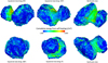 |
Fig. 1 Cumulative energy (in J m–2) from self-heating over one complete revolution of 67P. The range is truncated for a better visualisation; the values actually range from 0 to 8.2 × 10⁹ J m–2. The results were obtained with Model 1, which has 300 000 facets. |
2.1.2 Importance of self-heating
Adding self-heating to the model takes more computing time, but it is an important effect to take into account for 67P to properly calculate the surface temperature. To illustrate this point, we ran our thermal model with and without self-heating for comparison. As shown in Fig. 1, self-heating primarily affects the entire neck region where the two lobes of 67P face each other. It also affects the cliffs in general, all over the nucleus, because they see all the facets of the plain they dominate, and more particularly the cliffs in the neck, because they combine the two characteristics mentioned above (being a cliff and being in the neck). The cumulative self-heating energy varies from 0 to 8.2 × 10⁹ J m–2. For 5% of the facets, the energy from self-heating exceeds the energy received from the Sun over one revolution; most of these facets are located on cliffs in the neck.
We also calculated the changes in maximum temperature due to self-heating by comparing cases with and without self-heating. Figure 2 illustrates the results. The increase in the maximum temperature is >6 K for 50% of the facets, >18 K for 10% of the facets, and >33 K for 1% of the facets. The largest differences are found where self-heating is important (i.e. in the neck and on cliffs). Overall, this demonstrates the importance of including self-heating for an accurate surface temperature determination at 67P.
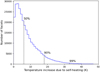 |
Fig. 2 Histogram of the temperature rise due to self-heating. The temperature increase is >6 K for 50% of the facets. |
2.2 Interior thermal model with conductivity (Model 2)
Here we present our second thermal model. Unlike the first model, this one takes into account the heat conductivity. Selfheating is neglected because we are interested in the temperature inside the nucleus, which is mainly driven by the thermal conductivity, and not by self-heating, which mainly affects the surface and plays a minor role in the subsurface. Furthermore, since we are interested in the maximum internal temperature, water ice sublimation is neglected and there is no gas flow (i.e. pure dust model). This model is also applied to the nucleus shape model SHAP7 of Preusker et al. (2017), but decimated to 10 000 facets. Our thermal model computes the temperature on the surface and inside the nucleus of 67P, down to ~3 m and for each facet of the shape model, at any time around its orbit. As for the first model, the geometric information is computed using the OASIS software (Jorda et al. 2010). The model takes into account projected shadows. Lateral heat conductivity is neglected. As for Model 1, if a facet is not illuminated, the insolation is artificially set to 0.
The upper boundary condition is the surface energy balance of a facet i of the shape model, given by Eq. (4):
 (4)
(4)
where κ is the heat conductivity and z is the depth. Inside the nucleus, the heat conductivity is solved using Eq. (5):
 (5)
(5)
where ρ is the density, and c is the specific heat capacity. For the lower boundary condition, we assumed a zero temperature gradient:
 (6)
(6)
We solved the above system of three equations by introducing the thermal inertia  . We used a standard value of Γ=50 J m–2 K–1 s–1/2 for the thermal inertia of cometary nuclei (see the review by Groussin et al. 2019), in agreement with the range 10–60 J m–2 K–1 s–1/2 derived from MIRO observations at 67P (Schloerb et al. 2015; Choukroun et al. 2015). The numerical resolution requires a time and depth step small enough to achieve numerical convergence, but large enough to limit computational time. After several tests, we find a good compromise with a time step of 24.8 s (i.e. 1800 time steps per rotation, which is more than 8 million time steps per revolution) and a depth step of one-tenth the diurnal thermal skin depth, ξ:
 (7)
(7)
where P is the period of rotation (or period of revolution for seasonal skin depth). Assuming a thermal inertia of 50 J m–2 K–1 s–1/2, a density of 532 kg m–3 (Jorda et al. 2016), and a specific heat capacity of 1000 J K–1 kg–1 (typical value for silicates; Drury et al. 1984), the diurnal skin depth equals 11.2 mm (i.e. a depth step of 1.12 mm). We calculated the temperature over 3000 depth steps (i.e. down to 3.4 m). This is more than four times the seasonal thermal skin depth of ~75 cm. With the above time step and depth step, the numerical model converges in less than 5 revolutions. In total, it takes about 10 days of computing time on a PC with 24 CPUs in parallel.
Ultimately, this thermal model provides the maximum surface temperature and temperature profiles down to a depth of ~3 m, at any time on 67P’s orbit, and for the 10 000 facets of the shape model.
3 Thermal environment
Here we explore the thermal environment of 67P on its current orbit using the two thermal models introduced in the previous section. We focus on the energy received from the Sun, the surface temperature, the temperature variations with time and depth, and the location of H2O and CO2 ices with depth. We refer to the SH for latitudes in the range [–90°; –30º], to the equator for latitudes in the range [–30°; +30°], and to the NH for latitudes in the range [+30°; +90°]. All 3D models used to generate the figures in this paper are made available to the scientific community in Appendix B.
3.1 Energy received from the Sun and from self-heating
Figure 3 shows the cumulative energy received from the Sun at the surface of 67P over one orbit. The energy varies from 0.1 × 10⁹ J m–2 to 8.5×10⁹ J m–2. The maximum insolation is at the equator, which is constantly illuminated all around the orbit. Insolation in the SH and NH is comparable, but on average 10% less than the maximum at the equator. The neck receives only 50% of the maximum insolation due to projected shadows. Cliffs, wherever they are (i.e. NH or SH), also receive about 50% of the maximum insolation, due to the fact that, unlike flatter areas, they are never illuminated all day. The regions with the lowest insolation are the cliffs located in the northern part of the neck, which receive only 20% of the maximum insolation. The anti-correlation between slope and insolation, with high- slope terrains (i.e. cliffs) receiving less energy from the Sun than low-slope terrains (i.e. plains), is statistically confirmed with a Pearson correlation coefficient of –0.63, indicating a strong anti-correlation.
Figure 4 shows the cumulative energy received from the Sun and from self-heating on the surface of 67P over one orbit, which we call the total energy. Unlike the insolation, the total energy is almost constant over the surface and equals to 7.5±0.1× 10⁹ J m–2 (i.e. variations of <15%). This results from the almost perfect anti-correlation between solar energy (Fig. 3) and self-heating energy (Fig. 1), with a Pearson correlation coefficient of –0.97. On the neck in general, and even more so on the cliffs neck where insolation is the lowest, self-heating is the strongest, so they compensate each other out. If we look more closely at the narrow range of total energy input, we see that the equator and cliffs have the highest energy input, while the neck area has the lowest. Over one orbit, with Model 1, the total energy from selfheating is 17% of the total energy budget, while the energy from the Sun is 83% of the total energy budget.
We also computed the duration of polar night over an orbit (Fig. A.1). Three regimes are clearly visible, resulting from seasonal effects due to the 52° obliquity of 67P. At the equator, which is constantly illuminated throughout the orbit, there is no polar night (0 days). In the NH, which is always illuminated except at perihelion, polar night is short (3–6 months). In the SH, which is illuminated only at perihelion, there is a long polar night that lasts for most of the orbit (~5 years). These seasonal effects play a fundamental role in understanding the thermal environment of 67P. In particular, there is a clear dichotomy between the SH and the NH: the SH experiences a strong insolation peak at perihelion and none for the rest of the orbit, while the NH experiences less insolation but for a much longer time than the SH.
3.2 Effects of heat conductivity
To quantify the effect of heat conduction, we ran Model 2 without heat conduction to evaluate the changes in maximum and minimum surface temperature over one revolution. As expected, thermal conduction decreases the maximum surface temperature by pumping energy from the surface on the day side, and increases the minimum surface temperature by returning energy from the nucleus interior to the surface on the night side. Quantitatively, thermal conduction decreases the maximum surface temperature by less than 10 K for 80% of the facets, and by more than 20 K for 5% of the facets; the largest differences are found in the NH, especially in the neck. For the minimum surface temperature, the changes are more important, and thermal conduction increases the minimum surface temperature by an average of 68 K, with values in the range 36–110 K; the largest differences are found at the equator. These larger changes result from the fact that the minimum temperature is always 0 K without thermal conduction. Over one orbit, with Model 2, the total energy from thermal conduction (either injected into or returned from the interior) is 34% of the total energy budget.
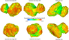 |
Fig. 3 Cumulative energy (in J m–2) received from the Sun at the surface of 67P over one orbit (same range as in Fig. 4 for ease of comparison). The results were obtained with Model 1. |
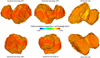 |
Fig. 4 Cumulative energy (in J m–2) received from the Sun and from self-heating at the surface of 67P over one orbit (same range as in Fig. 3 for ease of comparison). The results were obtained with Model 1. |
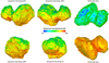 |
Fig. 5 Maximum temperature (in K) reached on the surface of 67P during one revolution. The range is truncated for better visualisation; the values actually range from 210 to 409 K. The results were obtained with Model 1. |
3.3 Surface temperature
Temperature is directly related to solar radiation, and varies daily and seasonally. We first examined the maximum temperature reached over the orbit, with Model 1 for pure dust (f = 0), illustrated by Fig. 5. Globally, the maximum temperature is highest in the SH (350–400 K), followed by the equatorial regions (300– 350 K), and then the NH, which is the coldest (210–300 K). This directly reflects the seasonal effects explained above. The coldest areas in the NH are located at the tops of each lobe (blue regions in Fig. 5), which remarkably correspond to the only areas on the nucleus where Barrington et al. (2023) observed a net zero balance between erosion and deposition over the orbit. The cliffs in the NH (e.g. in the Seth region) are significantly hotter than the surrounding plains, by 50–100 K; they are more prone to self-heating and their orientation allows for longer insolation when approaching the Sun, delaying the onset of polar night. At the equator (e.g. in the Imhotep region), cliffs facing south are 50 K hotter than the plains, while cliffs facing north are 50 K colder than the plains. Overall, cliffs and plains behave differently due to their different orientation relative to the Sun. Finally, the maximum temperature is always higher than the sublimation temperature of water ice (200 K), so there is no region on 67P’s surface where water ice is stable all around the orbit.
Figure 6 shows the minimum noon temperature over an orbit, which means that the temperature during the day always exceeds this value, no matter what day it is on the orbit. In other words, there is always a time during the orbit when it is warmer. In the SH and NH, the minimum noon temperature is 0 K, since it is the temperature reached during polar night with Model 1, which has no thermal inertia. Therefore, in the SH and NH, there is always a period along the orbit where water ice cannot sublimate (<150 K) and is stable on the surface. This conclusion does not change if the thermal inertia is not zero, for example with Γ=50 J m–2 K–1 s–1/2 for Model 2, since the night side temperature is always below 150 K all around the orbit for Model 2. At the equator, which by definition is illuminated every day of the orbit, the noon temperature is always positive, in the range 100– 190 K; water ice can be stable on the surface in some equatorial regions (<150 K), but not everywhere and mainly in north-facing cliffs.
Figure 7 shows the maximum rate of temperature change per minute (K min–1), over one revolution. The value varies from 3.0 to 17.3 K min–1, with a mean value of 9.7±2.1 K min–1. The lowest values of 3–5 K min–1 are found in the neck, more precisely in the NH. There is a moderate correlation between slope and rate of temperature change per minute (Pearson correlation coefficient >0.3), and the largest values >15 K min–1 are observed on the cliffs. This implies greater thermal fatigue for the outermost part of cliff faces compared to the rest of the nucleus.
3.4 Temperature at different depths
With Model 2 (10 000 facets) we can calculate the temperature inside the nucleus at different depths. Figure 8 shows the maximum temperature reached during one revolution at different depths: at the surface, at 5 cm depth (below the diurnal thermal skin depth) and at 1 m depth (below the seasonal thermal skin depth). The maximum surface temperature is slightly lower compared to Fig. 5 because self-heating is not included in Model 2, but conduction is. At 5 cm depth the temperature drops significantly, to 250–300 K in the SH and to 150–200 K in the NH. Sublimation of water ice is still possible everywhere, except on the cliffs on either side of the neck in the NH and in large deep holes in the NH. At 1 m depth the temperature is even lower, from 70 to 100 Kin the SH to 100–170 Kin the NH. Sublimation of water is only possible in the northern terrains that face north, such as in the Ma’at and Ash regions. Finally, sublimation of CO2 ice is possible everywhere in the nucleus down to 1 m depth, since the temperature is always >70 K.
In summary, the maximum temperature inside the nucleus at 1 m depth is lower in the SH than in the NH, because the SH receives a short and strong peak of solar radiation at perihelion, which heats the nucleus only superficially compared to the NH, which is heated for a much longer time, allowing the energy to penetrate deeper into the nucleus.
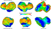 |
Fig. 6 Minimum noon temperature (in K) reached on the surface of 67P during one orbit. The results were obtained with Model 1. |
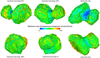 |
Fig. 7 Maximum rate of temperature change per minute (in K/min) at the surface of 67P over one revolution. The range is truncated for better visualisation; the values actually range from 3.0 to 17.3 K/min. The results were obtained using Model 1. |
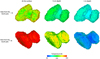 |
Fig. 8 Maximum temperature at different depths: at the surface, at 5 cm depth (below the diurnal thermal skin depth), and at 1 m depth (below the seasonal thermal skin depth). The results were obtained with Model 2, which has 10 000 facets. |
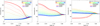 |
Fig. 9 Temperature as a function of time and depth for different plains (low slope terrains) located in the SH (left), at the equator (middle), and in the NH (right). The colour indicates time (heliocentric distance), with solid lines representing pre-perihelion and dashed lines representing post-perihelion. |
3.5 Temperature variation with time and depth
3.5.1 Plains (low slope terrain)
Model 2 allows us to plot temperature profiles for each facet as a function of time and depth. Figure 9 illustrates this point for several facets located in plains, in the SH, at the equator, and in the NH.
In the SH, the temperature regularly increases as the nucleus approaches perihelion (up to 350 K) and then decreases, with the minimum temperature at aphelion during polar night. During polar night, the temperature at the surface (50 K) is lower than inside the nucleus (100 K); this temperature inversion leads to possible condensation of CO2 in the first metre. The temperature inversion with depth results directly from the seasonal thermal wave structure. In the case of water, sublimation below 100 K is negligible and therefore water remains in the solid phase (ice) during polar night.
At the equator, we observe the same trend with an increase in temperature before perihelion (up to 330 K) and a decrease afterwards, but the surface temperature drops less at aphelion than in the SH because there is no polar night at the equator (125 K at the equator versus 50 K in the SH). The lack of polar night prevents the temperature inversion, and CO2 ice and water ice cannot condensate.
In the NH the trend is different. The temperature increases regularly as the nucleus approaches perihelion, but only up to 240 K (instead of 350 K in the SH), and then there is a sudden drop near perihelion as the NH enters polar night, from 240 to 70 K in a few days. This abrupt cooling leads to a strong temperature inversion, with an interior temperature above 150 K and a surface temperature close to 70 K. Under these conditions, CO2 ice and water ice can sublimate inside the nucleus and re-condensate in the first decimetres near the surface. The temperature at 3 m depth is also higher than in the SH (145 K in the NH versus 100 K in the SH), as shown earlier with Fig. 8.
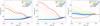 |
Fig. 10 Temperature as a function of time and depth for different cliffs (high slope terrains) located in the SH (left), at the equator facing south (middle), and in the NH (right). The colour indicates time (heliocentric distance), with solid lines representing pre-perihelion and dashed lines representing post-perihelion. |
3.5.2 Cliffs (high slope terrain)
Figure 10 is the same as Fig. 9 but for cliffs instead of plains. In the SH, the trend for cliffs is about the same as for plains, but cliffs are globally colder than plains. The temperature reached near perihelion is lower, 300 K for cliffs instead of 350 K for plains, and the heating is more superficial. At a depth of 10 cm, the temperature never exceeds 180 K for cliffs, while it reaches 250 K for plains. As for the plains, there is a temperature inversion during polar night, where CO2 can sublimate in the nucleus and re-condensate at shallower depths. However, the temperature is too cold for the sublimation of water ice to take place during polar night, and water remains in the solid phase. At the equator, the south-facing cliffs behave exactly like the plains in the SH, with a regular pre-perihelion temperature rise (up to 350 K), a post-perihelion temperature decrease (down to 50 K at aphelion), and a long temperature inversion curve during polar night, during which CO2 can sublimate inside and re-condensate at shallower depths. In the NH, cliffs follow the same trend as plains, with the notable difference that the maximum temperature reached before entering polar night near perihelion is higher (300 K) than for plains (240 K). On the contrary, the internal temperature is slightly lower for cliffs (130 K) than for plains (145 K).
3.6 Location of the H2O and CO2 ices as a function of depth
From the temperature profiles computed on each facet with Model 2, we can look for the maximum temperature reached at different depths, and in particular we can look for the isotherm 150 K, which is a threshold where the sublimation of water ice becomes negligible (∼1 mm of erosion per revolution). Figure 11 illustrates this point and shows the depth at which the temperature never exceeds 150 K. We note that our model overestimates this depth, which should be considered as an upper limit, since Model 2 considers only dust (no ices), whereas the presence of ices inside the nucleus would lower the temperature, since sublimation is an endothermic process.
Even with the above limitations, it is striking that in the northern part of the neck and the surrounding cliffs, water ice is always very close to the surface, within the first few millimetres. As we will see in Figs. 14 and 15, this is due to the very cold environment at this location, which only allows sublimation of water ice during a short period (a few months) around perihelion.
From the temperature profiles, we also looked for temperature inversion, where the interior of the nucleus is hotter than the surface, allowing ice to sublimate in the interior and condensate near the surface. More specifically, we looked for places where the temperature increases monotonically with depth, starting from <150 K at the surface for water (i.e. stable water ice) and <70 K for CO2 (i.e. stable CO2 ice). Examples of such temperature inversion curves can be seen in the right panel of Fig. 9 for water near perihelion (thick red curve) and in the left panel of Fig. 9 for CO2 near aphelion (thick blue curve). Figure 12 shows for each facet the time during which condensation of water or CO2 is possible. These are seasonal condensation effects, which would allow a significant amount of ice to accumulate near the surface, rather than diurnal effects, which would allow ice to condensate locally as frost.
For water, condensation is not possible in the SH because the internal temperature is always too low to allow the sublimation of water ice and therefore its condensation at shallower depths. In the NH, condensation of water ice is possible, but only outside the neck and for facets facing north. The condensation time is 10–20% of the revolution period and occurs during the short (a few months) polar night near perihelion.
For CO2, condensation is possible in the NH and in the SH, but not at the equator. In the SH, CO2 can condensate during up to 80% of the revolution period during the long (about 5 years) polar night at aphelion. In the NH, condensation is also possible during 10–40% of the revolution period. At the equator, where by definition there is no polar night, the surface temperature remains constantly above the sublimation point of CO2 ice and condensation is therefore not possible. The CO2 condensation time correlates very well with the duration of polar night (compare Fig. A.1 with Fig. 12).
In summary, it is possible for water ice to accumulate in the subsurface layers near perihelion in the NH, and for CO2 ice to accumulate in the NH and SH, with the possibility of large CO2 accumulations at aphelion in the SH.
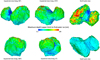 |
Fig. 11 Depth (upper limit) at which the sublimation of water ice becomes negligible (~1 mm of erosion per revolution), which happens when the maximum temperature never exceeds 150 K. The results were obtained with Model 2. |
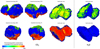 |
Fig. 12 Timescale over which CO2 and H20 can condensate when there is an inversion of the temperature gradient (colder near the surface than inside). The results were obtained with Model 2. We use a logarithmic scale. |
4 Erosion
We calculated the erosion with Model 1, assuming pure water ice (i.e. with a value of f=1 in Eq. (1)). The resulting erosion is overestimated because the nucleus is not pure water ice, so we scaled the erosion so that the total production rate from our model over one revolution matches the total mass loss measured during the Rosetta mission. The total mass loss was first estimated to be 10.5 × 10⁹ kg by Pätzold et al. (2019) from the RSI (Radio Science Investigation) radio science experiment on board Rosetta. More recently, by adding constraints from OSIRIS (Optical, Spectrocopic and Infrared Remote Imaging System) images to the RSI data, Laurent-Varin et al. (2024) revised this mass loss to 28.0×10⁹ kg; we used this later value here. The resulting erosion is shown in Fig. 13. As our model does not take dust transport and associated dust deposition into account, this is a theoretical erosion that does not represent the actual locally measured erosion.
The expected erosion varies across the surface, from ~25 cm in the NH to ~190 cm in the SH. The least eroded terrains (25– 50 cm) are the north-facing plains and the neck in the NH, while the most eroded terrains (150–190 cm) are the plains and the neck in the SH, as well as the south-facing cliffs at the equator. The intermediate eroded terrains (50–150 cm) are the cliffs in the NH, the plains at the equator, and the north-facing cliffs at the equator. As already seen for the maximum temperature, cliffs and plains behave differently due to their different orientation. In general, the maximum temperature correlates very well with erosion, with a Pearson correlation coefficient of 0.94. This correlation is expected because erosion is proportional to the production rate, which is an exponential of temperature (Eq. (2)), so the hottest regions are also the most eroded.
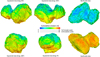 |
Fig. 13 Erosion (in m) at the surface of 67P over one revolution, calculated with Model 1 assuming pure water ice (f =1 in Eq. (1)). Two scales are shown for the colour bar: one corresponding to our model with pure water ice (model scale) and one corresponding to the same model but scaled to the total mass loss derived from RSI data and OSIRIS images (realistic scale). The results were obtained with Model 1. |
5 Some examples of applications
The results of our two thermal models presented above can be used to address many scientific questions related to 67P and comets in general. Here are three examples of applications to illustrate this point, within the limitations of our models: two related to surface morphological changes (Sects. 5.1 and 5.2), and one related to the seasonal variations in H2 O and CO2 (Sect. 5.3).
5.1 Cliff collapse in the Aswan region
In July 2015, a cliff collapse occurred in the Aswan region of 67P, causing an outburst. This event has been studied in detail by Pajola et al. (2017) and Davidsson (2024a). The Aswan region is located in the NH and more precisely in the neck (Fig. 14, top left). The collapse occurred a few weeks before perihelion. According to Pajola et al. (2017), itis caused by the gradual opening of fractures due to diurnal and seasonal thermal gradients (i.e. thermal stress), which weakened the cliff and enhanced the sublimation of ice.
With our work, we have additional arguments to explain this cliff collapse, illustrated by Fig. 14. First, the cliff collapse occurred in a very peculiar and localised area of the cliff, where polar night is locally much longer than in the surrounding area (lower-left panel). This peculiar thermal environment is due to the overhanging position of this cliff. This long polar night induces a long period of temperature inversion, allowing CO2 to accumulate in the subsurface (upper-right panel). At the same time, the water remains close to the surface (<6 cm) because there was only a short period of heating at perihelion, short enough that the water front does not recede to greater depths (lower right panel). Finally, the collapse occurred in July 2015, exactly when the temperature profiles with depth reached their maximum (upper-right panel).
The above arguments support the presence of near-surface volatiles, as suggested by Pajola et al. (2017), and are consistent with the work of Davidsson (2024a), who inferred a thin dust mantle (>3 cm) in the Aswan cliff before the collapse from MIRO observations. The presence of CO2 is particularly interesting since it is a super-volatile whose sublimation near perihelion may have weakened the sub-surface materials, facilitating their collapse due to the overhanging situation. Our study also explains why the cliff collapse occurred at this particular location, which has a peculiar thermal environment compared to the neighbouring cliffs, and why it occurred just before perihelion, when the subsurface temperature was at its maximum.
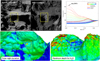 |
Fig. 14 Thermal environment of the cliff collapse observed in the Aswan region. Upper-left panel: two OSIRIS/NAC images of the Aswan cliff before and after the collapse, adapted from Pajola et al. (2017). Upper-right panel: temperature as a function of time and depth at the site of the cliff collapse, similar to Fig. 9. Lower-left panel: duration of polar night, extracted from Fig. A.1. Lower-right panel: maximum depth for water, extracted from Fig. 11. In all panels, the yellow box indicates the location of the cliff collapse. |
5.2 Surface changes in Hapi
Surface morphological changes have been observed in the Hapi region, studied in detail by Davidsson et al. (2022). The Hapi region is located in the neck, in the NH. These morphological changes take the form of growing depressions, about 140 m wide and 0.5 m deep, and result from the sublimation of CO2 near the surface, which according to the authors ejects dust and water ice outwards. The various thermophysical models used by Davidsson et al. (2022) to draw the above conclusions are constrained by MIRO observations, and the models are run from the time of aphelion to the time of the MIRO observations and beyond (i.e. from May 2012 to March 2015; the MIRO observations were performed October–November 2014). In our work, we used a less detailed thermophysical model, but it is run over a full orbit, which adds further arguments to support the above conclusions.
In Fig. 15 we show the temperature as a function of time and depth at the location of the surface morphological changes observed in the Hapi region. The temperature was calculated with Model 2, which assumes pure dust (no ice). The first result is that the temperature at this location never exceeds 220 K, so it is a very cold environment (see also Fig. 5). As shown in Fig. A.1, this region is in permanent night for 7 months around perihelion, avoiding extreme high temperatures. It is also striking that the time of the observed changes (December 2014–March 2015) coincides exactly with the maximum temperature, just before entering polar night. Finally, the condensation of CO2 and its accumulation in the first metres is possible during the 7 months of permanent night at perihelion, enriching the subsurface in CO2 in this region. However, to explain the observed changes, CO2 must remain close to the surface after perihelion until aphelion, which could only be possible if it is thermally isolated from the outside by an insulating layer: either a layer of dust deposited on the surface around perihelion (Barrington et al. 2023) or a layer of water ice that pumps all the energy coming from the Sun by sublimation (Hoang et al. 2019). Overall, the above conclusions strengthen the scenario of Davidsson et al. (2022) where CO2 is the driver of the observed surface morphological changes in Hapi, and in particular support a high enrichment in CO2 (~30% relative to water) within the first decimetres required to initiate the changes.
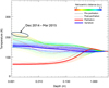 |
Fig. 15 Temperature as a function of time and depth at the location of the surface morphological changes observed in the Hapi region. The colour indicates the time (heliocentric distance), with solid lines representing pre-perihelion and dashed lines representing post-perihelion. |
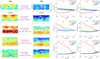 |
Fig. 16 Column density maps for H2O (first column) and CO2 (second column) at different heliocentric distances, from ROSINA/RTOF observations; the figure is adapted from Hoang et al. (2019). The temperature profiles with time and depth corresponding to locations A to F on the maps, computed with Model 2, are shown in the third and fourth columns. |
5.3 Seasonal variations in H2O and CO2
The seasonal variations in H2O and CO2 have been studied by several authors, in particular Fougere et al. (2016), Läuter et al. (2019), Hoang et al. (2019, 2020), and Davidsson et al. (2022), all based on ROSINA mass spectrometer observations.
Fougere et al. (2016) suggested that: (i) the NH is depleted in CO2 but not in H2O, and hence H2O dominates at large heliocentric distances, and (ii) the SH undergoes rapid erosion around perihelion, constantly exposing new materials (H2O and CO2) at the surface (i.e. following the erosion front). Hoang et al. (2019) produced production maps of H2O and CO2 at different heliocentric distances and concluded that: (i) H2O production correlates with insolation, (ii) there is more CO2 in the SH because it is more eroded and pristine, (ii) and that a vertical stratification with three layers (dust + H2O / pure H2O / CO2 + CO) can explain the observations where far from the Sun CO2 and CO sublimate (too cold for H2O), while close to the Sun, H2O sublimates and consumes all the energy, so that CO2 and CO production decrease because they are below H2O. Läuter et al. (2022) show that in the SH the seasonal CO2 outgassing follows the solar irradiation, whereas in the NH the outgassing does not coincide with the maximum irradiation conditions. H2O is more strongly linked to the seasonal illumination, but requires a minimum irradiation of about 50 W/m−2 to get activated. Davidsson et al. (2022) interpreted the ROSINA data presented in Fougere et al. (2016) with their thermophysical model (NIMBUS) and came to the following conclusions: (i) H2O is always located below a thin dust mantle of 1–2 cm (except at latitude 5 N where the dust mantle is 15 cm thick), (ii) CO2 is located 1.9 m deep in NH and 3.9 m deep in SH near the aphelion, and a few decimetres below the surface around perihelion, following the erosion front, and (iii) there is more CO2 in the SH (32% relative to H2O) than in the NH (11% relative to H2O).
In summary, the above previous works agree on a SH enriched in CO2 compared to the NH, and H2O and CO2 close to the surface around perihelion in the SH, following the erosion front. However, they disagree on which volatile dominates around aphelion, H2O according to Fougere et al. (2016), CO2 according to Hoang et al. (2019).
Our global study of the thermal environment of 67P provides additional arguments to explain the observed seasonal variations. Figure 16 shows the density maps of H2O and CO2 at different heliocentric distances from Hoang et al. (2019), together with temperature profiles as a function of time and depth for different locations (latitude +60°N, 0° and −60°S) derived from Model 2. Locations A, C, E are inside the neck, while B, D, F are outside the neck. We focus here on some observational constraints that can be explained by our models.
5.3.1 The seasonal variations in H2O
For H2O, as suggested by Hoang et al. (2019), the general trend follows the insolation, with more H2O at smaller heliocentric distances. If we look at the temperature profiles, we can see that all regions in red on the H2O maps correspond to a place and time where the surface temperature exceeds 200 K (i.e. a strong sublimation rate of H2O). This sensitivity of H2O to surface temperature is a good indication that water ice is never far from the surface, within the first few centimetres according to Davidsson et al. (2022).
Beyond this general trend for H2O, one can see some subtleties for sites A and B, which experience a short polar night at perihelion as shown in the temperature profiles. At these two high latitude sites, the production rate is expected to decrease around perihelion and remain low after perihelion. While we unfortunately do not have a density map at perihelion, the postperihelion map (1.8–2.4 au) does indeed confirm the above prediction, as it shows a transition region around latitude +60°N where H2O is much lower compared to the equator and SH. Continuing with locations A and B, the two pre-perihelion H2O maps show that more H2O is produced outside the neck (location B) than inside the neck (location A). Since the temperature profile at location B is systematically larger by 10–20 K compared to location A, this provides a natural explanation to understand this observation.
5.3.2 The seasonal variations in CO2
CO2 does not show the longitudinal variations that we see for H2O, for example between sites A and B. The flux depends only on latitude and time, not on longitude. This shows that CO2 is less sensitive to surface temperature and more affected by seasonal temperature variations (i.e. at greater depths than H2O). From our temperature profiles we see that at a depth of 75 cm, which corresponds to the seasonal thermal skin depth, the seasonal temperature variations are <30 K in the NH, <40 K at the equator, and <60 K in the SH. For seasonal temperature variations below 10 K (i.e. an almost constant CO2 flux), one has to go deeper, about 2 m below the surface.
In the NH the CO2 flux is always low, except after perihelion. It is likely that CO2 is buried deep enough to produce an almost constant diffuse background of CO2 (i.e. about 2 m below the surface), as mentioned above. During polar night at perihelion (see the temperature profiles for locations A and B), CO2 accumulates near the surface in the first decimetre, which explains the higher flux observed after this polar night, post-perihelion, when the interior temperature rises again. The amount of CO2 accumulated near the surface during polar night is sufficient to produce a stronger flux for a few weeks, but not longer; this new reservoir formed near the surface empties rapidly.
In the SH, the CO2 flux increases regularly as the comet approaches the Sun, indicating a shallower location than in the NH, probably within the first metre according to the temperature profiles for locations E and F. The CO2 flux remains stable post-perihelion for a long time, at least up to 3 a.u. It is only when the surface cools to below 70 K, at about 4 a.u. according to the temperature profiles E and F, that the CO2 flux is expected to decrease rapidly. CO2 will then accumulate during the long polar night, in the first decimetre, and will then be released when approaching the Sun at the next perihelion passage, when leaving polar night. It is worth mentioning that pre-perihelion, at a distance of 3.1–2.3 a.u., the SH is still in polar night (temperature profiles E and F), so one would expect a very low CO2 flux. However, while this is true for plains, it is not the case for cliffs, as shown in Fig. 10 (left panel). In fact, cliffs in the SH start to be illuminated before plains, with an earlier temperature rise. The observed CO2 flux at this time therefore comes from the southern cliffs, not from the plains.
The equator is a transition region from NH to SH and shows a gradual increase in CO2 flux with decreasing heliocentric distance. This transition can be understood because the equator is a mixture of plains, north-facing cliffs and south-facing cliffs, and therefore contains different thermal environments. In the plains, CO2 is expected to be deeply buried due to the lack of polar night, as it never accumulates near the surface in the first few metres. One would therefore expect a more constant and lower flux of CO2 compared to the NH or SH. Unfortunately, due to the low spatial resolution of the CO2 flux map, we cannot distinguish plains from cliffs at the equator, and we cannot confirm this lower CO2 flux for plains.
Overall, the CO2 flux seems to be driven by the seasonal variations in temperature with depth, and in particular by the duration of polar night. Because polar night is 10 times longer in the SH compared to the NH, there is more time for CO2 to accumulate near the surface in the SH, and the near surface region of the SH is therefore enriched in CO2 compared to the NH.
6 Conclusions
We have studied in detail the thermal environment and erosion of comet 67P over a complete revolution. Over one orbit, the total energy from self-heating is 17% of the total energy budget (estimated from Model 1), while the total energy from thermal conduction (either injected into or returned from the interior) is 34% of the total energy budget (estimated from Model 2). Table 1 summarises our results. Due to the high obliquity of 67P (52°), seasonal effects greatly impact the thermal environment but in different ways for the NH, the equator, and the SH.
6.1 Northern hemisphere (latitude [+30° ;+90°])
The NH is always illuminated, except for a short polar night that lasts 3 to 6 months around perihelion. The NH misses the strongest insolation at perihelion and is therefore the coldest region of the nucleus, with a maximum surface temperature in the range 210–300 K. The neck, which is subject to shading effects, and the cliffs, which are exposed to sunlight for only part of the day, both receive only 50% of the maximum amount of solar energy. However, this is offset by a significant increase in temperature due to self-heating in the neck and cliffs, which raises the surface temperature by 20 K or more.
When the NH enters polar night, the surface cools very rapidly (down to 70 K in a few days) and a temperature inversion with depth occurs; the surface becomes colder than the interior. This temperature inversion means that the sublimation of H2O and CO2 ices continues inside the nucleus and they condensate at shallower depths, close to the surface, where they cannot sublimate (temperatures below 70 K). They therefore accumulate in the first few centimetres. Combined with the ROSINA/RTOF observations, our results suggest that H2O is always within the first few centimetres, while CO2 is deeper, about 2 m below the surface, except during polar night when CO2 can accumulate close to the surface. The amount of CO2 accumulated near the surface during polar night is sufficient to produce a stronger flux of CO2 for a few weeks when polar night comes to an end, but not longer; this new reservoir formed near the surface empties rapidly.
Finally, due to their different orientations, cliffs erode 3 to 5 times faster than plains and experience stronger thermal gradients, of up to 15 K min−1. This translates to more thermal fatigue of the outermost portion (i.e. centimetres) of the cliffs. Thus, in the NH, erosion preferentially occurs on cliffs (high slope terrains), which explains the observed terraces.
Thermal environment synthesis for various locations and parameters.
6.2 Equator (latitude [−30° ;+30°])
Unlike the NH, the equator is, by definition, always illuminated and without polar night. It is here that the cumulative energy received from the Sun is at its maximum, with 8.5×10⁹ J m−2. The maximum surface temperature is also higher than in the NH, in the range 300–350 K.
Because of the lack of polar night, the noon temperature is always too high to allow the presence of H2O and CO2 ice on the surface for a full day, except on north-facing cliffs. On the plains, there is no temperature inversion with depth on the seasonal timescale, and CO2 is expected to be buried about 2 m below the surface, never able to accumulate near the surface in the upper decimetres. As in the NH, H2O ice is likely to reside within the first few centimetres, with its sublimation helping explain the observed regular increase in H2O flux with decreasing heliocentric distance.
The cliffs differ from the plains and can be divided into two categories: the north-facing cliffs, which have a thermal environment similar to that of the NH, and the south-facing cliffs, which have a thermal environment similar to that of the SH. As expected, erosion is greater on south-facing cliffs than on plains or north-facing cliffs.
Overall, the equatorial region, which is a mixture of plains and cliffs, is a transitional region between NH and SH.
6.3 Southern hemisphere (latitude [−90° ;−30°])
The SH is illuminated only around perihelion for 3–6 months and is in polar night for the rest of 67P’s orbit. It experiences the strongest and fastest thermal variations, going from polar night to maximum insolation and then back to polar night, all within a few months around perihelion. The maximum temperature is in the range 350–400 K around perihelion and drops to 55 K during polar night. There is a noticeable difference between plains and cliffs, as the maximum temperature on cliffs is about 50 K colder than on plains and the heating is more superficial (10 cm below the surface, the temperature never exceeds 180 K on cliffs but can reach 250 K on plains).
Due to the short insolation time, solar energy does not penetrate as deep into the subsurface as in the NH. At 1 m below the surface, the temperature in the SH is in the range 70–100 K, lower than the 100–170 K observed in the NH. Combined with the ROSINA/RTOF observations, our results suggest that H2O is always within the first few centimetres, as in the NH. Around perihelion, when the nucleus is illuminated, CO2 is located within the first metre. Out of perihelion, during polar night, CO2 can accumulate near the surface due to the temperature inversion (the surface becomes colder than the interior). Compared to the NH, the period of accumulation of CO2 near the surface is much longer, about 5 years. Larger amounts of CO2 ice are therefore expected to accumulate in the first decimetre compared to the NH. This helps explain why the SH appears to be richer in CO2 than the NH, as this large, near-surface reservoir of CO2 will begin to sublimate as the comet approaches the Sun, first from the cliffs at around 2.5–3.0 a.u. and then from the plains around perihelion. After perihelion, the CO2 flux will not decrease significantly until the surface cools to below 70 K.
Finally, erosion is maximum in the SH, about 7 times more than in the NH and 2 times more than at the equator. Compared to the NH, erosion preferentially occurs on plains (low slope terrains) rather than on cliffs (high slope terrains), which explains the observed overall flatness of this hemisphere, at large scales, compared to the NH.
6.4 Understanding nucleus surface changes
Our detailed study of the thermal environment also helps us better understand the observed changes on 67P’s surface, as illustrated by two examples: the cliff collapse in the Aswan region and the morphological changes within the smooth terrains of Hapi. For the cliff collapse, our study shows that it occurred in a peculiar region of the neck, which, due to the overhanging situation of this cliff, experiences a much longer polar night than its local neighbourhood; there is an enrichment of CO2 in the first decimetre during this long polar night; this may have helped trigger the collapse, which occurred exactly when the subsurface temperature was at its maximum. For the surface changes observed in the Hapi region, our study further confirms the importance of near-surface CO2 , same as Davidsson et al. (2022), and shows that the observed changes also occurred at maximum temperature, just as for the cliff collapse. These are just two examples of surface changes known to occur on 67P, and they serve to illustrate how our methods can help us understand the fine-scale evolution of the comet’s surface. Extending this work to other surface changes (e.g. El-Maarry et al. 2017; Birch et al. 2019; Jindal et al. 2022; Barrington et al. 2023; Jindal et al. 2024) is a promising endeavour that will be left to follow-up studies.
Acknowledgements
The contribution of O.G. and L.J. to this project was funded by the Centre National d’Etudes Spatiales (CNES). This research was supported by the International Space Science Institute (ISSI) in Bern, through ISSI International Team project #547 (Understanding the Activity of Comets Through 67P’s Dynamics). N.A. and P.G. acknowledge financial support from project PID2021-126365NB-C21 (MCI/AEI/FEDER, UE) and from the Severo Ochoa grant CEX2021-001131-S funded by MCI/AEI/10.13039/501100011033. We thank the reviewer, O. M. Umurhan, for his helpful and constructive report.
Appendix A Additional figure
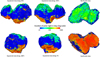 |
Fig. A.1 Duration of polar night over one complete orbit of 67P (in days). The range is truncated for better visualisation; the values actually range from 0 days to 2300 days. The results were obtained with Model 1. |
Appendix B Links to access the 3D colour VRML models
All 3D models used to generate the figures in this paper are available to the scientific community. The 3D models are provided in VRML (Virtual Reality Markup Language) format, using a rainbow colour table. The VRML format can be read by a variety of software, for example MeshLab, which is an open source software (https://www.meshlab.net). The list of 3D VRML models is provided in Table B.1, with the link to access the 3D models on the cloud from the Laboratoire d’Astrophysique de Marseille (France).
List of 3D models used to generate the figures in this paper.
References
- Attree, N., Jorda, L., Groussin, O., et al. 2019, A&A, 630, A18 [NASA ADS] [CrossRef] [EDP Sciences] [Google Scholar]
- Barrington, M. N., Birch, S. P. D., Jindal, A., et al. 2023, J. Geophys. Res. Planets, 128, e2022JE007723 [NASA ADS] [CrossRef] [Google Scholar]
- Birch, S. P. D., Hayes, A. G., Umurhan, O. M., et al. 2019, Geophys. Res. Lett., 46, 12794 [NASA ADS] [CrossRef] [Google Scholar]
- Bouquety, A., Groussin, O., Jorda, L., et al. 2022, A&A, 662, A72 [NASA ADS] [CrossRef] [EDP Sciences] [Google Scholar]
- Choukroun, M., Keihm, S., Schloerb, F. P., et al. 2015, A&A, 583, A28 [NASA ADS] [CrossRef] [EDP Sciences] [Google Scholar]
- Crifo, J. F. 1987, A&A, 187, 438 [NASA ADS] [Google Scholar]
- Davidsson, B. J. R. 2024a, MNRAS, 527, 112 [Google Scholar]
- Davidsson, B. J. R. 2024b, MNRAS, 529, 2258 [NASA ADS] [CrossRef] [Google Scholar]
- Davidsson, B. J. R., Sierks, H., Güttler, C., et al. 2016, A&A, 592, A63 [NASA ADS] [CrossRef] [EDP Sciences] [Google Scholar]
- Davidsson, B. J. R., Samarasinha, N. H., Farnocchia, D., & Gutiérrez, P. J. 2022, MNRAS, 509, 3065 [Google Scholar]
- Dones, L., Weissman, P. R., Levison, H. F., & Duncan, M. J. 2004, in Comets II, eds. M. C. Festou, H. U. Keller, & H. A. Weaver (Tucson: University Arizona Press), 153 [Google Scholar]
- Drury, M. J., Allen, V., & Jessop, A. M. 1984, Icarus, 103, 321 [Google Scholar]
- Duncan, M., Levison, H., & Dones, L. 2004, in Comets II, eds. M. C. Festou, H. U. Keller, & H. A. Weaver (Tucson: University Arizona Press), 193 [Google Scholar]
- El-Maarry, M. R., Groussin, O., Thomas, N., et al. 2017, Science, 355, 1392 [Google Scholar]
- Fanale, F. P., & Salvail, J. R. 1984, Icarus, 60, 476 [NASA ADS] [CrossRef] [Google Scholar]
- Fornasier, S., Hasselmann, P. H., Barucci, M. A., et al. 2015, A&A, 583, A30 [NASA ADS] [CrossRef] [EDP Sciences] [Google Scholar]
- Fougere, N., Altwegg, K., Berthelier, J. J., et al. 2016, MNRAS, 462, S156 [NASA ADS] [CrossRef] [Google Scholar]
- Groussin, O., Attree, N., Brouet, Y., et al. 2019, Space Sci. Rev., 215, 29 [Google Scholar]
- Hoang, M., Garnier, P., Gourlaouen, H., et al. 2019, A&A, 630, A33 [NASA ADS] [CrossRef] [EDP Sciences] [Google Scholar]
- Hoang, H. V., Fornasier, S., Quirico, E., et al. 2020, MNRAS, 498, 1221 [NASA ADS] [CrossRef] [Google Scholar]
- Hu, X., Shi, X., Sierks, H., et al. 2017a, MNRAS, 469, S295 [NASA ADS] [CrossRef] [Google Scholar]
- Hu, X., Shi, X., Sierks, H., et al. 2017b, A&A, 604, A114 [NASA ADS] [CrossRef] [EDP Sciences] [Google Scholar]
- Jindal, A. S., Birch, S. P. D., Hayes, A. G., et al. 2022, Planet. Sci. J., 3, 193 [NASA ADS] [CrossRef] [Google Scholar]
- Jindal, A. S., Birch, S. P. D., Hayes, A. G., et al. 2024, J. Geophys. Res. Planets, 129, e2023JE008089 [NASA ADS] [CrossRef] [Google Scholar]
- Jorda, L., Spjuth, S., Keller, H. U., Lamy, P., & Llebaria, A. 2010, Proc. SPIE, 7533, 753311 [NASA ADS] [CrossRef] [Google Scholar]
- Jorda, L., Gaskell, R., Capanna, C., et al. 2016, Icarus, 277, 257 [Google Scholar]
- Keller, H. U., Mottola, S., Davidsson, B., et al. 2015, A&A, 583, A34 [NASA ADS] [CrossRef] [EDP Sciences] [Google Scholar]
- Keller, H. U., Mottola, S., Hviid, S. F., et al. 2017, MNRAS, 469, S357 [Google Scholar]
- Lamy, P., Faury, G., Romeuf, D., & Groussin, O. 2024, MNRAS, submitted [arXiv:2401.02174] [Google Scholar]
- Laurent-Varin, J., James, T., Marty, J.-C., et al. 2024, Icarus, 424, 116284 [NASA ADS] [CrossRef] [Google Scholar]
- Läuter, M., Kramer, T., Rubin, M., & Altwegg, K. 2019, MNRAS, 483, 852 [Google Scholar]
- Läuter, M., Kramer, T., Rubin, M., & Altwegg, K. 2022, ACS Earth Space Chem., 1c00378 [Google Scholar]
- Marshall, D., Groussin, O., Vincent, J. B., et al. 2018, A&A, 616, A122 [NASA ADS] [CrossRef] [EDP Sciences] [Google Scholar]
- Pajola, M., Höfner, S., Vincent, J. B., et al. 2017, Nat. Astron., 1, 0092 EP [NASA ADS] [CrossRef] [Google Scholar]
- Pätzold, M., Andert, T. P., Hahn, M., et al. 2019, MNRAS, 483, 2337 [CrossRef] [Google Scholar]
- Preusker, F., Scholten, F., Matz, K. D., et al. 2017, A&A, 607, L1 [NASA ADS] [CrossRef] [EDP Sciences] [Google Scholar]
- Schloerb, F. P., Keihm, S., von Allmen, P., et al. 2015, A&A, 583, A29 [NASA ADS] [CrossRef] [EDP Sciences] [Google Scholar]
- Skorov, Y., Keller, H. U., Mottola, S., & Hartogh, P. 2020, MNRAS, 494, 3310 [NASA ADS] [CrossRef] [Google Scholar]
- Umurhan, O. M., Grundy, W. M., Bird, M. K., et al. 2022, Planet Sci. J., 3, 110 [CrossRef] [Google Scholar]
- Whipple, F. L. 1950, ApJ, 111, 375 [NASA ADS] [CrossRef] [Google Scholar]
All Tables
All Figures
|
Fig. 1 Cumulative energy (in J m–2) from self-heating over one complete revolution of 67P. The range is truncated for a better visualisation; the values actually range from 0 to 8.2 × 10⁹ J m–2. The results were obtained with Model 1, which has 300 000 facets. |
| In the text | |
|
Fig. 2 Histogram of the temperature rise due to self-heating. The temperature increase is >6 K for 50% of the facets. |
| In the text | |
|
Fig. 3 Cumulative energy (in J m–2) received from the Sun at the surface of 67P over one orbit (same range as in Fig. 4 for ease of comparison). The results were obtained with Model 1. |
| In the text | |
|
Fig. 4 Cumulative energy (in J m–2) received from the Sun and from self-heating at the surface of 67P over one orbit (same range as in Fig. 3 for ease of comparison). The results were obtained with Model 1. |
| In the text | |
|
Fig. 5 Maximum temperature (in K) reached on the surface of 67P during one revolution. The range is truncated for better visualisation; the values actually range from 210 to 409 K. The results were obtained with Model 1. |
| In the text | |
|
Fig. 6 Minimum noon temperature (in K) reached on the surface of 67P during one orbit. The results were obtained with Model 1. |
| In the text | |
|
Fig. 7 Maximum rate of temperature change per minute (in K/min) at the surface of 67P over one revolution. The range is truncated for better visualisation; the values actually range from 3.0 to 17.3 K/min. The results were obtained using Model 1. |
| In the text | |
|
Fig. 8 Maximum temperature at different depths: at the surface, at 5 cm depth (below the diurnal thermal skin depth), and at 1 m depth (below the seasonal thermal skin depth). The results were obtained with Model 2, which has 10 000 facets. |
| In the text | |
|
Fig. 9 Temperature as a function of time and depth for different plains (low slope terrains) located in the SH (left), at the equator (middle), and in the NH (right). The colour indicates time (heliocentric distance), with solid lines representing pre-perihelion and dashed lines representing post-perihelion. |
| In the text | |
|
Fig. 10 Temperature as a function of time and depth for different cliffs (high slope terrains) located in the SH (left), at the equator facing south (middle), and in the NH (right). The colour indicates time (heliocentric distance), with solid lines representing pre-perihelion and dashed lines representing post-perihelion. |
| In the text | |
|
Fig. 11 Depth (upper limit) at which the sublimation of water ice becomes negligible (~1 mm of erosion per revolution), which happens when the maximum temperature never exceeds 150 K. The results were obtained with Model 2. |
| In the text | |
|
Fig. 12 Timescale over which CO2 and H20 can condensate when there is an inversion of the temperature gradient (colder near the surface than inside). The results were obtained with Model 2. We use a logarithmic scale. |
| In the text | |
|
Fig. 13 Erosion (in m) at the surface of 67P over one revolution, calculated with Model 1 assuming pure water ice (f =1 in Eq. (1)). Two scales are shown for the colour bar: one corresponding to our model with pure water ice (model scale) and one corresponding to the same model but scaled to the total mass loss derived from RSI data and OSIRIS images (realistic scale). The results were obtained with Model 1. |
| In the text | |
|
Fig. 14 Thermal environment of the cliff collapse observed in the Aswan region. Upper-left panel: two OSIRIS/NAC images of the Aswan cliff before and after the collapse, adapted from Pajola et al. (2017). Upper-right panel: temperature as a function of time and depth at the site of the cliff collapse, similar to Fig. 9. Lower-left panel: duration of polar night, extracted from Fig. A.1. Lower-right panel: maximum depth for water, extracted from Fig. 11. In all panels, the yellow box indicates the location of the cliff collapse. |
| In the text | |
|
Fig. 15 Temperature as a function of time and depth at the location of the surface morphological changes observed in the Hapi region. The colour indicates the time (heliocentric distance), with solid lines representing pre-perihelion and dashed lines representing post-perihelion. |
| In the text | |
|
Fig. 16 Column density maps for H2O (first column) and CO2 (second column) at different heliocentric distances, from ROSINA/RTOF observations; the figure is adapted from Hoang et al. (2019). The temperature profiles with time and depth corresponding to locations A to F on the maps, computed with Model 2, are shown in the third and fourth columns. |
| In the text | |
|
Fig. A.1 Duration of polar night over one complete orbit of 67P (in days). The range is truncated for better visualisation; the values actually range from 0 days to 2300 days. The results were obtained with Model 1. |
| In the text | |
Current usage metrics show cumulative count of Article Views (full-text article views including HTML views, PDF and ePub downloads, according to the available data) and Abstracts Views on Vision4Press platform.
Data correspond to usage on the plateform after 2015. The current usage metrics is available 48-96 hours after online publication and is updated daily on week days.
Initial download of the metrics may take a while.