| Issue |
A&A
Volume 694, February 2025
|
|
|---|---|---|
| Article Number | A269 | |
| Number of page(s) | 19 | |
| Section | Stellar atmospheres | |
| DOI | https://doi.org/10.1051/0004-6361/202452241 | |
| Published online | 19 February 2025 | |
Improving 1D stellar atmosphere models with insights from multi-dimensional simulations
I. 1D versus 2D stratifications and spectral comparisons for O stars
1
Zentrum für Astronomie der Universität Heidelberg, Astronomisches Rechen-Institut,
Mönchhofstr. 12-14,
69120
Heidelberg,
Germany
2
Institute of Astronomy, KU Leuven,
Celestijnenlaan 200D,
3001,
Leuven,
Belgium
★ Corresponding author; This email address is being protected from spambots. You need JavaScript enabled to view it.
Received:
13
September
2024
Accepted:
25
January
2025
Abstract
Context. The outer layers and the spectral appearance of massive stars are inherently affected by radiation pressure. Recent multidimensional, radiation-hydrodynamical (RHD) simulations of massive stellar atmospheres have shed new light on the complexity involved in the surface layers and the onset of radiation-driven winds. These findings include the presence of sub-surface, radiatively driven turbulent motion. For some regimes, the velocities associated with this turbulence and their localisation significantly exceed earlier estimates drawn from stellar structure models. This prompts the question of whether spectral diagnostics obtained with the typical assumptions in 1D spherically symmetric and stationary atmospheres are still sufficient.
Aims. For the foreseeable future, the inherent computation costs and necessary approximations will pose challenges to the common usage of multi-dimensional, time-dependent atmosphere models in the quantitative spectral analysis of populations of stars. Therefore, suitable approximations of multi-dimensional simulation results need to be implemented into 1D atmosphere models.
Methods. We compared current 1D and multi-dimensional atmosphere modelling approaches to understand their strengths and shortcomings. We calculated the averaged stratifications from selected multi-dimensional calculations for O stars – corresponding to spectral types O8, O4, and O2, with log 𝑔 ∼ 3.7 – to approximate them with 1D stellar atmosphere models using the PoWR model atmosphere code and assuming a fixed β–law for the wind regime. We then studied the effects of our approximations and assumptions on current spectral diagnostics. In particular, we focus on the impact of an additional turbulent pressure in the subsonic layers of the 1D models.
Results. To match the 2D averages, the 1D stellar atmosphere models need to account for turbulent pressure in the hydrostatic equation. Moreover, an adjustment of the connection point between the (quasi)hydrostatic regime and the wind regime is required. The improvement between the density stratification of the 1D model and 2D average can be further increased if the mass-loss rate of the 1D model is not identical to that of the 2D simulation; rather, it is typically ∼0.2 dex higher. Especially in the case of an early-type star, this would imply a significantly more extended envelope with a lower effective temperature.
Conclusions. Already, the inclusion of a constant turbulence term in the solution of the hydrostatic equation is shown to sufficiently reproduce the 2D-averaged model density stratifications. The addition of a significant turbulent motion also smoothens the slope of the radiative acceleration term in the (quasi)hydrostatic domain, with several potential implications on the total mass-loss rate inferred from 1D modelling. Concerning the spectral synthesis, the addition of a turbulence term in the hydrostatic equation mimics the effect of a lower surface gravity, potentially presenting a solution to the ‘mass discrepancy problem’ between the evolutionary and spectroscopy mass determinations.
Key words: stars: atmospheres / stars: evolution / stars: fundamental parameters / stars: massive / stars: winds, outflows
© The Authors 2025
 Open Access article, published by EDP Sciences, under the terms of the Creative Commons Attribution License (https://creativecommons.org/licenses/by/4.0), which permits unrestricted use, distribution, and reproduction in any medium, provided the original work is properly cited.
This article is published in open access under the Subscribe to Open model. This email address is being protected from spambots. You need JavaScript enabled to view it. to support open access publication.
1 Introduction
Massive stars (M ≳ 8 M⊙) display strong stellar winds that are critical to our understanding of their evolutionary path and impact, ranging from their immediate fate up to the chemical enrichment of galaxies (e.g. Portinari et al. 1998). The strong winds inject momentum into the surrounding interstellar medium (ISM) and enrich the ISM with nuclear processed material. Hot, massive stars show a UV-dominated radiation field, which is not only capable of ionising the ISM, but it also provides the decisive source of radiation pressure that is able to drive their stellar winds by momentum transfer from the photons on metal ions via absorption and scattering in line transitions (e.g. Castor et al. 1975; Pauldrach et al. 1986).
To derive the properties of hot massive stars, stellar atmosphere models are crucial. For the hottest stars in particular, information on the temperature and surface gravity is only encoded in the spectral lines as other diagnostics, such as the Balmer jump, are no longer visible. Moreover, the imprint of the stellar winds onto the resulting spectral lines has to be taken into account. Given the inherent deviation from local thermodynamical equilibrium (LTE) and the need for a sophisticated radiative transfer to account for the line-specific interactions, the standard framework for the computation of hot star atmospheres is already complex and numerically challenging (see e.g. Hillier 2003; Hubeny & Lanz 2003; Hamann & Gräfener 2003). Consequently, detailed atmosphere modelling for the spectral synthesis of O, B, and Wolf-Rayet (WR) stars is essentially performed exclusively in 1D (Puls 2008; Sander 2017). With this approach, state-of-the-art expanding atmosphere codes such as CMFGEN (Hillier & Miller 1998), PoWR (Gräfener et al. 2002), and FASTWIND (Puls et al. 2005) can be widely applied to perform quantitative spectral analysis in various environments (e.g. Hillier et al. 2003; Najarro et al. 2011; Bouret et al. 2012; Ramírez-Agudelo et al. 2017; Ramachandran et al. 2018; Carneiro et al. 2019; Hainich et al. 2020), with different metallic- ities (Z). In the limit of negligible wind impact on the spectrum, the static code TLUSTY can also be applied (e.g. Bouret et al. 2003; Marcolino et al. 2009).
Despite the success of 1D stellar atmosphere models, there are also clear indications that the atmospheres and winds of hot stars do not fully adhere to the idealised assumptions of spherical symmetry with a stationary outflow (e.g. Owocki & Puls 1999; Dessart & Owocki 2005; Sundqvist et al. 2010; Šurlan et al. 2012; Sundqvist et al. 2018; Hennicker et al. 2018). Phenomena such as convection or wind clumping are inherently three-dimensional (3D). Current one-dimensional (1D) treatments for various processes are often ad-hoc descriptions with limited physical insights on the underlying process (see e.g. Hawcroft et al. 2021; Rübke et al. 2023; Verhamme et al. 2024, for the case of wind clumping). On the other hand, a full 3D treatment of a non-LTE, time-dependent, expanding stellar atmosphere is so far computationally unfeasible. However, new insights can emerge from exploratory 2D and 3D models, which will then have to be sufficiently approximated and parameterised in 1D atmosphere calculations.
In this work, we focus on the regime of O (super-)giants and, in particular, the treatment of their sub-surface structure. In this regime, sub-surface turbulence is predicted to arise due to the iron-opacity peak leading to a very unstable sub-surface layer (Jiang et al. 2015), characterised by large turbulent velocities and significant effects on spectral absorption line diagnostics (Schultz et al. 2022). Based on a newly established suite for timedependent radiation-hydrodynamic (RHD) simulations (Moens et al. 2022b) and a hybrid-opacity approach developed by Poniatowski et al. (2022). First applying this method in the field of WR stars (Moens et al. 2022a), Debnath et al. (2024) established pioneering 2D unified atmosphere and wind models covering the outer stellar layers from below the iron-opacity peak region up to the inner layers of the radiation-driven outflow. They found significant sub-photospheric dynamics, which (to the first degree) they suggested ought to be parameterised as a turbulent velocity.
The inclusion of turbulence in the hydrostatic solution of a 1D hot star atmosphere is currently not common in the study of O (super-)giants (however, see e.g. Weßmayer et al. 2022; Aschenbrenner et al. 2023, for B supergiants and O main- sequence stars, respectively). However, the addition of an ad-hoc photospheric ’microturbulence’ and ’macroturbulence’ as an extra-line broadening mechanism is common to fit the observations of photospheric absorption lines of O stars (Howarth et al. 1997; Simón-Díaz et al. 2017). Such studies find a photospheric macroturbulent velocity in a good agreement with the turbulent velocities found by Debnath et al. (2024). In the framework of the X-Shooting ULLYSES (XShootU, Vink et al. 2023) collaboration, Sander et al. (2024) recently analysed three O stars comparing different methods using CMFGEN, PoWR, and FASTWIND. While yielding an overall good agreement for the derived parameters, one of the outcomes of their study is that the inclusion of turbulence in the calculation of the hydrostatic structure requires a deeper investigation and might even be a promising tool to address the long-standing issue of the so-called ‘mass discrepancy’ (Herrero et al. 1992), denoting a notable difference between the masses derived from quantitative spectroscopy with those predicted by stellar evolution models.
To study the implications from the results by Debnath et al. (2024), we calculated 1D stellar atmosphere models with the PoWR model atmosphere codes, which allows for the explicit inclusion of a turbulent velocity in the hydrostatic solution, and compare them to the spatially averaged 2D model profiles of three O-type (super-)giant stars from Debnath et al. (2024). We carefully study the effect of varying several input parameters and show how the derived stellar properties are affected when accounting for the structural predictions from the 2D models. This is the first study that aims to make a more systematic comparison of the short-comings and strengths of both methodologies.
This paper is organised as follows. in Section 2, we present the main characteristics of the 1D framework used, PoWR, as well as highlight the main differences with the multidimensional framework. Section 3 shows the results for the different profile comparisons as well as the spectral synthesis. We discuss the implications of our results in Section 4. Finally, we conclude our work in Section 5.
2 Methods
2.1 The PoWR 1D stellar atmosphere code
The Potsdam Wolf-Rayet stellar atmosphere code (PoWR, Gräfener et al. 2002; Hamann & Gräfener 2003; Sander et al. 2015) calculates stationary, non-LTE atmospheric models assuming spherical symmetry. The population numbers are calculated from the assumption of statistical equilibrium (e.g. Hamann 1986) and the radiative transfer is solved in a unified co-moving frame (CMF) scheme for continuum and lines, which makes use of a two-step approach with a ray-by-ray and a momentum-solution of the radiative transfer equation (Koesterke et al. 2002). The temperature stratification is solved using either a generalised form of the Unsöld-Lucy approach (Hamann & Gräfener 2003) or the thermal balance of electrons (Kubát et al. 1999; Sander 2015). The multitude of iron levels and transitions is accounted for with a super-level approach, combining the levels of the iron group elements (Sc to Ni) into energy bands (Gräfener et al. 2002) and also a different parity.
In PoWR, the radius, R∗, describes the inner boundary of the model where the specified maximum Rosseland continuum optical depth is reached, which we typically set to τRoss,cont = 20. Motivated by its roots, PoWR does define an effective temperature T∗ corresponding to R∗, which can differ from the more common definition of Teff as the effective temperature at τRoss = 2/3. While the differences for the models in this work are not large due to their moderate mass-loss rates, we refrain from listing T* and only report the common Teff ≡ T2/3 := Teff(τRoss = 2/3) to enable an easier comparison.
An optional branch of the code allows to couple the wind parameters to the stellar parameters by solving the hydrodynamic equation of motion (Sander et al. 2017, 2023), but the default is the assumption of an analytic velocity law:
 (1)
(1)
with the parameters p1 and p2 being fixed by two boundary conditions; namely v(rmax) = v∞ and v(rcon) = vcon. Here, rcon is the connection point between the hydrostatic and the wind regime. Different settings are possible for this connection point. In this work, we set rcon to the radius where the velocity reaches a factor 0.95 of the local effective sound speed accounting for the turbulence. The implications on changing the connection point are discussed in Section 4.2. The terminal velocity, v∞, and β are free parameters to be provided by the user. For O stars, β = 0.8 is initially assumed, as motivated by the later extensions (Pauldrach et al. 1986) of the CAK theory (named after Castor, Abbott, & Klein 1975). However, the assumption of a β-law has several consequences not only on the velocity profile but also the emergent spectra (e.g. Lefever et al. 2023). In this work, we varied β to better match the 2D results (see Section 3).
From 3(r), the density stratification ρ(r) is established via a fixed (input) mass-loss rate, Ṁ, and the equation of continuity
 (2)
(2)
In the subsonic, (quasi-)hydrostatic regime below rcon, the density and velocity are obtained by the direct numerical integration of the hydrostatic equation
![Mathematical equation: ${{{\rm{d}}P} \over {{\rm{d}}r}} = - \rho (r)\left[ {g(r) - {a_{{\rm{rad}}}}(r)} \right],$](/articles/aa/full_html/2025/02/aa52241-24/aa52241-24-eq3.png) (3)
(3)
including the total radiative acceleration arad (r) calculated in the CMF (Sander et al. 2015), which yields the velocity, vcon, where the connection to the β-law regime is established.
To connect the density and pressure, we require an equation of state. For this, we assume the usual ideal gas equation,  , however with as being an effective speed that includes both thermal sound speed and turbulence vturb, namely,
 (4)
(4)
In Eq. (4), T(r) denotes the electron temperature and µ(r) the mean particle mass while the constants kB and mH have their usual meaning as Boltzmann’s constant and the atomic hydrogen mass. Any given non-zero value for the turbulent velocity, 3turb, forces the inclusion of a turbulent pressure  in the solution of the hydrostatic equation, of which we will make extensive use in this work.
The value vturb introduced above is known formally to only affect the solution of the hydrostatic equation. The line opacity profiles in the radiative transfer calculations needed to compute the atmospheric structure are instead calculated with a Doppler profile assuming a depth-independent 3dop value which we set to 30 km s−1 for all models presented in this work. This is a typical value used in the PoWR OB-star grids (Hainich et al. 2019).
Finally, the emergent spectrum is calculated with a final radiative transfer calculation in the observer’s frame. For these, the line opacities are modelled with a detailed, depth- and element-dependent Doppler profile accounting for both thermal and microturbulent broadening (Shenar et al. 2015). We denote the corresponding microturbulent velocity for this observer’s frame calculation as ξ(r) throughout this work. While ξ(r) is expected to increase in the wind, its minimum (i.e. ‘photospheric’) value ξmin can (but does not have to) be set to the same value as the vturb included in the hydrostatic equation. In our effort to approximate sub-surface motions via a turbulent pressure, we have made explicit use of different values for ξmin and vturb.
To account for wind inhomogenieties, PoWR can use the so- called microclumping approach assuming small scale, optically thin clumps that follow the smooth atmospheric velocity field surrounded by a void interclump medium. In this work, we do not focus on any clumping impact. In this setting, motivated by the findings in multi-dimensional simulations that question the standard two-component medium approach (Moens et al. 2022a; Debnath et al. 2024), we have assumed smooth models with density contrast, D = 1. Despite the fact we did not perform a detailed study on the influence of the clumping factor, we compared the smooth model profile, with a D = 10 model profile in Appendix A, where no clumping is assumed until the sonic point, with a cosine-shaped transition to a maximum density contrast of D = 10, which is kept constant beyond 10 R*. There is no significant difference between both models.
We further assumed the solar abundances from Asplund et al. (2009) for all our 1D models, while Debnath et al. (2024) used the set from Grevesse & Noels (1993). We do not expect any significant impact of this abundance difference for any of our comparisons. The impact on the radiative force in the hydrostatic domain is expected to be lower than the influence of other choices, such as the assumption of 3dop. For the spectral synthesis, we only compared spectra from PoWR models using the same abundance sets.
2.2 2D radiation-hydrodynamic framework
In this section, we focus on the main differences between the 1D PoWR models and the multi-dimensional (multi-D) RHD models from Debnath et al. (2024). A more extensive description of the multi-D atmospheric framework can be found in Moens et al. (2022a,b) as well as Debnath et al. (2024).
The multi-D approach is based on the MPI-AMRVAC code (Xia et al. 2018) which solves the partial differential equations (PDEs) on a finite volume grid. We used the RHD module from Moens et al. (2022b) in a ‘box-in-a-star’ approach, including corrections to account for the spherical divergence (Sundqvist et al. 2018; Moens et al. 2022b). Opacities are calculated using the method by Poniatowski et al. (2022). We compare with the O- star models from Debnath et al. (2024), where the finite volume extends from the lower boundary inside the stellar envelope (Ro, located at T0 ≈ 460, 470, and 480 kK for the O8, O4, and O2 models, respectively). This comprises the optically thick inner region of the stellar atmosphere, the launching region of the wind, and the supersonic outflow.
The 1D PoWR code solves the frequency-dependent radiative transfer equation in the CMF. The velocity entering the 1D radiative transfer equations is the previously described connection of the solution of the hydrostatic equation and a β-law. A closure for the solution of moment equations is provided by two Eddington factors (fν, 𝑔ν) relating different moments of the radiation field with initial values for fν and 𝑔ν having been obtained from a ray-by-ray radiative transfer calculation (Koesterke et al. 2002). For the multi-D approach, however, the Eddington factors become tensors and their direct calculation would require a frequency- and angle-dependent radiative transfer calculation in three dimensions; this would be computationally prohibitive, even with current capabilities. Instead, the multi-D framework solves only the frequency-integrated 0th moment equation of the time-dependent radiative transfer equation – describing the conservation of radiation energy density – and applies a closure relation based on a flux-limiting diffusion (FLD) approximation. This approach recovers the correct limits for radiative energy density and pressure in the optically thick and optically thin regimes, however, it also uses an approximate analytic law to bridge these two limits (Pomraning 1988), simplifying the radiation moment equations. We refer to Moens et al. (2022b) for an extensive description of the FLD method.
The multi-D models studied here include deeper layers, where the opacity increases due to the iron recombination (i.e. the iron-opacity peak region), while the 1D PoWR models presented in this work do not go as deep ( , 80 and 90 kK for the O8, O4 and O2 models, respectively). As mentioned above, the 2D models find large turbulent motions in layers well beneath the photosphere caused by the radiative force arising from the increased opacity. Debnath et al. (2024) derived turbulent velocities of ∼30–100 km s−1, depending on the specific stellar parameters.
The deep origin of the turbulence raises the question whether it might no longer be sufficient to follow the standard 1D atmosphere model approach, which usually limits the treatment of the subsurface layers to maximum optical depths of ~10… 100. In the bulk of PoWR models, the lower boundary is set to τRoss,cont = 20 (however, see e.g. Sander & Vink 2020; Sabhahit et al. 2023, for higher and lower examples). This is considered more than sufficient for the aim to derive synthetic spectra, but this only holds if the presumed density stratification in the (quasi-)hydrostatic regime is correct. While we aim to eventually explore deeper 1D models covering the iron-opacity peak as they have been calculated for WR stars (e.g. Sander et al. 2020, 2023), here we explore whether the standard treatment can be retained simply by including the contribution of a turbulent velocity in the hydrostatic equation (Eq. (3)).
We note that in our 1D PoWR approach we neglect potential effects from energy transport by enthalpy (‘convection’) in our 1D models. However, as shown in Debnath et al. (2024) for the O-star models studied here, such convective energy transport reaches maximum ∼10 % of the total luminosity at the peak of the iron-bump and decreases rapidly when approaching the overlying photosphere. As such, our assumption of a purely radiative energy transport for the 1D PoWR models is fully justified in this regime.
In multi-D RHD models, a hybrid opacity approach is used (Poniatowski et al. 2022) to accelerate the gas from the hydrostatic regime (‘core’). In this formalism, opacities are estimated using tabulated Rosseland mean opacities from OPAL (Iglesias & Rogers 1996), combined with enhanced line opacities described by self-consistently calculated CAK-like force multipliers using the concepts introduced by Gayley (1995). This treatment is motivated by the fact that static Rosseland mean opacities are sufficient to lift up the gas from the hydrostatic stellar core, while the enhanced line driving opacities due to Doppler shifts have to be taken into account once the gas is further away in an optically thin supersonic regime.
In stationary 1D atmosphere models, the opacities are not tabulated, but directly calculated from the non-LTE population numbers (with a superlevel approach for iron and iron group elements (Sc to Ni), see Gräfener et al. 2002). With the calculation of the radiative transfer in the CMF, the proper 1D radiative acceleration is directly obtained for the assumed velocity field with no further simplifications. Once the iteration for a stationary solution between the radiation field from the CMF as well as the non-LTE level populations is obtained, the converged values are used to compute the spectrum in the 1D models.
In contrast, multi-D models assume LTE-level populations to compute force multipliers and flux-weighted frequency- integrated opacities in the outer wind. Furthermore, for practical reasons, both the energy- and Planck-mean opacities are assumed to be equal to this flux mean, which is very likely to significantly overestimate the heating and cooling effects in the stellar wind. This leads to a wind structure that is practically in radiative equilibrium (see discussion in Section 5.5 of Debnath et al. 2024). Further efforts that aim at a description of non-LTE effects as well as a split treatment of the different opacity means in the multi-D models are currently being explored.
Finally, a significant difference on the modelling approaches relates to the treatment of atmospheric inhomogenities. While the 1D models need to rely on ad hoc assumptions, such as photospheric macroturbulence or clumping, the multi-D models are free from these prescriptions. To describe wind inhomogeneities, 1D models usually implement a two-component medium (i.e. optically thin clumps surrounded by void), where only one of the components (i.e. clumps) is explicitly described. In contrast, multi-D studies (e.g. Moens et al. 2022b,a; Debnath et al. 2024) have found that the wind-density is distributed around a mean, seriously questioning the standard two-component medium approach. A more detailed exploration on clumping assumptions will be left to a future study and we focus on the turbulent motion in this work.
3 Calculation and results
Debnath et al. (2024) use a multi-D approach (discussed in Section 2.2) to compute atmospheric properties of three O-type supergiants. They obtain probability density maps and lateraltemporal unweighted spatial averages for the radial velocity, gas density, and radiation temperature for O8, O4, and O2 models (see Figure 10 in Debnath et al. 2024). The fundamental parameters for the averaged 2D star models are also shown in Table 1 of Debnath et al. (2024).
We calculated the PoWR stellar models to reproduce the unweighted 2D-averaged stellar parameter profiles, such as the wind velocity, the density, and the gas temperature, from the models in Debnath et al. (2024). The fitting was done by visually inspecting the averaged 2D profiles with the 1D profiles. The 2D models were designed to describe typical O8, O4, and O2-type (super-)giants. Initially, we adopted the same luminosity (log(L⋆/L⊙)), mass-loss rate (log Ṁ/M⊙ yr), stellar mass (M⋆/M⊙), and effective temperature (Teff) as the 2D-averaged fundamental parameters listed in Table 1 of Debnath et al. (2024). For the wind velocity law, we initially assumed β = 0.8.
As we describe in more detail below, the initial values were subsequently altered in order to better reproduce the 2D averages for the wind velocity, density, and gas temperature profiles. In Fig. 1, we illustrate the process focusing on the O4 star case: The solid-black lines are the lateral- and temporal-averaged 2D model profiles from Debnath et al. (2024), while the blue lines mark the corresponding profiles of the 1D PoWR models using the above mentioned initial set with (solid blue,  ) and without (dashed blue,
  ) adding turbulent pressure to the hydrostatic equation. We then allowed for variations in the massloss rate Ṁ, β, and the connection settings to obtain an even better reproduction. The resulting “best fit” model is shown as a solid red line in Fig. 1, with our derived vturb > 0 and best-fit parameters shown in Table 1.
3.1 Atmospheric structure profile comparison
In Fig. 2, we show the full set of wind velocity, density, and gas temperature profiles for the O8, O4, and O2 models, respectively. To isolate the influence of the turbulence, we show only the lateral- and temporal-averaged 2D model stratifications by Debnath et al. (2024, in black,) together with the ‘best-fit’ 1D model vturb > 0 (red solid lines). For comparison, we further show the stratifications of a model adopting all the ‘best-fit’ values, but assuming vturb = 0 (dashed red). An overview of the corresponding stellar parameter results are given in Table 1. The mass-weighted velocity and density profiles for the averaged 2D model is also shown in Fig. B.1.
For convenience, all panels in Figs. 1 and 2 include the x- coordinate defined as
 (5)
(5)
to sufficiently highlight the region around the photospheric radius, R2/3. It is evident that in the absence of turbulence, there is a steep increase of the density in the inner and photospheric parts (x ∼ 0, Eq. (5)), while the density gradient becomes more shallow with increasing turbulent pressure. We also plot the same parameter stratifications as in Fig. 2, but with respect to the Rosseland optical depth in Fig. C.1.
When introducing a turbulent velocity vturb > 0 for the solution of Eq. (4), the value is varied such that the 2D averaged density profile is reproduced as accurate as possible. Our bestfit results are vturb = 35, 88, and 106 km s−1 for the O8, O4, and O2 stellar models, respectively. For the 2D models from Debnath et al. (2024), a resulting average turbulent velocity can be defined as the density-weighted average root mean square velocity:
 (6)
(6)
The resulting values are ∼30 km s−1 for the O8 model, ~60… 80 km s−1 for the O4, and ~100 km s−1 for the O2. While this set is comparable to our 1D results, our values are systematically somewhat higher, in line with the 1D test calculation for the O4 model performed in Debnath et al. (2024), which requires ∼90 km s−1.
To further improve the agreement of the 1D velocity and density profiles with the 2D averages, we changed the initial parameters, such as β or Ṁ, which directly impact ρ(r) due to Eq. (2). We vary log Ṁ [M⊙ yr−1] in steps of ∆(log Ṁ [M⊙ yr−1]) = 0.25 and vturb [km s−1] in steps of ∆vturb = 25 km s−1 for the O8 model and 50 km s−1 for the O4 and 02 models. In the resulting best-fit models for the 2D averaged profiles, several fundamental parameters are altered, compared to the values from Debnath et al. (2024): for the late O8, the value for log Ṁ [M⊙ yr−1] changes from −6.86 to −6.75, Teff decreases by 200 K, and the corresponding radius increases by 0.3 dex. For the O4 model, M increases by 0.29 dex, Teff decreases by 1300 K and the corresponding radius increases by 0.65 R⊙. For the O2 model, M increases by 0.3 dex, Teff decreases by 2900 K, while the radius increases by 2.4R⊙. The surface gravity for this model has the most dramatic change of 0.12 dex, while for the other models the change is <0.03 dex compared to the 2D models. The luminosities and stellar masses remain the same as Debnath et al. (2024). Even though, in particular, the changes in Teff might appear strange at first, they are a direct consequence of the increased mass-loss rates; namely, because Teff ≡ T2/3 is an output parameter of the PoWR models, while the flux at the inner boundary (expressed as an effective temperature T∗) is kept fixed.
When comparing the photosperic radius and effective temperature of the 1D PoWR models to the averaged 2D RHD model values, it is important to consider how the averaged quantities are estimated in Table 1 of Debnath et al. (2024): First, τ = 2/3 is calculated in every single radial ray of their multi-D simulations. Then, the unweighted average value is obtained for the photospheric radius and flux-temperature. This method leads to a significant spread in the values (see Figures 14 and 15 in Moens et al. 2022a) and could partially explain the different values needed to approximately match the 1D and 2D approaches.
In summary, the differences in parameters compared to Debnath et al. (2024) are largest for the earliest model. The O2 model is also the most extreme model with the highest M = 10−5.26 M⊙ yr−1 and vturb = 106 km s−1. The potential implications of these differences are discussed in Section 4.
As is evident in particular from the upper panels of Figs. 1 and 2, the settings for the connection point also have a profound influence. In all models with vturb > 0, the increase in velocity starts much further out, which is a consequence of including the turbulent velocity in the connection requirement and needed to obtain the significantly shallower density profile suggested by the averaged 2D model. On the other hand, this leads to a mismatch in velocities around the wind launching point, which now lies significantly further out in the 1D PowR model than in the averaged 2D simulation. In Section 4.2, we investigate the effect of shifting the connection point.
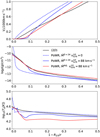 |
Fig. 1 Profile comparison for the O4 star. For visualisation purposes, the 2D averaged model and 1D have been calibrated such that they have the same R2/3. Upper panels : wind velocity profile, in solid black for the 2D spatially averaged model of Debnath et al. (2024), dashed blue for 1D PoWR model with |


3.2 Spectral synthesis
To study the implications of the structures predicted by Debnath et al. (2024) on the spectral diagnosis, we predicted the emergent spectra for all models using the corresponding 1D PoWR models. PoWR calculates the emergent spectrum from a converged 1D model. The radiative transfer is solved in a fixed reference frame (‘observer’s frame’) to obtain the emergent flux and intensity. Electron scattering and line broadening effects are included. Since we only compare model spectra, we do not include any further macroturbulent broadening. Due to the comparably high mass-loss rates – in particular, for the O4 and O2 models – multiple Balmer series members are considerably filled in with wind emission, not only He II 4686 Å. This can blur the effects of the turbulent pressure on the absorption-line wings. We therefore focus our discussion on the Hζ - 3889 Å, He II −4541 Å, and He I −4471 Å spectral lines as shown in Figs. 3, 4, and 5. In red, we show the model approximating the 2D density structure including an adjusted vturb > 0. For comparison, we also show the spectrum of the corresponding model with the same parameters, but removing the turbulent pressure (vturb = 0). It is immediately evident that introducing a vturb > 0 in the hydrostatic equation can have significant consequences on the shape of the spectral lines. In particular, for the wings of the lines, the zero turbulence model shows broader lines than the non-zero solution for the case of Hζ − 3889 Å and He II −4541 Å. The reason is the higher effective surface gravity in the case of zero turbulent pressure (black profiles in Figs. 3 and 4). For the O8 model, the presence of He I −4471 Å in Fig. 5 is highly affected by the turbulence term, while for the earlier types the presence is almost negligible. As the turbulent pressure reduces the effective gravity, one would need to lower the actual surface gravity of the model to mimic the shape of the red profiles if vturb = 0 is assumed (see Section 4.4). The difference in the equivalent width for He I −4471 Å when comparing results from a change in the general He ionisation structure between the two models that is likely induced by the different connection regime resulting from the inclusion of turbulence.
Best-fit final parameters for the 1D PoWR model to match the profile of Debnath et al. (2024).
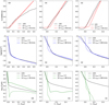 |
Fig. 2 Profile comparison for an O8, O4, and O2 stars. Upper panels: wind velocity profile, in solid black for the 2D spatially averaged model of Debnath et al. (2024), dashed-red for the 1D PoWR model with the best-fit parameters from Table 1 and vturb = 0, and in solid red for the same parameters but vturb > 0, from left to right for the O8, O4, and O2 spectral types, respectively. Middle panels : same as the upper panel, but for the density profile. Lower panel: same as the upper panel, but for the gas temperature. |
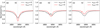 |
Fig. 3 Normalised flux for the HZ line from left to right for the PoWR model spectra calculated for the O8, O4, and O2 models. The red spectrum shows the profile resulting from the model incorporating vturb > 0 to reproduce the 2D average density profile. In black, the spectral lines from a PoWR models with the same parameters, but vturb = 0 is shown. |
4 Discussion
4.1 Turbulence and density profile
We obtained a best-fit result of vturb = 35, 88 and 106 km s−1 for the O8, O4, and O2 stellar models, respectively. We notice that the turbulent velocity increases for earlier spectral types. This effect is a consequence of the closer proximity to the Eddington limit in the earlier models, since the hotter 2D models from Debnath et al. (2024) do not just have different effective temperatures, but also different stellar parameter combinations. As a consequence, the local excess of the Eddington limit at the depth of the iron opacity peak will be higher for earlier- type models, thereby providing the energy and momentum for larger turbulent motion. This is qualitatively aligned with earlier trend predictions from 1D stellar structure calculations for subsurface convection caused by the hot iron-bump (e.g. Cantiello et al. 2009).
In Debnath et al. (2024), the determined mean turbulent velocity is depth-dependent, namely, vturb(r), with a maximum value of ∼80 km s−1 for their O4 model in the sub-photospheric regime. Inwards, vturb gradually decreases to zero in the layers below the iron bump. Outwards, the average turbulent pressure decreases, but the mean turbulent velocity generally increases, albeit not monotonically (cf. Fig. 16 in Debnath et al. 2024).
For our 1D PoWR models, already the assumption of a constant turbulent velocity is sufficient to reproduce the density profile in the outer layers (x = 1 – R2/3/r > 0). The models presented in this work do not cover the regime below the iron opacity peak. Hence, the inner decrease of the turbulent velocity does not need to be covered and a constant value is sufficient (see Section 2.2). However, in the middle panels of Fig. 2, as we go inwards (sub-photosperic layers where x = 1 – R2/3/r < 0) the 1D vturb > 0 profile stars differing from the averaged 2D, challenging our assumption of a constant vturb. Still, assuming a constant vturb already significantly improves our fit and impacts the spectral lines. In future works, we plan to introduce a depth dependence on the turbulence.
4.2 Wind velocity stratification and Mass-loss rate
Figure 1 shows two different radial wind velocity profiles from the 1D models (upper panel): our initial approach, using the same basic stellar parameters as the 2D RHD model, employs a velocity law with β = 0.8, motivated by Pauldrach et al. (1986) as a solid blue line. In the second approach, we increase β > 1 to 1.01 (solid red profile in Fig. 1). Figure2 shows both models with β = 1.01 with and without turbulence. For the wind velocity profile, the effect of the turbulence is to create an onset further out to x ~ 0 (Eq. (5)). Interestingly, this is not the case when comparing to the mass-weighted averages (cf. Fig. B.1), where the onset of the averaged 2D models align much more with the onset we get for the 1D model with turbulence. If we would prescribe the mass-weighted v(r) in a 1D model to infer the density via Eq. (2), we might now in turn expert offsets in the density. As shown in Fig. B.1, the inner part is is problematic due to the complexity going on, but the wind regime looks more promising, although there is indeed a shift for the O8 and O2 model. As we focus on the turbulent (sub-)photospheric structures in this work, we continue our comparison with the non-weighted average.
To improve the fit for the radial velocity in Fig. 2, we have changed the connection settings between the (quasi-)hydrostatic regime and the β–law. Figure D.1 shows the velocity profile modifying the connection point to 0.95 the total local sound speed, instead of the initial 0.95 the effective sound speed accounting for the turbulence. Although the wind velocity profile matches the averaged 2D better, the shift on the connection point negatively affects the agreement with respect to the density around the photosphere.
Each of the spatially averaged 2D wind velocity profiles for the three models (solid-black profiles in the upper panels of Fig. 2) shows a deceleration region (vr < 0) around or just below the photosphere (x ~ 0, Eq. (5)). This reflects that any deeper acceleration of pockets of gas is not sufficient to launch a steady wind, but instead create radiatively-driven turbulent motion and local regions of infalling gas, as reported by Debnath et al. (2024). This non-monotonic behaviour in the (averaged) velocity field cannot be directly mapped in our 1D models, where we connect the hydrostatic solution to a β-law. Testing the spectral imprint of a deceleration region in the photosphere goes beyond the current capabilities of 1D atmosphere models. However, the sub-surface impact of changing the pressure scale height is already accounted for with the introduction of the turbulent pressure term.
In all 2D models, the velocity increase eventually gets more shallow in the outer part, most prominently seen in the O8 model. Since we are assuming a single β–law for the 1D PoWR approach, we cannot reproduce this flattening observed in the 2D models. In principle, a more structured velocity law (e.g. a double-β-law) could be introduced to mitigate this issue. However, this would introduce even more free parameters, which are hard to constrain systematically given the small number of 2D models available.
As reported in Section 3.1, the mass-loss rates of our bestfit 1D models in comparison to the 2D models are increased by 0.1 dex for the O8 model and 0.3 dex for the earlier stellar types. As shown in Fig. 1, this increase in Ṁ is necessary to yield the higher wind density from the 2D average density profile. The mismatch for the model with the same Ṁ could arise from trying to match structures obtained using different methodologies: For example, because of the strong anti-correlation between wind velocity and density in multi-D models (Moens et al. 2022a; Debnath et al. 2024), the average velocity profile ⟨v⟩ will be greater than the density averaged velocity, ⟨ρv⟩/⟨ρ⟩. Therefore, when trying to match a higher ⟨v⟩-structure, a somewhat higher Ṁ will be necessary to obtain the same ⟨ρ⟩. Future investigations of different averages will be needed to see what is best suited to map the structures from a 2D framework in 1D while preserving the averaged parameters as much as possible. Still, the obtained differences in M of a factor of two for the earlier models are not drastic, but would be noticeable in the spectral predictions.
4.3 Electron temperature stratification
While the wind velocity and density profiles can be relatively well reproduced by a PoWR model when compared to the averaged 2D profile (except for the velocity onset of the wind; see discussion in Section 4.2), the temperature stratification shows large differences between both modelling approaches (see the bottom panels in Fig. 2). For all models, the 2D temperature stratification is much smoother than those of the 1D models. The lower panels in Figs. 1 and 2 show the gas temperature stratification for both modelling approaches. The flux temperature calculated from the total emergent flux and the radiation temperature calculated from the integrated mean intensity for the PoWR model is shown in Fig. D.3.
The main difference in the gas temperature profiles between the averaged 2D model and the 1D approach is that while the 2D temperature smoothly decreases, the 1D models present bumps where there is a temperature inversion in the wind regime, for both models with and without turbulence. For the case of the O8 star, there is a moderate temperature increase near the photosphere and the temperature decreases in the outer layers. Compared to the averaged 2D profile, the temperature in the wind region is higher. For the O4 and O2 cases, the temperature inversion occurs at outer layers of the atmosphere. The temperature is also significantly lower than the 2D averaged profile, in particular, for the O2 model. Any inclusion of (micro-)clumping in the 1D models has little effect on the results. Fig. A.1 comparing a smooth with a clumped 1D model reveals that the temperature profile, at least for the given mass-loss rate, is not significantly affected by the change in clumping properties.
These differences in the temperature profiles for both approaches are therefore more likely to arise from differences in the methods used to compute the energy balance in the 1D and 2D models. In the 2D models, the frequency-integrated heating and cooling terms rely on frequency-integrated opacities that have been weighted with the relevant quantities: the energy mean opacity and the Planck mean opacity. In the optically thick static diffusion regime, both the energy and Planck mean opacities, as well as the flux mean opacity present in the radiation force term, are adequately described by the Rosseland mean. However, in the outer wind, where line driving and the Sobolev effect are important (see Sobolev 1960), the Rosseland mean is no longer an accurate approximation. Instead, the three different weighted opacities have to be calculated separately. As mentioned in Section 2.2, methods to get accurate flux-mean opacities have been developed by Poniatowski et al. (2022), but the methods for the energy and Planck mean opacities are still works in progress. Instead, the multi-D models approximate the energy and Planck mean by the flux mean. This very likely results in an over-efficient heating and cooling, which in practice forces the gas and radiation temperatures to the same value, the net effect being a higher gas temperature. This is in contrast to non-LTE models, which typically finds the radiation temperature outside of the photosphere to be higher than the gas temperature. On the other hand, in ID models cooling due to adiabatic expansion in the wind is often neglected and the temperature structure rather obtained from assuming strict radiative equilibrium (or via the equivalent electron thermal balance formalism). It thus remains an open question whether the characteristic temperature inversion often found in ID atmospheric models (see also e.g. discussion in Puls et al. 2005) would survive in multi-D models with a better treatment of the wind energy balance.
Surface gravities, Teff, and masses for vturb > 0, log ɡturb and Mturb/M⊙, and for vturb = 0, log ɡ0, and M0/M⊙ for the three different O star models, as well as the evolutionary mass determined from the HRD position.
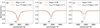 |
Fig. 6 Normalised flux for the Hydrogen Hζ line from left to right for the O8, O4, and O2 stars. Solid-red lines for the best-fit ID PoWR model with vturb > 0, in dashed green for vturb = 0 and lower surface gravity. The stellar parameters for the different models are shown in Table 2. |
4.4 Surface gravity
If the non-zero turbulence (vturb > 0) is included in Eq. (4), it changes the effective pressure scale height in the (quasi-) hydrostatic regime and therefore affects the wings of pressure-broadened absorption lines. Therefore, the fundamental diagnostics for the surface gravity log ɡ are affected such that for vturb > 0, a larger log ɡ value is required to approximately get the same line wings as for vturb = 0. For an assumed constant T(r) ≡ Tphot in the relevant (quasi-)hydrostatic regime, the difference can be estimated as
 (7)
(7)
To illustrate and check this difference in log ɡ, we have decreased the log ɡ for our models with the parameters in Table 1 and without including any turbulence (vturb = 0), denoted as “log ɡ0” in Table 2. The profile comparison for the ‘log ɡ0’ models is shown in Fig. F.1. We compare the spectral lines with the two models in Figs. 6 and 7: in dashed-green lines: the model without any turbulence and decreased log ɡ0 and in solid-red lines: the model with (vturb > 0) and higher log ɡ. We note that for the O2 PoWR model, we could not reach a lower log ɡ0 because of convergence problems, so the results shown in Table 2 for O2 are upper limits. We also take into account the correlation between derived log ɡ and Teff leaving Teff as a free parameter in the models, so that a higher log ɡ requires a higher Teff to keep the He ionisation balance correct.
We estimated the surface gravity difference using Eq. (7), assuming µ ~ 0.6 as of a fully ionised plasma and Tphot = Teff. The difference that we calculate is Δ(log ɡ) = 0.4, 0.9, and 1.0, for the O8, O4, and O2 models, respectively. When compared to log ɡ0 in Table 2, we obtain a Δ(log ɡ) = 0.2, 0.4, and > 0.2 instead. The difference in log ɡ estimated with Eq. (7) differs from the difference when using the values from Table 2 by a factor of two. On the one hand, the differences in fitting the wings of the lines can give rise to a lower Δ(log ɡ0) than predicted by Eq. (7). On the other hand, a secondary effect would be the feedback from the Thomson radiative acceleration for the model without turbulence, Γe,0, as the mass changes but the luminosity remains constant. The ɡturb can be estimated as
 (8)
(8)
where ɡturb is the surface gravity for the model with vturb > 0 and g0 for the model without turbulence, and Γe,0. Using Eq. (8), we find a Δ(log ɡ) = 0.12, 0.75, and 0.81 for the O8, O4, and O2 models, respectively. For the O8 model, the inferred difference from Eq. (8) is 0.08 dex smaller than with the surface gravities from Table 2, providing a closer estimate than with Eq. (7). The large value obtained in Eq. (8) for the O2 model is above the lower limits differences inferred from the surface gravities in Table 2. Eqs. (7) and (8) do not take into account the log ɡ and Teff correlation mentioned earlier, which could explain the difference in the estimated Δ(log ɡ) inferred from the models.
Figures 6 and 7 show the effect of lowering the surface gravity for a model without turbulence as compared to a model with vturb > 0 and higher surface gravity in the spectral lines Hζ − 3889 Å and Hell −4541 Å, where we are able to fit the width of the wings with both the vturb > 0 and log ɡ model and the vturb = 0 and log ɡ0 model. The effect is particularly visible for the O8 and O4 models. While we still cannot perfectly reproduce the width of the wings for the O2 model, due to our results standing as the upper limits, the effects are already visible. Both log ɡ and log ɡ0 models infer two different spectroscopic masses, shown in Table 2 as Mturb /M⊙ and M0 /M⊙ for the model with turbulence and without turbulence, respectively. Figure 8 compares both the vturb > 0 and log ɡ model and the vturb = 0 and log ɡ0 model for He I −4471 Å. In this case, the width of the wings is relatively well reproduced by the 08 model, while the lines are very faint in the 04 and 02 models, but still yield a similar shape for both the vturb > 0 and log ɡ model and the vturb = 0 and log ɡ0 model.
To study the effect on the spectral lines caused by the micro-turbulence broadening term, we have modified ξmin. Fig. E.1 shows the Hζ − 3889 Å line for the 08 model, both for the vturb > 0 and log ɡ model and the lower surface gravity model log ɡ0 and vturb = 0. Moreover, we have included different ξmin in the non-turbulent model to see if we could fit the vturb > 0 line, but we were unable to fit perfectly the depth of the line. Therefore, the influence of ξmin cannot explain the effect on the vturb > 0 for the depth of the lines.
The analysis of O (super-)giants have so far neglected the addition of a turbulence term in the solution of the hydrostatic equation. However, for B supergiants, Weßmayer et al. (2022) performed a quantitative spectroscopic analysis using the ATLAS 12 code (Kurucz 2005), which allows for the inclusion of turbulent pressure. The turbulence was limited to a maximum of 14 km s−1 with resulting Δ(log ɡ) ≈ 0.05 dex. Weßmayer et al. (2022) showed that the addition of a modest turbulence can affect the lines of helium and some metallic lines (Si II, CII and S II).
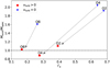 |
Fig. 9 Ratio of Mevol/Mspec with respect to the Thomson radiative acceleration Γe for the models without turbulence (blue triangles) and with turbulence (red squares). We see a shift when we include a turbulent term in the models, obtaining a Mevol/Mspec ratio closer to one. |
4.5 Mass discrepancy
Without the turbulence term but decreased surface gravity, we obtain masses that are ~10 M⊙, ~30 M⊙ and >25 M⊙ lower than when accounting for the turbulence, for the O8, O4, and O2 models, respectively, while the photospheric radius changes by <0.01 R⊙. Noticing the significant change in stellar masses, it is interesting to point out that adding a turbulence term in the hydrostatic equation could therefore potentially solve the so-called ‘mass discrepancy’ problem.
The ‘mass discrepancy’ (e.g. Herrero et al. 1992) for hot stars refers to a difference between stellar mass estimations from evolutionary tracks and the positions of the stars in the Hertzsprung-Russell diagram (‘evolutionary masses’) and the spectroscopically derived masses. Typically, the evolutionary masses are higher than the spectroscopic masses. In the original report of the problem by Herrero et al. (1992), stars closer to the Eddington limit showed a stronger discrepancy, which would align very well with the obtained turbulence trend. Comparing the luminosities and effective temperatures of our models (see Table 1) with the stellar evolution tracks from Ekström et al. (2012), we estimated the corresponding evolutionary masses, Mevol/M⊙ (see Appendix G for details), shown in Table 2. Figure 9 shows the Mevol/Mspec ratio with respect to the Thomson radiative acceleration, Γe, for the models with vturb > 0 (red squares) and the models with vturb = 0 and log g0 (blue triangles). We see a clear shift when we include a turbulent term in the models, obtaining a Mevol/Mspec ratio closer to one, thereby reconciling both mass determinations.
When comparing to spectroscopic data, Markova et al. (2018) analysed optical spectra of 53 Galactic O stars using the FAST-WIND and CMFGEN codes and compared to published predictions of evolutionary model grids by Brott et al. (2011) and Ekström et al. (2012). We checked an example star, HD 46223 from Markova et al. (2018), with the spectral type 04 V and comparable stellar parameters to our O4 model, such as the effective temperature (Teff = 43.5 ± 1.5 kK), surface gravity (log ɡ = 3.95 ± 0.1), stellar radius (R★ = 10.9 ± 2.0 R⊙), and luminosity (log(L★/L⊙) = 5.58 ± 0.17); whereas those authors obtained a spectroscopic mass (Mspec = 38.9 ± 14.4M⊙), which is ~20 M⊙ lower than our estimated stellar mass for the 04 model, including the turbulence term. For the case of HD 46223 in Markova et al. (2018), all the evolutionary track predictions overestimate the mass by at least 8 M⊙, obtaining a Mevol value comparable to ours when including the turbulence (Mevol = 47.0 – 51.8 M⊙, depending on the evolutionary track used). In this particular example, we find that one systematically underestimates the spectroscopic mass and so, accounting for the turbulent pressure in the hydrostatic equation could potentially reconcile both mass measurements. However, we notice that the log ɡ for HD 46223 is significantly higher than that of our 04 model. Therefore, there is a need for more spectroscopic studies to include a wider range of spectral types, along with a turbulence term to determine the regime where the mass discrepancy could be reconciled.
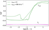 |
Fig. 10 Radiative acceleration (total and Thomson) normalised to gravity as a function of radius for two ID models resembling the 04 2D average. The two models only differ in their turbulent pressure which is included in the (quasi-)hydrostatic domain. |
4.6 Influence on the radiative force
In the 1D PoWR models, the inclusion of turbulent pressure in the (quasi-)hydrostatic regime also has a profound impact in the resulting radiative acceleration of the converged stationary models. In Fig. 10, we plot the radiative acceleration normalised to gravity (Γrad) for our ID models with and without turbulent pressure approximating the 2D-average from the O4 model by Debnath et al. (2024). The characteristic ‘dip’ in the radiative acceleration, which typically occurs just before the onset of the wind (see, e.g. Sander et al. 2015; Sundqvist et al. 2019), is only prominent in the model without turbulent pressure, while the model including turbulence has a much smoother (albeit lower) radiative acceleration in the hydrostatic regime. For comparison, we further show the radiative acceleration for the 08 and 02 ID models in Appendix H. Similarly to the 04 model, the ‘dip’ in the O2 case is smoothed out when introducing a vturb term. This is not the case for the O8 model, where the ‘dip’ is changed, but remains prominent. The reason is the more modest value of vturb = 35 km s−1 in comparison with the earlier O-types, which seems to be insufficient with respect to avoiding the formation of a pronounced ‘dip’.
Our ID models in this work are not hydrodynamically consistent, therefore, they cannot predict mass-loss rates intrinsically. Nonetheless, they are sufficient to allow us to conclude that the inclusion of a turbulent pressure could have significant consequences on mass-loss predictions, due to the resulting change of the Γrad-slope. The lower average of Γrad in the (quasi-)hydrostatic regime could give rise to the assumption that resulting mass-loss rates from ID dynamical calculations might be even lower. On the other hand, the avoidance of the ‘dip’ is expected to change the iteration process and might help avoid a drop to much lower values, at least in regimes where considerable turbulent velocity is expected and provides an additional outward-directed force. With the presumed trend towards higher turbulence for earlier spectral types, consequences are expected to be larger for hotter and more massive stars. None of this has been covered thus far in any of the existing theoretical mass-loss prescriptions for OB stars (e.g. Vink et al. 2001; Krtička & Kubát 2018; Björklund et al. 2023), with the resulting effects likely being very regime-specific, potentially leading to stronger differences between supergiants (which are closer to the Edding-ton limit) and dwarfs. On the other hand, the average mass-loss rates computed from the three 2D O-star simulations investigated here are fairly well-aligned with the predictions by Krtička & Kubát (2018); Björklund et al. (2023) (see Fig. 18 in Debnath et al. 2024). This is indeed surprising given the lack of turbulent pressure in the ID models underlying these Ṁ predictions. New, dynamically consistent, ID calculations will be necessary to investigate this further, however, this is beyond the scope of the present exploratory paper.
5 Conclusions
We calculated 1D stellar atmosphere models with the PoWR code to resemble the averaged 2D profiles of three O-star RHD simulations from Debnath et al. (2024). The average density profiles can be aptly reproduced by including a turbulent velocity term in the solution of the hydrostatic equation of motion. While Debnath et al. (2024) reported a depth-dependency for their inferred turbulent velocity, we find that a constant turbulent velocity is sufficient to reproduce the relevant part of the mean 2D density profile in our ID models reasonably well. This simplification is possible due to the fact that in the 2D models, there is a large increase of the averaged turbulence that takes place in the optically thick deeper layers, which does not influence the spectrum. In the future, we plan to include a depth-dependent turbulence to test variations of the turbulent velocity, its predicted increase in the supersonic regime, and the potential impact on the inferred wind driving.
In our attempt to reproduce the wind velocity profile, we employed a β = 1.01–law for the supersonic part of the model. While this differs from the most-common value for O-stars of β = 0.8 (e.g. Pauldrach et al. 1986), increasing β improves the connection to the (quasi-)hydrostatic part and shifts the increase in the velocity outwards, thereby producing a similar slope to the profiles from Debnath et al. (2024). A closer connection point between the hydrostatic and the β-law domain shifts the increase of the velocity inwards, thereby improving the agreement with the 2D-averaged velocity field; however, at the same time, this worsens the fit of the 2D-averaged density distribution in the transition regime. Thus, it remains a challenge to find suitable velocity laws for this important transition region in unified model atmospheres connecting a quasi-hydrostatic photosphere to an outflowing wind, described by an analytic β-law. Considering weighted averages, such as the mass-weighted average, might help to reconcile discrepancies in the wind-onset and outer wind region. Ideally, this should be investigated jointly with observations and diagnostics sensitive to this region, which is beyond the present prototype study.
The addition of a turbulent pressure also has an impact on the derived radiative acceleration in the (quasi-)hydrostatic domain of the 1D PoWR models. When a significant turbulent motion is added in the solution of the hydrostatic equation, the acceleration slope becomes smoother and typical ‘dip-like’ structures can be avoided. With its effect on the radiative acceleration profile, the inclusion of turbulent pressure will most likely also affect future mass-loss rate predictions from 1D hydrodynamically-consistent model atmospheres.
The change in the scale height by the introduction of a non-negligible turbulent pressure term affects the resulting spectral line diagnostics, yielding higher values for log ɡ and Mspec, compared to similar models that do not include turbulence. Therefore, including this extra turbulent pressure could diminish or in some cases even remove the so-called ‘mass discrepancy’ between the inferred evolutionary and spectroscopic masses. Ultimately, our findings underline the need for a better treatment of the outer layers in evolutionary models to enable more coherent comparisons with spectroscopic results. While we only discuss three sets of models in this work, a broader investigation of the O and B star regime with both multi-D and 1D models will be necessary to infer proper associations of vturb with spectral types, macroturbulence, or other parameter correlations necessary to systematically account for turbulent pressure in the spectral analysis of massive stars.
Acknowledgements
GGT is supported by the German Deutsche Forschungs-gemeinschaft (DFG) under Project-ID 496854903 (SA4064/2-1, PI Sander). AACS, RRL, and JJ are supported by the German Deutsche Forschungsge-meinschaft (DFG) under Project-ID 445674056 (Emmy Noether Research Group SA4064/1-1, PI Sander). GGT and AACS further acknowledge support from the Federal Ministry of Education and Research (BMBF) and the Baden-Württemberg Ministry of Science as part of the Excellence Strategy of the German Federal and State Governments. JOS, DD, LD, NM, CVdS acknowledge the support of the European Research Council (ERC) Horizon Europe grant under grant agreement number 101044048 (ERC-2021-COG, SUPERSTARS-3D). OV, JOS, and LD acknowledge the support of the Belgian Research Foundation Flanders (FWO) Odysseus program under grant number G0H9218N and FWO grant G077822N.
Appendix A O4 smooth model
 |
Fig. A.1 Profile comparison for a smooth 04 model (dashed-blue) and a model with density contrast D = 10 (solid-red). Right panels: Wind velocity profile. Middle panel: Same as the left panel, but for the density profile. Left panel: Same as the left panel, but for the gas temperature. |
 |
Fig. A.2 Spectral line comparison for a smooth O4 model (dashed-blue) and a model with density contrast D = 10 (solid-red) in the optical. The rest of the parameters for both models are the same. |
Appendix B Mass-weighted velocity profile
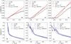 |
Fig. B.1 Mass-weighted averaged 2D profiles. Upper panels: Mass-weighted averaged 2D velocity ( |

Appendix C Profile comparison with respect to τRoss
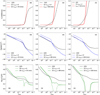 |
Fig. C.1 Profile comparison for an O8, O4 and O2 stars with respect to the Rosseland mean opacity, τRoss. Upper panels: Wind velocity profile, in solid black for the 2D averaged model of Debnath et al. (2024), dashed-red for the ID PoWR model with the best-fit parameters from Table 1 and vturb = 0, and in solid red for the same parameters but vturb > 0, from left to right for the 08, 04 and 02 spectral types, respectively. Middle panels: Same as the upper panel, but for the density profile. Lower panel: Same as the upper panel, but for the gas temperature. |
Appendix D Connection point, velocity gradient, and radiative temperature
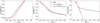 |
Fig. D.1 Profile comparison for the O2 model shifting the connection point between the (quasi-)hydrostatic regime and the β–law. Left panel: Wind velocity profile, in solid black for the 2D averaged model of Debnath et al. (2024), solid red for the best-fit 1D PoWR model with vturb > 0 and initial connection point (vturb = 0.95 vsonicturb), in dotted blue for the shifted connection point (vcon = 0.95 vsonic). Middle panel: Same as the left panel, but for the density profile. Right panel: Same as the left panel, but for the gas temperature. |
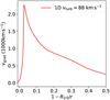 |
Fig. D.2 Velocity gradient for the 04 model with vturb > 0. We can distinguish two different regimes: the hydrostatic regiome with x ≤ 0.1 and the β-law regime with x > 0.1 |
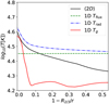 |
Fig. D.3 Flux temperature (dashed green line) and radiation temperature (dashed blue line) for the 04 model with vturb > 0 obtained from the total emergent flux, compared to the gas temperature stratifications for the averaged 〈2D〉 and the 1D vturb > 0 models. |
Appendix E ξ broadening effect in the spectral synthesis
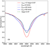 |
Fig. E.1 Influence on the ξmin microturbulence broadening term in the spectral synthesis for the Hζ line. In red the 1D fit with vturb > 0, in dash-dotted green the model with vturb = 0 and a lower log ɡ with standard ξ = 10 km s−1, in blue the models with vturb = 0 and a lower log ɡ changing the ξmin with 0, 20 and 50 km s−1. The influence of ξmin does not explain the effect on the vturb > 0 for the depth of the lines. |
Appendix F Profile comparison for log ɡ0
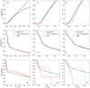 |
Fig. F.1 Profile comparison for an O8, O4, and O2 stars. Upper panels: Wind velocity profile, in solid black for the 2D averaged model of Debnath et al. (2024), solid red for the best-fit 1D PoWR model with vturb > 0, in dashed green for vturb = 0 and lower surface gravity, from left to right for the O8, O4, O2 spectral types, respectively. Middle panels: Same as the upper panel, but for the density profile. Lower panel: Same as the upper panel, but for the gas temperature. |
Appendix G Determination of evolutionary masses
To determine the evolutionary masses of our models, we plotted their position in the HRD alongside the GENEC tracks at Galactic metallicity by Ekström et al. (2012), as shown in Fig G.1. We performed a linear interpolation of the tracks in log(Mini) and selected the best-fitting tracks by eye to the nearest 0.5M⊙ in initial mass. We then extract the current mass of the interpolated track at the point that lies closest to our data points in the HRD. The evolutionary masses obtained this way have an estimated error margin of ±0.5M⊙ (without accounting for systematic errors in the evolution code) and are presented alongside the masses obtained in the atmosphere fitting in Table 2.
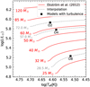 |
Fig. G.1 Hertzsprung-Russell diagram showing our models against the stellar evolution tracks of Ekström et al. (2012) with the best-fit interpolated tracks. |
Appendix H Radiative acceleration
References
- Aschenbrenner, P., Przybilla, N., & Butler, K. 2023, A&A, 671, A36 [NASA ADS] [CrossRef] [EDP Sciences] [Google Scholar]
- Asplund, M., Grevesse, N., Sauval, A. J., & Scott, P. 2009, ARA&A, 47, 481 [NASA ADS] [CrossRef] [Google Scholar]
- Björklund, R., Sundqvist, J. O., Singh, S. M., Puls, J., & Najarro, F. 2023, A&A, 676, A109 [NASA ADS] [CrossRef] [EDP Sciences] [Google Scholar]
- Bouret, J. C., Lanz, T., Hillier, D. J., et al. 2003, ApJ, 595, 1182 [NASA ADS] [CrossRef] [Google Scholar]
- Bouret, J. C., Hillier, D. J., Lanz, T., & Fullerton, A. W. 2012, A&A, 544, A67 [NASA ADS] [CrossRef] [EDP Sciences] [Google Scholar]
- Brott, I., de Mink, S. E., Cantiello, M., et al. 2011, A&A, 530, A115 [NASA ADS] [CrossRef] [EDP Sciences] [Google Scholar]
- Cantiello, M., Langer, N., Brott, I., et al. 2009, A&A, 499, 279 [NASA ADS] [CrossRef] [EDP Sciences] [Google Scholar]
- Carneiro, L. P., Puls, J., Hoffmann, T. L., Holgado, G., & Simón-Díaz, S. 2019, A&A, 623, A3 [NASA ADS] [CrossRef] [EDP Sciences] [Google Scholar]
- Castor, J. I., Abbott, D. C., & Klein, R. I. 1975, ApJ, 195, 157 [Google Scholar]
- Debnath, D., Sundqvist, J. O., Moens, N., et al. 2024, A&A, 684, A177 [NASA ADS] [CrossRef] [EDP Sciences] [Google Scholar]
- Dessart, L., & Owocki, S. P. 2005, A&A, 437, 657 [NASA ADS] [CrossRef] [EDP Sciences] [Google Scholar]
- Ekström, S., Georgy, C., Eggenberger, P., et al. 2012, A&A, 537, A146 [Google Scholar]
- Gayley, K. G. 1995, ApJ, 454, 410 [Google Scholar]
- Gräfener, G., Koesterke, L., & Hamann, W. R. 2002, A&A, 387, 244 [NASA ADS] [CrossRef] [EDP Sciences] [Google Scholar]
- Grevesse, N., & Noels, A. 1993, in Origin and Evolution of the Elements, eds. N. Prantzos, E. Vangioni-Flam, & M. Casse, 15 [Google Scholar]
- Hainich, R., Ramachandran, V., Shenar, T., et al. 2019, A&A, 621, A85 [NASA ADS] [CrossRef] [EDP Sciences] [Google Scholar]
- Hainich, R., Oskinova, L. M., Torrejón, J. M., et al. 2020, A&A, 634, A49 [NASA ADS] [CrossRef] [EDP Sciences] [Google Scholar]
- Hamann, W. R. 1986, A&A, 160, 347 [NASA ADS] [Google Scholar]
- Hamann, W. R., & Gräfener, G. 2003, A&A, 410, 993 [CrossRef] [EDP Sciences] [Google Scholar]
- Hawcroft, C., Sana, H., Mahy, L., et al. 2021, A&A, 655, A67 [NASA ADS] [CrossRef] [EDP Sciences] [Google Scholar]
- Hennicker, L., Puls, J., Kee, N. D., & Sundqvist, J. O. 2018, A&A, 616, A140 [NASA ADS] [CrossRef] [EDP Sciences] [Google Scholar]
- Herrero, A., Kudritzki, R. P., Vilchez, J. M., et al. 1992, A&A, 261, 209 [NASA ADS] [Google Scholar]
- Hillier, D. J. 2003, in Astronomical Society of the Pacific Conference Series, 288, Stellar Atmosphere Modeling, eds. I. Hubeny, D. Mihalas, & K. Werner, 199 [NASA ADS] [Google Scholar]
- Hillier, D. J., & Miller, D. L. 1998, ApJ, 496, 407 [NASA ADS] [CrossRef] [Google Scholar]
- Hillier, D. J., Lanz, T., Heap, S. R., et al. 2003, ApJ, 588, 1039 [Google Scholar]
- Howarth, I. D., Siebert, K. W., Hussain, G. A. J., & Prinja, R. K. 1997, MNRAS, 284, 265 [NASA ADS] [CrossRef] [Google Scholar]
- Hubeny, I., & Lanz, T. 2003, in Astronomical Society of the Pacific Conference Series, 288, Stellar Atmosphere Modeling, eds. I. Hubeny, D. Mihalas, & K. Werner, 51 [NASA ADS] [Google Scholar]
- Iglesias, C. A., & Rogers, F. J. 1996, ApJ, 464, 943 [NASA ADS] [CrossRef] [Google Scholar]
- Jiang, Y.-F., Cantiello, M., Bildsten, L., Quataert, E., & Blaes, O. 2015, ApJ, 813, 74 [Google Scholar]
- Koesterke, L., Hamann, W. R., & Gräfener, G. 2002, A&A, 384, 562 [NASA ADS] [CrossRef] [EDP Sciences] [Google Scholar]
- Krtička, J., & Kubát, J. 2018, A&A, 612, A20 [NASA ADS] [CrossRef] [EDP Sciences] [Google Scholar]
- Kubát, J., Puls, J., & Pauldrach, A. W. A. 1999, A&A, 341, 587 [NASA ADS] [Google Scholar]
- Kurucz, R. L. 2005, Mem. Soc. Astron. Ital. Suppl., 8, 14 [Google Scholar]
- Lefever, R. R., Sander, A. A. C., Shenar, T., et al. 2023, MNRAS, 521, 1374 [NASA ADS] [CrossRef] [Google Scholar]
- Marcolino, W. L. F., Bouret, J. C., Martins, F., et al. 2009, A&A, 498, 837 [NASA ADS] [CrossRef] [EDP Sciences] [Google Scholar]
- Markova, N., Puls, J., & Langer, N. 2018, A&A, 613, A12 [NASA ADS] [CrossRef] [EDP Sciences] [Google Scholar]
- Moens, N., Poniatowski, L. G., Hennicker, L., et al. 2022a, A&A, 665, A42 [NASA ADS] [CrossRef] [EDP Sciences] [Google Scholar]
- Moens, N., Sundqvist, J. O., El Mellah, I., et al. 2022b, A&A, 657, A81 [NASA ADS] [CrossRef] [EDP Sciences] [Google Scholar]
- Najarro, F., Hanson, M. M., & Puls, J. 2011, A&A, 535, A32 [NASA ADS] [CrossRef] [EDP Sciences] [Google Scholar]
- Owocki, S. P., & Puls, J. 1999, ApJ, 510, 355 [Google Scholar]
- Pauldrach, A., Puls, J., & Kudritzki, R. P. 1986, A&A, 164, 86 [NASA ADS] [Google Scholar]
- Pomraning, G. C. 1988, J. Quant. Spec. Radiat. Transf., 40, 479 [NASA ADS] [CrossRef] [Google Scholar]
- Poniatowski, L. G., Kee, N. D., Sundqvist, J. O., et al. 2022, A&A, 667, A113 [NASA ADS] [CrossRef] [EDP Sciences] [Google Scholar]
- Portinari, L., Chiosi, C., & Bressan, A. 1998, A&A, 334, 505 [NASA ADS] [Google Scholar]
- Puls, J. 2008, in Massive Stars as Cosmic Engines, 250, eds. F. Bresolin, P. A. Crowther, & J. Puls, 25 [NASA ADS] [Google Scholar]
- Puls, J., Urbaneja, M. A., Venero, R., et al. 2005, A&A, 435, 669 [NASA ADS] [CrossRef] [EDP Sciences] [Google Scholar]
- Ramachandran, V., Hainich, R., Hamann, W. R., et al. 2018, A&A, 609, A7 [NASA ADS] [CrossRef] [EDP Sciences] [Google Scholar]
- Ramírez-Agudelo, O. H., Sana, H., de Koter, A., et al. 2017, A&A, 600, A81 [NASA ADS] [CrossRef] [EDP Sciences] [Google Scholar]
- Rübke, K., Herrero, A., & Puls, J. 2023, A&A, 679, A19 [NASA ADS] [CrossRef] [EDP Sciences] [Google Scholar]
- Sabhahit, G. N., Vink, J. S., Sander, A. A. C., & Higgins, E. R. 2023, MNRAS, 524, 1529 [NASA ADS] [CrossRef] [Google Scholar]
- Sander, A. A. C. 2015, PhD thesis, University of Potsdam, Germany [Google Scholar]
- Sander, A. A. C. 2017, in The Lives and Death-Throes of Massive Stars, 329, eds. J. J. Eldridge, J. C. Bray, L. A. S. McClelland, & L. Xiao, 215 [NASA ADS] [Google Scholar]
- Sander, A. A. C., & Vink, J. S. 2020, MNRAS, 499, 873 [Google Scholar]
- Sander, A., Shenar, T., Hainich, R., et al. 2015, A&A, 577, A13 [NASA ADS] [CrossRef] [EDP Sciences] [Google Scholar]
- Sander, A. A. C., Hamann, W. R., Todt, H., Hainich, R., & Shenar, T. 2017, A&A, 603, A86 [NASA ADS] [CrossRef] [EDP Sciences] [Google Scholar]
- Sander, A. A. C., Vink, J. S., & Hamann, W. R. 2020, MNRAS, 491, 4406 [Google Scholar]
- Sander, A. A. C., Lefever, R. R., Poniatowski, L. G., et al. 2023, A&A, 670, A83 [NASA ADS] [CrossRef] [EDP Sciences] [Google Scholar]
- Sander, A. A. C., Bouret, J. C., Bernini-Peron, M., et al. 2024, A&A, 689, A30 [NASA ADS] [CrossRef] [EDP Sciences] [Google Scholar]
- Schultz, W. C., Bildsten, L., & Jiang, Y.-F. 2022, ApJ, 924, L11 [NASA ADS] [CrossRef] [Google Scholar]
- Shenar, T., Oskinova, L., Hamann, W. R., et al. 2015, ApJ, 809, 135 [Google Scholar]
- Simón-Díaz, S., Godart, M., Castro, N., et al. 2017, A&A, 597, A22 [CrossRef] [EDP Sciences] [Google Scholar]
- Sobolev, V. V. 1960, Moving Envelopes of Stars [Google Scholar]
- Sundqvist, J. O., Puls, J., & Feldmeier, A. 2010, A&A, 510, A11 [NASA ADS] [CrossRef] [EDP Sciences] [Google Scholar]
- Sundqvist, J. O., Owocki, S. P., & Puls, J. 2018, A&A, 611, A17 [NASA ADS] [CrossRef] [EDP Sciences] [Google Scholar]
- Sundqvist, J. O., Björklund, R., Puls, J., & Najarro, F. 2019, A&A, 632, A126 [NASA ADS] [CrossRef] [EDP Sciences] [Google Scholar]
- Šurlan, B., Hamann, W. R., Kubát, J., Oskinova, L. M., & Feldmeier, A. 2012, A&A, 541, A37 [NASA ADS] [CrossRef] [EDP Sciences] [Google Scholar]
- Verhamme, O., Sundqvist, J., de Koter, A., et al. 2024, A&A, 692, A91 [NASA ADS] [CrossRef] [EDP Sciences] [Google Scholar]
- Vink, J. S., de Koter, A., & Lamers, H. J. G. L. M. 2001, A&A, 369, 574 [NASA ADS] [CrossRef] [EDP Sciences] [Google Scholar]
- Vink, J. S., Mehner, A., Crowther, P. A., et al. 2023, A&A, 675, A154 [NASA ADS] [CrossRef] [EDP Sciences] [Google Scholar]
- Weßmayer, D., Przybilla, N., & Butler, K. 2022, A&A, 668, A92 [NASA ADS] [CrossRef] [EDP Sciences] [Google Scholar]
- Xia, C., Teunissen, J., El Mellah, I., Chané, E., & Keppens, R. 2018, ApJS, 234, 30 [Google Scholar]
All Tables
Best-fit final parameters for the 1D PoWR model to match the profile of Debnath et al. (2024).
Surface gravities, Teff, and masses for vturb > 0, log ɡturb and Mturb/M⊙, and for vturb = 0, log ɡ0, and M0/M⊙ for the three different O star models, as well as the evolutionary mass determined from the HRD position.
All Figures
|
Fig. 1 Profile comparison for the O4 star. For visualisation purposes, the 2D averaged model and 1D have been calibrated such that they have the same R2/3. Upper panels : wind velocity profile, in solid black for the 2D spatially averaged model of Debnath et al. (2024), dashed blue for 1D PoWR model with |
| In the text | |
|
Fig. 2 Profile comparison for an O8, O4, and O2 stars. Upper panels: wind velocity profile, in solid black for the 2D spatially averaged model of Debnath et al. (2024), dashed-red for the 1D PoWR model with the best-fit parameters from Table 1 and vturb = 0, and in solid red for the same parameters but vturb > 0, from left to right for the O8, O4, and O2 spectral types, respectively. Middle panels : same as the upper panel, but for the density profile. Lower panel: same as the upper panel, but for the gas temperature. |
| In the text | |
|
Fig. 3 Normalised flux for the HZ line from left to right for the PoWR model spectra calculated for the O8, O4, and O2 models. The red spectrum shows the profile resulting from the model incorporating vturb > 0 to reproduce the 2D average density profile. In black, the spectral lines from a PoWR models with the same parameters, but vturb = 0 is shown. |
| In the text | |
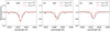 |
Fig. 4 Same as Figure 3, but for the He II −4541 Å line. |
| In the text | |
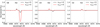 |
Fig. 5 Same as Figure 3, but for the He I −4471 Å line. |
| In the text | |
|
Fig. 6 Normalised flux for the Hydrogen Hζ line from left to right for the O8, O4, and O2 stars. Solid-red lines for the best-fit ID PoWR model with vturb > 0, in dashed green for vturb = 0 and lower surface gravity. The stellar parameters for the different models are shown in Table 2. |
| In the text | |
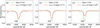 |
Fig. 7 Same as Figure 6, but for the HeII line. |
| In the text | |
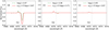 |
Fig. 8 Same as Figure 6, but for the HeI line. |
| In the text | |
|
Fig. 9 Ratio of Mevol/Mspec with respect to the Thomson radiative acceleration Γe for the models without turbulence (blue triangles) and with turbulence (red squares). We see a shift when we include a turbulent term in the models, obtaining a Mevol/Mspec ratio closer to one. |
| In the text | |
|
Fig. 10 Radiative acceleration (total and Thomson) normalised to gravity as a function of radius for two ID models resembling the 04 2D average. The two models only differ in their turbulent pressure which is included in the (quasi-)hydrostatic domain. |
| In the text | |
|
Fig. A.1 Profile comparison for a smooth 04 model (dashed-blue) and a model with density contrast D = 10 (solid-red). Right panels: Wind velocity profile. Middle panel: Same as the left panel, but for the density profile. Left panel: Same as the left panel, but for the gas temperature. |
| In the text | |
|
Fig. A.2 Spectral line comparison for a smooth O4 model (dashed-blue) and a model with density contrast D = 10 (solid-red) in the optical. The rest of the parameters for both models are the same. |
| In the text | |
|
Fig. B.1 Mass-weighted averaged 2D profiles. Upper panels: Mass-weighted averaged 2D velocity ( |
| In the text | |
|
Fig. C.1 Profile comparison for an O8, O4 and O2 stars with respect to the Rosseland mean opacity, τRoss. Upper panels: Wind velocity profile, in solid black for the 2D averaged model of Debnath et al. (2024), dashed-red for the ID PoWR model with the best-fit parameters from Table 1 and vturb = 0, and in solid red for the same parameters but vturb > 0, from left to right for the 08, 04 and 02 spectral types, respectively. Middle panels: Same as the upper panel, but for the density profile. Lower panel: Same as the upper panel, but for the gas temperature. |
| In the text | |
|
Fig. D.1 Profile comparison for the O2 model shifting the connection point between the (quasi-)hydrostatic regime and the β–law. Left panel: Wind velocity profile, in solid black for the 2D averaged model of Debnath et al. (2024), solid red for the best-fit 1D PoWR model with vturb > 0 and initial connection point (vturb = 0.95 vsonicturb), in dotted blue for the shifted connection point (vcon = 0.95 vsonic). Middle panel: Same as the left panel, but for the density profile. Right panel: Same as the left panel, but for the gas temperature. |
| In the text | |
|
Fig. D.2 Velocity gradient for the 04 model with vturb > 0. We can distinguish two different regimes: the hydrostatic regiome with x ≤ 0.1 and the β-law regime with x > 0.1 |
| In the text | |
|
Fig. D.3 Flux temperature (dashed green line) and radiation temperature (dashed blue line) for the 04 model with vturb > 0 obtained from the total emergent flux, compared to the gas temperature stratifications for the averaged 〈2D〉 and the 1D vturb > 0 models. |
| In the text | |
|
Fig. E.1 Influence on the ξmin microturbulence broadening term in the spectral synthesis for the Hζ line. In red the 1D fit with vturb > 0, in dash-dotted green the model with vturb = 0 and a lower log ɡ with standard ξ = 10 km s−1, in blue the models with vturb = 0 and a lower log ɡ changing the ξmin with 0, 20 and 50 km s−1. The influence of ξmin does not explain the effect on the vturb > 0 for the depth of the lines. |
| In the text | |
|
Fig. F.1 Profile comparison for an O8, O4, and O2 stars. Upper panels: Wind velocity profile, in solid black for the 2D averaged model of Debnath et al. (2024), solid red for the best-fit 1D PoWR model with vturb > 0, in dashed green for vturb = 0 and lower surface gravity, from left to right for the O8, O4, O2 spectral types, respectively. Middle panels: Same as the upper panel, but for the density profile. Lower panel: Same as the upper panel, but for the gas temperature. |
| In the text | |
|
Fig. G.1 Hertzsprung-Russell diagram showing our models against the stellar evolution tracks of Ekström et al. (2012) with the best-fit interpolated tracks. |
| In the text | |
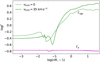 |
Fig. H.1 Same as Figure 10, but for the O8 model. |
| In the text | |
 |
Fig. H.2 Same as Figure 10, but for the O2 model. |
| In the text | |
Current usage metrics show cumulative count of Article Views (full-text article views including HTML views, PDF and ePub downloads, according to the available data) and Abstracts Views on Vision4Press platform.
Data correspond to usage on the plateform after 2015. The current usage metrics is available 48-96 hours after online publication and is updated daily on week days.
Initial download of the metrics may take a while.